Massive Lossless Data Compression and Multiple Parameter Estimation from Galaxy Spectra
Abstract
We present a method for radical linear compression of datasets where the data are dependent on some number of parameters. We show that, if the noise in the data is independent of the parameters, we can form linear combinations of the data which contain as much information about all the parameters as the entire dataset, in the sense that the Fisher information matrices are identical; i.e. the method is lossless. We explore how these compressed numbers fare when the noise is dependent on the parameters, and show that the method, although not precisely lossless, increases errors by a very modest factor. The method is general, but we illustrate it with a problem for which it is well-suited: galaxy spectra, whose data typically consist of fluxes, and whose properties are set by a handful of parameters such as age, brightness and a parametrised star formation history. The spectra are reduced to a small number of data, which are connected to the physical processes entering the problem. This data compression offers the possibility of a large increase in the speed of determining physical parameters. This is an important consideration as datasets of galaxy spectra reach in size, and the complexity of model spectra increases. In addition to this practical advantage, the compressed data may offer a classification scheme for galaxy spectra which is based rather directly on physical processes.
1 Introduction
There are many instances where objects consist of many data, whose values are determined by a small number of parameters. Often, it is only these parameters which are of interest. The aim of this paper is to find linear combinations of the data which are focussed on estimating the physical parameters with as small an error as possible. Such a problem is very general, and has been attacked in the case of parameter estimation in large-scale structure and the microwave background (e.g. ? [hereafter TTH], ?, ?, ?). Previous work has concentrated largely on the estimation of a single parameter; the main advance of this paper is that it sets out a method for the estimation of multiple parameters. The method provides one projection per parameter, with the consequent possibility of a massive data compression factor. Furthermore, if the noise in the data is independent of the parameters, then the method is entirely lossless. i.e. the compressed dataset contains as much information about the parameters as the full dataset, in the sense that the Fisher information matrix is the same for the compressed dataset as the entire original dataset. An equivalent statement is that the mean likelihood surface is at the peak locally identical when the full or compressed data are used.
We illustrate the method with the case of galaxy spectra, for which there are surveys underway which will provide objects. In this application, the noise is generally not independent of the parameters, as there is a photon shot-noise component which depends on how many photons are expected. We take a spectrum with poor signal-to-noise, whose noise is approximately from photon counting alone, and investigate how the method fares. In this case, the method is not lossless, but the increase in error bars is shown to be minimal, and superior in this respect to an alternative compression system PCA (Principal Component Analysis).
One advantage such radical compression offers is speed of analysis. One major scientific goal of galaxy spectral surveys is to determine physical parameters of the stellar component of the galaxies, such as the age, star formation history, initial mass function and so on. Such a process can, in principle, be achieved by generating model galaxy spectra by stellar population synthesis techniques, and finding the best-fitting model by maximum-likelihood techniques. This can be very time-consuming, and must inevitably be automated for so many galaxies. In addition, one may have a large parameter space to explore, so any method which can speed up this process is worth investigation. One possible further application of the data compression method is that the handful of numbers might provide the basis of a classification scheme which is based on the physical properties one wants to measure.
The outline of the paper is as follows: in section II we set out the lossless compression method for noise which is independent of the parameters; the proof appears in the appendix. In section III we discuss the more general case where the noise covariance matrix and the mean signal both depend on the parameters. In section IV we show through a worked example of galaxy spectra that the method, although not lossless, works very well in the general case.
2 Method
We represent our data by a vector , (e.g. a set of fluxes at different wavelengths). These measurements include a signal part, which we denote by , and noise, :
| (1) |
Assuming the noise has zero mean, . The signal will depend on a set of parameters , which we wish to determine. For galaxy spectra, the parameters may be, for example, age, magnitude of source, metallicity and some parameters describing the star formation history. Thus, is a noise-free spectrum of a galaxy with certain age, metallicity etc.
The noise properties are described by the noise covariance matrix, , with components . If the noise is gaussian, the statistical properties of the data are determined entirely by and . In principle, the noise can also depend on the parameters. For example, in galaxy spectra, one component of the noise will come from photon counting statistics, and the contribution of this to the noise will depend on the mean number of photons expected from the source.
The aim is to derive the parameters from the data. If we assume uniform priors for the parameters, then the a posteriori probability for the parameters is the likelihood, which for gaussian noise is
| (2) | |||||
One approach is simply to find the (highest) peak in the likelihood, by exploring all parameter space, and using all pixels. The position of the peak gives estimates of the parameters which are asymptotically (low noise) the best unbiased estimators (see TTH). This is therefore the best we can do. The maximum-likelihood procedure can, however, be time-consuming if is large, and the parameter space is large. The aim of this paper is to see whether we can reduce the numbers to a smaller number, without increasing the uncertainties on the derived parameters . To be specific, we try to find a number of linear combinations of the spectral data x which encompass as much as possible of the information about the physical parameters. We find that this can be done losslessly in some circumstances; the spectra can be reduced to a handful of numbers without loss of information. The speed-up in parameter estimation is about a factor .
In general, reducing the dataset in this way will lead to larger error bars in the parameters. To assess how well the compression is doing, consider the behaviour of the (logarithm of the) likelihood function near the peak. Performing a Taylor expansion and truncating at the second-order terms,
| (3) |
Truncating here assumes that the likelihood surface itself is adequately approximated by a gaussian everywhere, not just at the maximum-likelihood point. The actual likelihood surface will vary when different data are used; on average, though, the width is set by the (inverse of the) Fisher information matrix:
| (4) |
where the average is over an ensemble with the same parameters but different noise.
For a single parameter, the Fisher matrix is a scalar , and the error on the parameter can be no smaller than . If the data depend on more than one parameter, and all the parameters have to be estimated from the data, then the error is larger. The error on one parameter (marginalised over the others) is at least ?. There is a little more discussion of the Fisher matrix in ?, hereafter TTH. The Fisher matrix depends on the signal and noise terms in the following way (TTH, equation 15)
| (5) |
where the comma indicates derivative with respect to the parameter. If we use the full dataset , then this Fisher matrix represents the best that can possibly be done via likelihood methods with the data.
In practice, some of the data may tell us very little about the parameters, either through being very noisy, or through having no sensitivity to the parameters. So in principle we may be able to throw some data away without losing very much information about the parameters. Rather than throwing individual data away, we can do better by forming linear combinations of the data, and then throwing away the combinations which tell us least. To proceed, we first consider a single linear combination of the data:
| (6) |
for some weighting vector b ( indicates transpose). We will try to find a weighting which captures as much information about a particular parameter, . If we assume we know all the other parameters, this amounts to maximising . The dataset (now consisting of a single number) has a Fisher matrix, which is given in TTH (equation 25) by:
| (7) |
Note that the denominators are simply numbers. It is clear from this expression that if we multiply by a constant, we get the same . This makes sense: multiplying the data by a constant factor does not change the information content. We can therefore fix the normalisation of at our convenience. To simplify the denominators, we therefore maximise subject to the constraint
| (8) |
The most general problem has both the mean and the covariance matrix C depending on the parameters of the spectrum, and the resulting maximisation leads to an eigenvalue problem which is nonlinear in b. We are unable to solve this, so we consider a case for which an analytic solution can be found. TTH showed how to solve for the case of estimation of a single parameter in two special cases: 1) when is known, and 2) when C is known (i.e. doesn’t depend on the parameters). We will concentrate on the latter case, but generalise to the problem of estimating many parameters at once. For a single parameter, TTH showed that the entire dataset could be reduced to a single number, with no loss of information about the parameter. We show below that, if we have parameters to estimate, then we can reduce the dataset to numbers. These numbers contain just as much information as the original dataset; i.e. the data compression is lossless.
We consider the parameters in turn. With independent of the parameters, simplifies, and, maximising subject to the constraint requires
| (9) |
where is a Lagrange multiplier, and we assume the summation convention (). This leads to
| (10) |
with solution, properly normalised
| (11) |
and our compressed datum is the single number . This solution makes sense – ignoring the unimportant denominator, the method weights high those data which are parameter-sensitive, and low those data which are noisy.
To see whether the compression is lossless, we compare the Fisher matrix element before and after the compression. Substitution of into (7) gives
| (12) |
which is identical to the Fisher matrix element using the full data (equation 5) if C is independent of . Hence, as claimed by TTH, the compression from the entire dataset to the single number loses no information about . For example, if , then and is simply an estimate of the parameter itself.
2.0.1 Fiducial model
It is important to note that contains as much information about only if all other parameters are known, and also provided that the covariance matrix and the derivative of the mean in (11) are those at the maximum likelihood point. We turn to the first of these restrictions in the next section, and discuss the second one here.
In practice, one does not know beforehand what the true solution is, so one has to make an initial guess for the parameters. This guess we refer to as the fiducial model. We compute the covariance matrix and the gradient of the mean () for this fiducial model, to construct . The Fisher matrix for the compressed datum is (12), but with the fiducial values inserted. In general this is not the same as Fisher matrix at the true solution. In practice one can iterate: choose a fiducial model; use it to estimate the parameters, and then repeat, using the estimate as the estimated parameters as the fiducial model. As our example in section 4 shows, such iteration may be completely unnecessary.
2.1 Estimation of many parameters
The problem of estimating a single parameter from a set of data is unusual in practice. Normally one has several parameters to estimate simultaneously, and this introduces substantial complications into the analysis. How can we generalise the single-parameter estimate above to the case of many parameters? We proceed by finding a second number by the following requirements:
-
•
is uncorrelated with . This demands that .
-
•
captures as much information as possible about the second parameter .
This requires two Lagrange multipliers (we normalise by demanding that as before). Maximising and applying the constraints gives the solution
| (13) |
This is readily generalised to any number of parameters. There are then orthogonal vectors , , each capturing as much information about parameter which is not already contained in . The constrained maximisation gives
| (14) |
This procedure is analogous to Gram-Schmidt orthogonalisation with a curved metric, with playing the role of the metric tensor. Note that the procedure gives precisely eigenvectors and hence numbers, so the dataset has been compressed from the original data down to the number of parameters .
Since, by construction, the numbers are uncorrelated, the likelihood of the parameters is obtained by multiplication of the likelihoods obtained from each statistic . The have mean and unit variance, so the likelihood from the compressed data is simply
| (15) |
and the Fisher matrix of the combined numbers is just the sum of the individual Fisher matrices. Note once again the role of the fiducial model in setting the weightings : the orthonormality of the new numbers only holds if the fiducial model is correct. Multiplication of the likelihoods is thus only approximately correct, but iteration could be used if desired.
2.1.1 Proof that the method can be lossless for many parameters
Under the assumption that the covariance matrix is independent of the parameters, reduction of the original data to the numbers results in no loss of information about the parameters at all. In fact the set produces, on average, a likelihood surface which is locally identical to that from the entire dataset – no information about the parameters is lost in the compression process. With the restriction that the information is defined locally by the Fisher matrix, the set is a set of sufficient statistics for the parameters (e.g. ?). A proof of this for an arbitrary number of parameters is given in the appendix.
3 The general case
In general, the covariance matrix does depend on the parameters, and this is the case for galaxy spectra, where at least one component of the noise is parameter-dependent. This is the photon counting noise, for which . TTH argued that it is better to treat this case by using the eigenvectors which arise from assuming the mean is known, rather than the single number (for one parameter) which arises if we assume that the covariance matrix is known, as above. We find that, on the contrary, the small number of eigenvectors allow a much greater degree of compression than the known-mean eigenvectors (which in this case are simply individual pixels, ordered by ). For data signal-to-noise of around 2, the latter allow a data compression by about a factor of 2 before the errors on the parameters increase substantially, whereas the method here allows drastic compression from thousands of numbers to a handful. To show what can be achieved, we use a set of simulated galaxy spectra to constrain a few parameters characterising the galaxy star formation history.
3.1 Parameter Eigenvectors
In the case when the covariance matrix is independent of the parameters, it does not matter which parameter we choose to form , , etc, as the likelihood surface from the compressed numbers is, on average, locally identical to that from the full dataset. However, in the general case, the procedure does lose information, and the amount of information lost could depend on the order of assignment of parameters to . If the parameter estimates are correlated, as we will see in Fig. 2, the error in both parameters is dominated by the length of the likelihood contours along the ‘ridge’. It makes sense then to diagonalise the matrix of second derivatives of at the fiducial model, and use these as the parameters (temporarily), as proposed by ? for galaxy surveys. The parameter eigenvalues would order the importance of the parameter combinations to the likelihood. The procedure would be to take the smallest eigenvalue (with eigenvector lying along the ridge), and make the likelihood surface as narrow as possible in that direction. One then repeats along the parameter eigenvectors in increasing order of eigenvalue.
4 A Worked Example: galaxy spectra
We start by investigating a two-parameter model. We have run a grid of stellar evolution models, with a burst of star formation at time , where is the present day. The star formation rate is where is a Dirac delta function. The two parameters to determine are age and normalisation . Fig. 1 shows some spectra with fixed normalisation ( of stars produced) and different age. There are pixels between 300 and 1000 nm. Real data will be more complicated (variable transmission, instrumental noise etc) but this system is sufficiently complex to test the methods in essential respects. For simplicity, we assume that the noise is gaussian, with a variance given by the mean, . This is appropriate for photon number counts when the number is large. We assume the same behaviour, even with small numbers, for illustration, but there is no reason why a more complicated noise model cannot be treated. It should be stressed that this is a more severe test of the model than a typical galaxy spectrum, where the noise is likely to be dominated by sources independent of the galaxy, such as CCD read-out noise or sky background counts. In the latter case, the compression method will do even better than the example here.

The simulated galaxy spectrum is one of the galaxy spectra (age 3.95 Gyr, model number 100), and the maximum signal-to-noise per bin is taken to be 2. Noise is added, approximately photon noise, with a gaussian distribution with variance equal to the number of photons in each channel (Fig. 1). Hence diag(.

The most probable values for the age and normalisation (assuming uniform priors) is given by maximising the likelihood:
| (16) | |||||
where depends on age and normalisation. is shown in Fig. 2. Since this uses all the data, and all the approximations hold, this is the best that can be done, given the S/N of the spectrum.

To solve the eigenvalue problem for b requires an initial guess for the spectrum. This ‘fiducial model’ was chosen to have an age of 8.98 Gyr, i.e. very different from the true solution (model number 150 rather than 100). This allows us to compute the eigenvector from (11). This gives the single number . With this as the datum, the likelihood for age and normalisation is
| (17) |
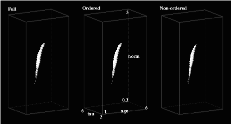
where . Note that the mean and covariance matrix here depend on the parameters - i.e. they are not from the fiducial model. The resultant likelihood is shown in Fig. 4. Clearly it does less well than the full solution, but it does constrain the parameters to a narrow ridge, on which the true solution (age model=100, lies.

The second eigenvector is obtained by taking the normalisation as the second parameter. The vector is shown in the lower panel of Fig. 3. The normalisation parameter is rather a special case, which results in differing from only by a constant offset in the weights (For this parameter and so . The likelihood for the parameters with as the single datum is shown in Fig. 5. On its own, it does not tightly constrain the parameters, but when combined with , it does remarkably well (Fig. 6).


4.1 Three-parameter estimation
We complicate the situation now to a 3-parameter star-formation rate , and estimate , and . Chemical evolution is included by using a simple closed-box model (with instantaneous recycling; ?). This affects the depths of the absorption lines. If we follow the same procedure as before, choosing () as the order for computing , and , then the product of the likelihoods from , and is as shown in the right panel of Fig. 7. The left panel shows the likelihood from the full dataset of 1000 numbers, which does little better than the 3 compressed numbers. It is interesting to explore how the parameter eigenvector method fares in this case. Here we follow the procedure in section 2, and maximise the curvature along the ridge first. The resulting three numbers constrain the parameters as in the middle panel; in this case there is no apparent improvement over using eigenvectors from , but it may be advantageous in other applications.
4.2 Estimate of increase in errors
For the noise model we have adopted, we can readily compute the increase in the conditional error for one of the parameters - the normalisation of the spectrum. This serves as an illustration of how much information is lost in the compression process. In this case, , and , and the Fisher matrix (a single element) can be written in terms of the total number of photons and the number of spectral pixels. From (5), . The compressed data, on the other hand, have a Fisher matrix , so the error bar on the normalisation is increased by a factor
| (18) |
for , and is the average number of photons per pixel. Even if is as low as 2, we see that the error bar is increased only by around 12%.
4.3 Computational issues
We have reduced the likelihood problem in this case by a factor of more than a hundred. The eigenproblem is trivial to solve. The work to be done is in reducing a whole suite of model spectra to numbers, and by forming scalar products of them with the vectors . This is a one-shot task, and trivial in comparison with the job of generating the models.
4.4 Role of fiducial model
The fiducial model sets the weightings . After this step, the likelihood analysis is correct for each , even if the fiducial model is wrong. The only place where there is an approximation is in the multiplication of the likelihoods from all to estimate finally the parameters. The are strictly only uncorrelated if the fiducial model coincides with the true model. This approximation can be dropped, if desired, by computing the correlations of the for each model tested. We have explored how the fiducial model affects the recovered parameters, and an example result from the two-parameter problem is shown in Fig. 8. Here the ages and normalisations of a set of ‘true’ galaxies with S/N are estimated, using a common (9Gyr) galaxy as the fiducial model. We see that the method is successful at recovering the age, even if the fiducial model is very badly wrong. There are errors, of course, but the important aspect is whether the compressed data do significantly worse than the full dataset of 352 numbers. Fig. 8 shows that this is not the case.
Although it appears from this example to be unnecessary, if one wants to improve the solution, then it is permissible to iterate, using the first estimate as the fiducial model. This adds to the computational task, but not significantly; assuming the first iteration gives a reasonable parameter estimate, then one does not have to explore the entire parameter space in subsequent iterations.

5 Comparison with Principal Component Analysis
It is interesting to compare with other data compression and parameter estimation methods. For example, Principal Component Analysis is another linear method (e.g. ?, ?, ?, ?,?, ?, ?, ?, ?, ?, ?, ?), which projects the data onto eigenvectors of the covariance matrix, which is determined empirically from the scatter between flux measurements of different galaxies. Part of the covariance matrix in PCA is therefore determined by differences in the models, whereas in our case refers to the noise alone. PCA then finds uncorrelated projections which contribute in decreasing amounts to the variance between galaxies in the sample.
One finds that the first principal component is correlated with the galaxy age (?). Figure 9 shows the PCA eigenvectors obtained from a set of 20 burst model galaxies which differ only in age, and Figure 10 shows the resultant likelihood from the first two principal components. In the language of this paper, the principal components are correlated, so the covariance matrix is used to determine the likelihood. We see that the components do not do nearly as well as the parameter eigenvectors; they do about as well as on its own. For interest, we plot the first principal component and vs. age in Figure 11. In the presence of noise ( per bin), is almost monotonic with age, whereas PC1 is not. Since PCA is not optimised for parameter estimation, it is not lossless, and it should be no surprise that it fares less well than the tailored eigenfunctions of section III. If one cannot model the effect of the parameters a priori, then this method cannot be used, whereas PCA might still be an effective tool.


6 Discussion
We have presented a linear data compression algorithm for estimation of multiple parameters from an arbitrary dataset. If there are parameters, the method reduces the data to a compressed dataset with members. In the case where the noise is independent of the parameters, the compression is lossless; i.e. the data contain as much information about the parameters as the entire dataset. Specifically, this means the mean likelihood surface around the peak is locally identical whichever of the full or compressed dataset is used as the data. It is worth emphasising the power of this method: it is well known that, in the low-noise limit, the maximum likelihood parameter esimates are the best unbiased estimates. Hence if we do as well with the compressed dataset as with the full dataset, there is no other method, linear or otherwise, which can improve upon our results. The method can result in a massive compression, with the degree of compression given by the ratio of the size of the dataset to the number of parameters. Parameter estimation is speeded up by the same factor.
Although the method is lossless in certain circumstances, we believe that the data compression can still be very effective when the noise does depend on the model parameters. We have illustrated this using simulated galaxy spectra as the data, where the noise comes from photon counting (in practice, other sources of noise will also be present, and possibly dominant); we find that the algorithm is still almost lossless, with errors on the parameters increasing typically by a factor , where is the average number of photons per spectral channel. The example we have chosen is a more severe test of the algorithm than real galaxy spectra; in reality the noise may well be dominated by factors external to the galaxy, such as detector read-out noise, sky background counts (for ground-based measurements) or zodiacal light counts (for space telescopes). In this case, the noise is indeed independent of the galaxy parameters, and the method is lossless.
The compression method requires prior choice of a fiducial model, which determines the projection vectors . The choice of fiducial model will not bias the solution, and the likelihood given the individually can be computed without approximation. Combining the likelihoods by multiplication from the individual is approximate, as their independence is only guaranteed if the fiducial model is correct. However, in our examples, we find that the method correctly recovers the true solution, even if the fiducial model is very different. If one is cautious, one could always iterate. There are circumstances where the choice of a good fiducial model may be more important, if the eigenvectors depend very sensitively on the model parameters. An example of this is the determination of the redshift of the galaxy, whose observed wavelengths are increased by a factor by the expansion of the Universe. If the main signal for comes from spectral lines, then the method will give great weight to certain discrete wavelengths, determined by the fiducial . If the true redshift is different, these wavelengths will not coincide with the spectral lines. It should be stressed that the method will still allow an estimate of the parameters, including , but the error bars will not be optimal. This may be one case where applying the method iteratively may be of great value.
We have compared the parameter estimation method with another linear compression algorithm, Principal Component Analysis. PCA is not lossless unless all principal components are used, and compares unfavourably in this respect for parameter estimation. However, one requires a theoretical model for the methods in this paper; PCA does not require one, needing instead a representative ensemble for effective use. Other, more ad hoc, schemes consider particular features in the spectrum, such as broad-band colours, or equivalent widths of lines (?). Each of these is a ratio of linear projections, with weightings given by the filter response or sharp filters concentrated at the line. There may well be merit in the way the weightings are constructed, but they will not in general do as well as the optimum weightings presented here. It is worth remarking on the ability of the method to separate parameters such as age and metallicity, which often appear degenerately in some methods. In the ‘external noise’ case, then provided the degeneracy can be lifted by maximum likelihood methods using every pixel in the spectrum, then it can also be lifted by using the reduced data. Of course, if the modelling is not adequate to estimate the parameters using all the data, then compression is not going to help at all, and one needs to think again. For example, a complication which may arise in a real galaxy spectrum is the presence of features not in the model, such as emission lines from hot gas. These can be included if the model is extended by inclusion of extra parameters. This problem exists whether the full or compressed data are used. Of course, we can use standard goodness-of-fit tests to determine whether the data are consistent with the model as specified, or whether more parameters are required.
The data compression to a handful of numbers offers the possibility of a classification scheme for galaxy spectra. This is attractive as the numbers are connected closely with the physical processes which determine the spectrum, and will be explored in a later paper. An additional realistic aim is to determine the star formation history of each individual galaxy, without making specific assumptions about the form of the star formation rate. The method in this paper provides the means to achieve this.
Acknowledgments
We thank Andy Taylor and Rachel Somerville, and the referee, Paul Francis, for useful comments. Computations were made using Starlink facilities.
Appendix
In this appendix, we prove that the linear compression algorithm for estimation of an arbitrary number of parameters is lossless, provided the noise is independent of the parameters, . Specifically, loss-free means the Fisher matrix for the set of numbers is identical to the Fisher matrix of the original dataset :
| (19) |
By construction, the are uncorrelated, so the likelihoods multiply and the Fisher matrix for the set is the sum of the derivatives of the log-likelihoods from the individual :
| (20) |
From (7),
| (21) |
With (14), we can write
| (22) |
Hence
Consider first :
proving that these terms are unchanged after compression. We therefore need to consider for or . First we note that
| (25) |
and, from (LABEL:Fam),
| (26) |
We want the sum to extend to . However, the terms from to are all zero. This can be shown as follows: (25) shows that it is sufficient to show that if . Setting in (26), and reversing and , we get
| (27) |
Now, the contribution from does not depend on derivatives wrt higher-numbered parameters, so we can evaluate by setting . The sum (27) implies that this term zero. Increasing successively by one up to , and using (27), proves that all the terms are zero, proving that the compression is lossless.
References
- [Ballinger et al.¡2000¿] Ballinger W. E., Taylor A. N., Heavens A. F., Tadros H., 2000. MNRAS, in preparation.
- [Bond, Jaffe & Knox¡1997¿] Bond J. R., Jaffe A. H., Knox L., 1997. astro-ph, 9708203.
- [Bromley et al.¡1998¿] Bromley B., Press W., Lin H., Kirschner R., 1998. ApJ, 505, 25.
- [Connolly & Szalay¡1999¿] Connolly A., Szalay A., 1999. AJ, 117, 2052.
- [Connolly et al.¡1995¿] Connolly A., Szalay A., Bershady M., Kinney A., Calzetti D., 1995. AJ, 110, 1071.
- [Folkes et al.¡1999¿] Folkes S., Ronen S., Price I., Lahav O., Colless M., Maddox S. J., Deeley K. E., Glazebrook K., Bland-Hawthorn J., Cannon R. D., Cole S., Collins C. A., Couch W., Driver S. P., Dalton G., Efstathiou G., Ellis R. S., Frenk C. S., Kaiser N., Lewis I. J., Lumsden S. L., Peacock J. A., Peterson B. A., Sutherland W., Taylor K., 1999. MNRAS, 308, 459.
- [Folkes, Lahav & Maddox¡1996¿] Folkes S., Lahav O., Maddox S., 1996. MNRAS, 283, 651.
- [Francis et al.¡1992¿] Francis P., Hewett P., Foltz C., Chaffee F., 1992. ApJ, 398, 476.
- [Galaz & deLapparent¡1998¿] Galaz G., de Lapparent V., 1998. A& A, 332, 459.
- [Glazebrook, Offer & Deeley¡1998¿] Glazebrook K., Offer A., Deeley K., 1998. ApJ, 492, 98.
- [Kendall & Stuart¡1969¿] Kendall M. G., Stuart A., 1969. The Advanced Theory of Statistics, London: Griffin.
- [Koch¡1999¿] Koch K., 1999. Parameter Estimation and Hypothesis Testing in Linear Models, Springer-Verlag (Berlin).
- [Murtagh & Heck¡1987¿] Murtagh F., Heck A., 1987. Multivariate data analysis, Astrophysics and Space Science Library, Reidel, Dordrecht.
- [Pagel¡1997¿] Pagel B., 1997. Nucleosynthesis and Chemical Evolution of Galaxies, Cambridge University Press, Cambridge.
- [Ronen, Aragon-Salamanca & Lahav¡1999¿] Ronen R. T., Aragon-Salamanca A., Lahav O., 1999. MNRAS, 303, 284.
- [Singh, Gulati & Gupta¡1998¿] Singh H., Gulati R., Gupta R., 1998. MNRAS, 295, 312.
- [Sodre & Cuevas¡1996¿] Sodre H., Cuevas L., 1996. MNRAS, 287, 137.
- [Tegmark, Taylor & Heavens¡1997¿] Tegmark M., Taylor A., Heavens A., 1997. ApJ, 480, 22.
- [Tegmark¡1997a¿] Tegmark M., 1997a. ApJ(Lett), 480, L87.
- [Tegmark¡1997b¿] Tegmark M., 1997b. Phys. Rev. D, 55, 5895.
- [Worthey¡1994¿] Worthey G., 1994. ApJSS, 95, 107.