ORFEUS II echelle spectra:
deuterium and molecular hydrogen in the ISM towards BD +39 3226

Abstract

In ORFEUS II spectra of the sdO star BD +39 3226 interstellar hydrogen and deuterium is detected. From Ly $\alpha$ profile fitting and a curve of growth analysis of the Lyman series of H i and D i we derive the column densities $N_{\rm H}=1.20^{+0.28}_{-0.22}{\cdot}10^{20}$ cm^-2 and $N_{\rm D}=1.45^{+0.50}_{-0.38}{\cdot}10^{15}$ cm^-2. From the analysis of metal absorption lines in ORFEUS and IUE spectra we obtain column densities for 11 elements. In addition, we examine absorption lines of H₂ for rotational excitation states up to $J=7$. We find an H₂ ortho-to-para ratio of 2.5, the fractional abundance of molecular hydrogen has a low value of $\log f=-4.08$ for a total amount of $N(\mbox{H}_{2})=4.8^{+2.0}_{-1.6}{\cdot}10^{15}$cm^-2. The column densities of the excitation states reveal a moderate Boltzmann excitation temperature of $130$ K and an equivalent excitation temperature for the excited upper states due to UV pumping of $<1800$ K.

1 Introduction

The deuterium abundance in the Galaxy has been of interest since the first models of primordial nucleosynthesis were developed. While it is unlikely that major amounts of deuterium could be produced after the Big Bang, it is sure that deuterium is almost completely destroyed in stars. This should lead to a decrease of its abundance in the progress of galactic evolution. Every measurement of $D/H$ thus should give a lower limit for the primordial abundance and, according to nucleosynthesis models, an upper limit for the baryonic density in the universe. Today, these limits are set by measurements in quasar spectra. For example Levshakov et al. (lev (1999)) suggest a uniform $D/H\simeq 4{\cdot}10^{-5}$ for three lines of sight at redshifts of $z$ between $0.7$ and $3.6$, but Molaro et al. (mola (1999)) find $1.5\cdot 10^{-5}$ from a line of sight with $z=3.5$. Nevertheless knowledge of abundances in the galactic ISM can be important for tracing the evolution of the Milky Way.

Since the Copernicus satellite in the 1970s no instrument was capable of high resolution spectroscopy in the $900$ to $1200$ Å range. There have been $D/H$ measurements with the IUE and the HST-GHRS, but only the Ly $\alpha$ line was observable leading to a restriction to lines of sight with low hydrogen column densities. For an overview see e.g. Lemoine et al. (lemo (1999)).

The ASTRO-SPAS space shuttle platform housed 3 spectrographs operating between $900$ and $1200$ Å. Of those, IMAPS has an echelle spectrograph working between $930$ and $1150$ Å with a resolution of $\lambda/{\Delta\lambda}\simeq 1.5\cdot 10^{5}$. Jenkins et al. (jenk2 (1999)) and Sonneborn et al. (sonne (1999)) performed $D/H$ measurements with that instrument. Two spectrographs were attached to the ORFEUS telescope. The Berkeley spectrograph is designed for intermediate-resolution spectra in the range of $390$ to $1220$ Å. The Heidelberg-Tübingen  echelle spectrograph, equipped with a microchannel plate detector, gives spectra from $912$ to $1410$ Å and allows investigations of the entire hydrogen and deuterium Lyman series with a resolution of $\lambda/{\Delta\lambda}\,{\simeq}\,10^{4}$ (Krämer et al. kraem (1990)). We use spectra of the latter to investigate deuterium.

The large number of rotational transitions of molecular hydrogen found in the wavelength range from 1200 Å  up to the Lyman edge can be used for studies on the molecular gas along the line of sight. The distribution of molecular hydrogen in the local interstellar medium especially at higher galactic latitudes is still only rudimentarily known, since the majority of the Copernicus measurements pointed towards luminous targets in the galactic plane. From the H₂ transitions column densities of the different H₂ rotational excitation states up to $J=7$ can be determined. These can be used to derive physical parameters as the excitation temperature and the ortho-to-para ratio of the molecular hydrogen.

2 Observations and data reduction

BD +39 3226 is a sdO star displaying a pure helium line spectrum in the optical (Giddings gidd (1980)) in a distance of about 270 pc at the galactic coordinates $l=65.00$, $b=+28.77$. Its high radial velocity of $\simeq-$279 km s^-1 makes this star suitable for studies of the local ISM, since stellar and interstellar absorption lines are well separated. We analyse echelle spectra obtained during the ORFEUS II mission in Nov./Dec. 1996 and NEWSIPS reduced long- and short-wavelength high dispersion spectra taken from the IUE Final Archive (IUEFA). The total wavelength range thus covered is about 900 to 3200 Å.

The ORFEUS spectrum was obtained in 4 pointings with a total of $5000$ s integration time. The basic reduction of the data was performed by the ORFEUS team in Tübingen. Details about the ORFEUS instrumentation and the basic data handling and calibration are given in Barnstedt et al. (barn (1999)). We repeat the main features here.

The wavelength calibration of the ORFEUS spectra is based on the interstellar spectrum in the ORFEUS target HD 93521. The accuracy of this calibration is estimated as better than $0.05$ Å, but small systematic effects within the spectrum cannot be excluded. The zero point of the wavelength calibration is based on the geocoronal Ly $\alpha$ emission. Since the ORFEUS aperture measures 20^′′ in diameter, errors in the pointing may shift the wavelength zero point. Optical spectra of BD +39 3226 give the stellar heliocentric radial velocity as $-278.7\pm 5$ km s^-1, based on values by Dworetsky et al. (dwor (1982)) and Giddings (gidd (1980)) and one derived from observations with FOCES at the Calar Alto $2.2$ m telescope. In the ORFEUS spectrum the mean radial velocity of $22$ sharp stellar metal lines is $-289.1\pm 1.5$ km s^-1. We corrected the ORFEUS spectrum for this shift. The new velocity zero point should be accurate within $\approx 5$ km s^-1.

The spectral resolution is intrinsically better than 10⁴, but pointing jitter ($\simeq 2^{\prime\prime}$) and the addition of spectra from several pointings may cause some deterioration. We have filtered the spectra as provided by Tübingen with a wavelet algorithm (Fligge & Solanki 1997) effectively leading to a 3 pixel boxcar filter. We derive from our spectrum a resolution of $\lambda/\Delta\lambda\simeq 0.9{\cdot}10^{4}$.

ORFEUS spectra are influenced by scattered light, which is implicitly corrected for by subtracting the intensities in the interorder space from the echelle order intensities. Near strong features residual effects may still be present (Barnstedt et al. barn (1999)). However, since the ORFEUS spectra are slightly tilted with respect to the detector grid, affected areas lie normally at some distance from such features.

The resolution of the IUE spectra is also about $10^{4}$, which is equivalent to ${\simeq}30\leavevmode\nobreak\$km s^-1. While only one long wavelength spectrum (LWR 11789, exp. time 5040 s) can be found in the IUEFA, several short wavelength spectra are available (SWP 15275, 48312, 48313, 48314, each with 3600 s exp. time). To improve the S/N ratio we added the four SWP spectra. The IUE spectra were smoothed with a 3 pixel boxcar filter.

3 Column densities

3.1 Data analysis

We identified numerous interstellar absorption lines of H i, D i, different heavy elements and H₂. In the photospheric spectrum only a few weak, sharp metal lines of C iii, C iv, N iii, N v, Si iii, Si iv, P v, and S v can be identified besides the strong He ii lines. The investigations on interstellar metal and deuterium abundances make use of the standard curve of growth technique. Except for the case of the Ly ${\alpha}$ and ${\delta}$ absorptions, the equivalent widths of the lines were measured either by a trapezium or by a Gaussian fit. The differences between the two methods are well below the typical errors in the equivalent widths. Uncertainties in the measurements occur because of noise and the choice of the continuum. The error due to the latter was estimated by determining the equivalent width for a lower and an upper limit of the continuum level, the photon statistics were taken into consideration by a formula adopted from Jenkins et al. (jenk (1973)). Both errors added quadratically give the uncertainties in $W_{\lambda}$ as quoted in Tables 1, 3, and 4.

Some lines of S ii, Si ii, and N i, which lie between 1190 and 1390 Å, were measured in both the IUE and the ORFEUS spectrum. The line profiles and absorption strengths turn out to be consistent.

3.2 Metals

Figure 1: Profiles of metal absorption lines in the IUE LWR, IUE SWP, and the ORFEUS spectrum. The velocity components (heliocentric) at $v_{\rm rad}\simeq-75$ km s^-1 (B) and $v_{\rm rad}\simeq-24$ km s^-1 (A) are labeled

Table 1: Metal absorption line equivalent widths measured in component A (at  $v_{\rm rad}\simeq-24$ km s^-1) with ORFEUS and IUE

Ion	Wavelength	$\log(f\lambda)$	Wλ (ORFEUS)	Wλ (IUE)
	[Å]		[mÅ]	[mÅ]
Fe ii	$1096.8769$	$1.545$	$25.6\pm\hskip 4.83691pt8.0$	–
	$1125.4477$	$1.092$	$12.8\pm\hskip 4.83691pt6.4$	–
	$1144.9379$	$2.080$	$64.1\pm\hskip 4.83691pt6.9$	–
	$1608.4511$	$1.998^{*}$	–	$112.1\pm 18.8$
	$2344.214$	$2.410$	–	$161.9\pm 16.4$
	$2374.4612$	$1.889^{*}$	–	$101.4\pm 15.8$
	$2382.039$	$2.967$	–	$163.9\pm 15.9$
	$2586.6500$	$2.248^{*}$	–	$161.3\pm 26.7$
	$2600.1729$	$2.765$	–	$189.1\pm 20.8$
Si ii	$989.8731$	$2.119$	$66.0\pm 15.5$	–
	$1190.4158$	$2.474$	$80.2\pm 11.1$	$79.4\pm\hskip 4.83691pt7.9$
	$1193.2897$	$2.775$	$101.1\pm 10.0$	$94.5\pm\hskip 4.83691pt7.1$
	$1260.4221^{a}$	$3.104$	$98.8\pm 16.4$	$92.9\pm 11.4$
	$1304.3702$	$2.050{{}^{*}}$	$69.6\pm 15.2$	$70.9\pm\hskip 4.83691pt6.5$
	$1526.7066$	$2.225{{}^{*}}$	–	$105.4\pm\hskip 4.83691pt8.1$
	$1808.0126$	$0.596{{}^{*}}$	–	$33.3\pm\hskip 4.83691pt8.4$
Si iii	$1206.500$	$3.311$	$69.6\pm 10.9$	$64.0\pm 12.9$
N i	$964.6256$	$1.059$	$31.2\pm\hskip 4.83691pt8.7$	–
	$1134.9803$	$1.660$	$68.5\pm 10.2$	–
	$1199.5496$	$2.202$	$115.2\pm 10.4$	$80.0\pm\hskip 4.83691pt5.2$
	$1200.2233$	$2.026$	$82.1\pm\hskip 4.83691pt7.6$	$62.5\pm\hskip 4.83691pt7.8$
	$1200.7098$	$1.725$	$54.9\pm\hskip 4.83691pt9.2$	$70.5\pm\hskip 4.83691pt9.6$
O i	$924.952$	$0.168$	$49.4\pm 16.7$	–
	$936.6295$	$0.544$	$67.2\pm 11.9$	–
	$950.8846$	$0.174$	$57.7\pm\hskip 4.83691pt7.0$	–
	$976.4481$	$0.508$	$65.1\pm 11.1$	–
	$1039.2304$	$0.980$	$70.4\pm\hskip 4.83691pt9.7$	–
	$1302.1685$	$1.804$	$b$	$b$
C i	$1277.2454$	$2.091$	–	$20.5\pm\hskip 4.83691pt3.4$
	$1560.3092$	$2.099$	–	$23.4\pm\hskip 4.83691pt8.8$
	$1656.9283$	$2.367$	–	$45.9\pm\hskip 4.83691pt7.7$
C ii	$1036.3367$	$2.124$	$94.4\pm 10.7$	–
	$1334.5323$	$2.235$	$134.0\pm 15.6$	$142.4\pm\hskip 4.83691pt4.0$
S ii	$1250.584$	$0.834$	$34.2\pm 10.0$	$36.3\pm\hskip 4.83691pt5.4$
	$1253.811$	$1.135$	$22.2\pm\hskip 4.83691pt7.5$	$46.4\pm\hskip 4.83691pt6.3$
	$1259.519$	$1.311$	$50.0\pm 10.9$	$59.2\pm\hskip 4.83691pt8.0$
Mg i	$2852.9642$	$3.718$	–	$79.9\pm 17.1$
Mg ii	$2796.352$	$3.235$	–	$239.7\pm 14.9$
	$2803.531$	$2.934$	–	$250.6\pm 20.6$
Mn ii	$2576.877$	$2.956$	–	$56.7\pm 11.2$
	$2594.499$	$2.847$	–	$51.9\pm 13.0$
Ni ii	$1370.132$	$2.254$	–	$6.9\pm\hskip 4.83691pt5.0$
	$1741.549$	$2.256$	–	$14.5\pm\hskip 4.83691pt5.8$
Zn ii	$2026.136$	$2.996^{*}$	–	$43.9\pm 14.2$
	$2062.664$	$2.723^{*}$	–	$10.3\pm\hskip 4.83691pt6.9$
Al ii	$1670.7874$	$3.486$	–	$92.0\pm\hskip 4.83691pt6.7$

Wavelengths and $f$-values are from Morton (mor (1991)), except for   ^∗ taken from Savage & Sembach (sav:sem (1996))
^a Line blended with Fe ii at $1260.533$ Å. The equivalent width given here has already been corrected for a contribution of $31.5\pm 4.6$ mÅ derived from the determined Fe ii column density
$b$ The $1302$ O i line is in ORFEUS spectra blended with geocoronal O i emission, in IUE spectra with a reseaux

Table 2: Metal column densities $N$ [cm^-2] and abundances. Solar values are taken from de Boer et al. (boer (1987))

Element	$\log N$	$\log(N/N_{\rm H})$	$\log(N/N_{\rm H})_{\sun}$
C	$16.40\,\pm 0.75$	$-3.70\,\pm 0.75$	$-3.4$
N	$14.75\,\pm 0.25$	$-5.35\,\pm 0.25$	$-4.0$
O	$16.40\,^{+0.75}_{-0.50}$	$-3.70\,^{+0.75}_{-0.50}$	$-3.16$
Mg	$14.95\,\pm 0.80$	$-5.15\,\pm 0.80$	$-4.46$
Al	$13.00\,^{+0.40}_{-0.35}$	$-7.10\,^{+0.40}_{-0.35}$	$-5.6$
Si	$14.80\,\pm 0.20$	$-5.30\,\pm 0.20$	$-4.45$
S	$14.80\,\pm 0.20$	$-5.30\,\pm 0.20$	$-4.8$
Mn	$12.60\,\pm 0.10$	$-7.50\,\pm 0.15$	$-6.58$
Fe	$14.10\,\pm 0.15$	$-6.00\,\pm 0.15$	$-4.50$
Ni	$12.65\,\pm 0.30$	$-7.45\,\pm 0.30$	$-5.72$
Zn	$12.40\,\pm 0.30$	$-7.70\,\pm 0.30$	$-7.4$

In order to judge the velocity structure of the absorption it is reasonable to analyze the metal lines at first. We find 2 different absorption components: one at a radial velocity (heliocentric) of ${\simeq-24}$ km s^-1 (component A) and one at $\simeq-75$ km s^-1 (component B). The latter is rather weak, Si ii equivalent widths are smaller than 24 mÅ with large uncertainties, so an examination of component B can give only very uncertain results. Even if this component had a very low $b$-value, the upper limits for the S ii and Si ii column densities would be roughly $1.6{\cdot}10^{14}$ cm^-2 and $7.9{\cdot}10^{14}$ cm^-2 respectively corresponding to a hydrogen column density of $\leq 10^{19}$ cm^-2 .

In the following we will concentrate on the cloud at $-24$ km s^-1. The small LSR velocity of this component suggests a local origin while component B at $-75$ km s^-1 represents most likely a cloud at larger distance.

Table 1 lists the measured equivalent widths for component A. The lines of Fe ii, Si ii, and N i were used to determine the $b$-value of 5$\pm$1 km s^-1 of the curve of growth for metals. Then column densities of other ions were obtained by fitting their equivalent width to the curve. Fig. 2 shows the curve of growth, Table 2 gives the resulting column densities. The errors take the uncertainties in the $b$-value and in the individual equivalent widths into account. For ions with data points only in the flat part of the curve of growth the column densities have large uncertainties.

Figure 2: The curve of growth for absorption by metals on the line of sight to BD~+39 3226 (component A) is shown. Plotted are only Si ii, Fe ii, and N i which actually define the curve of growth. Filled symbols represent ORFEUS data, open symbols those from the IUE. The drawn curves represent single cloud absorption with indicated $b$-value

3.3 Neutral hydrogen

Figure 3: The curve of growth for H i and D i towards BD~+39 3226. In the damping part the curves split, the lower curve is for Ly $\kappa$, the upper one is for Ly $\delta$. Note that the D i points lie essentially on the Doppler part of the curve of growth

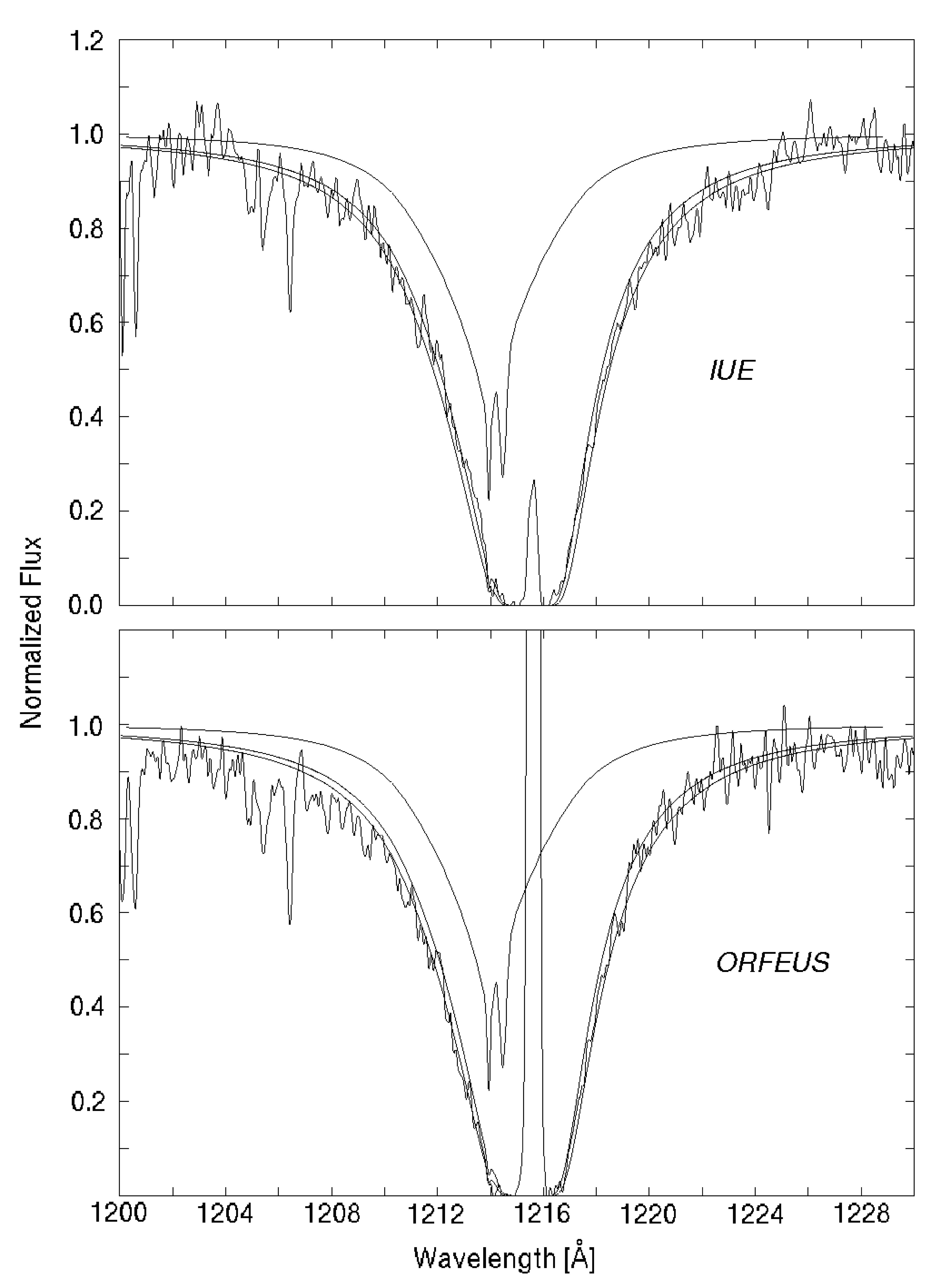
Figure 4: Theoretical fits to the Lyman $\alpha$ line in the IUE and the ORFEUS spectrum. In both spectra the residual intensity near the centre of the absorption has been set to zero. The contribution of the stellar He ii line located $\simeq 1.57$ Å towards shorter wavelengths as calculated from an atmospheric model is included in the fits and plotted seperately. The two shown fits represent $\log N$(H i)$=20.0$ and $20.1$. Near the centre the geocoronal emission peak is visible

Figure 5: Curve of growth for H i in detail. The data points and the corresponding theoretical curves are labeled

Figure 6: The Lyman lines used in our curve of growth analysis in the ORFEUS spectrum. The positions of D and H absorption by component A ($v_{\rm rad}\simeq-24$) are marked

We determined the H i column density in two different ways.

First we compared theoretical Voigt profiles convolved with a gaussian instrumental profile to the Ly ${\alpha}$ line in the ORFEUS and the IUE spectrum. This line is always fully damped, therefore the $b$-value is unimportant and in case of a single velocity component only the column density remains as a parameter. Even small changes in the column density have a clear effect on the profile. We estimate the accuracy in $\log N$ as $\pm 0.1$. Problems arise because of the weaker component B at $\Delta\lambda{\simeq}-0.21$ Å and stellar He ii absorption at $\Delta\lambda{\simeq}-1.57$ Å which both are unresolved. Component B should have only a weak influence on the column density, probably $\leq 0.04$ dex. The stellar line was calculated from an atmospheric model ($T_{\rm eff}=45000$ K, $\log g=5.5$, $n$(He)$=99$%, $n$(H)$=1$%) and included in the fit. The uncertainty in $N$(H i) due to the stellar model is small, because significant errors in the strength of the calculated stellar line would have made the fit profile asymmetric with regard to the measured profile. An additional background substraction was applied in both spectra of the Lyman $\alpha$ line to correct for some residual intensity ($\approx 5.5$% in the ORFEUS spectrum) near the centre. The result is plotted in Fig. 4. It is only possible to give a total column density (for component A and B), which is $N_{\rm H}=1.12^{+0.29}_{-0.23}{\cdot}10^{20}$ cm^-2.

Table 3: Hydrogen and deuterium equivalent widths. Wavelengths and oscillator strengths are taken from Morton (mor (1991)). H i and D i Ly $\epsilon$ have been corrected for the influence of Fe ii absorption at 937.652 Å, H i and D i Ly $\zeta$ for the influence of the H₂ We Q(1), 4-0 line at 930.574 Å

Ion	Lyman line	Wavelength [Å]	$\log f{\lambda}$	$W_{\lambda}$ [mÅ]
H i	$\delta$	$949.7431$	$1.122$	$337.0\pm 20.1$
	$\epsilon$	$937.8035$	$0.864$	$218.0\pm 21.0$
	$\zeta$	$930.7483$	$0.651$	$240.3\pm 18.9$
	$\eta$	$926.2257$	$0.470$	$222.8\pm 17.0$
	$\kappa$	$919.3514$	$0.043$	$202.1\pm 21.5$
D i	$\delta$	$949.4847$	$1.122$	$84.6\pm 10.0$
	$\epsilon$	$937.5484$	$0.865$	$47.2\pm 17.5$
	$\zeta$	$930.4951$	$0.651$	$24.8\pm 16.1$
	$\eta$	$925.9737$	$0.470$	$24.4\pm 11.7$
	$\kappa$	$919.101\,^{*}$	$0.043$	$<30.7$

^∗ Wavelength calculated from H i Ly $\kappa$.

To confirm this value, we also applied the curve-of-growth analysis to the Lyman series from Ly ${\delta}$ to Ly ${\kappa}$, except for Ly ${\theta}$ and Ly ${\iota}$ which seem distorted. The Ly $\beta$ and Ly $\gamma$ lines have strong damping wings which, together with the further structure of the spectrum, do not allow the determination of reliable equivalent widths. Higher Lyman lines are also visible but may be blended with stellar He ii, because the distance between these lines is smaller than the stellar radial velocity. Besides, near the Lyman edge it is not possible to set the continuum properly. We measured the equivalent width of Ly ${\delta}$ by comparing the line with computed two-component-profiles (Voigt profiles convolved with the instrumental Gauss profile), one component for the H i and one for the D i line. For the other lines the damping wings are neglegible and we used two-component Gauss fits.

We note that for the higher Lyman series lines ($\delta$-$\kappa$) the instrumental profile degrades the true absorption such that residual light is expected near the bottom of the profiles (see Fig. 6 and 7). A calculation shows this to be at the level of up to $10$%. In addition, also in these lines geocoronal emission is present but not readily recognizable in the profiles considered (in Lyman $\alpha$ and $\beta$ it is clearly present). Since the absolute level of the contamination is not reliably known we have refrained from corrections.

In case of Ly $\epsilon$ the Fe ii line situated between the H i and the D i line at $937.652$ Å was modeled and used as a third, fixed component in the fit. An analogous procedure was necessary for the H₂ Werner Q(1), 4-0 line lying at $\lambda=930.574$ Å between the H i and D i Lyman $\zeta$ lines. Attempts to include velocity component B by additional fit components showed that it has neglegible influence on the line shape. Examples for the fits are shown in Fig. 7. Though the velocity structure is not resolved in the Lyman series, a single-cloud curve of growth should be sufficient since there is one clearly dominant cloud. As expected the H i curve of growth has a significantly higher Doppler-velocity than the metals’ curve due to the much smaller atomic mass of hydrogen. For a given $b$ each measured equivalent width and its error correspond to a column density with an error depending on the slope of the curve of growth. We calculated $\log N_{\rm H}$ for different $b$-values from the weighted mean of the 5 column densities resulting from the 5 measured equivalent widths. The least mean square deviation is found for $b=10.5\pm 1$ km s^-1, leading to $N_{\rm H}=1.6^{+0.9}_{-0.6}{\cdot}10^{20}$ cm^-2. Fig. 3 and 5 show the curve for H i.

Figure 7: For two of the Lyman lines a 500 km s^-1 wide section of the spectrum is displayed. Top: Deuterium and hydrogen Lyman $\delta$ line in the ORFEUS spectrum (data points) with a two-component fit (Voigt profile convolved with instrumental Gauss). Bottom: Deuterium and hydrogen Lyman $\eta$ line (data points) with a two-component Gauss profile. In both plots the positions of the velocity components A and B found in the metal lines are marked for the H i lines. Component B has only neglegible effect on the absorption profile

The Lyman $\alpha$ fit and the curve of growth analysis give consistent results, so a mean value of $N_{\rm H}=1.20^{+0.28}_{-0.22}{\cdot}10^{20}$ cm^-2 can be derived.

3.4 Deuterium

The absorption of deuterium was investigated in 5 lines (see Table 3). The D i Lyman $\delta$ and $\eta$ lines are shown in Fig. 7. Along with the H i data, the D i equivalent widths are plotted in Fig. 3. For D i Ly ${\kappa}$ only an upper limit can be given which is rather high due to the continuum uncertainty. The Doppler parameter is only of minor importance for the determination of the D i column density because the data points lie mainly on the linear part of the curve of growth. The deuterium data points seem to suggest a somewhat higher $b$-value than $10.5$ km s^-1 but we used the same curve as for hydrogen since we expect $b_{\,\rm D}\leq b_{\,\rm H}$. The weighted mean of the column densities derived for $b=10.5$ km s^-1 from the four measured $W_{\lambda}$ values is $N_{\rm D}=1.45^{+0.50}_{-0.38}{\cdot}10^{15}$ cm^-2.

3.5 Molecular hydrogen

The ORFEUS spectra also contain a large number of absorption lines from molecular hydrogen. Only one component is visible here. The average radial velocity of $18$ lines measured in the echelle orders $50$-$59$ is $v_{\rm{helio}}=-27.1\pm{0.9}$ km s^-1, slightly different from the velocity found for the metal absorption lines. The metal radial velocity of $v_{\rm{helio}}=-23.9\pm{1.0}$ km s^-1, was measured as the average value of $20$ lines in the echelle orders $42$-$60$. Since we have not found any obvious systematic velocity shift between different orders, a possible explanation may be the presence of an additional weak unresolved absorption component in the metal lines.

We have determined equivalent widths using trapezium fits. No better quality of the results would be achievable from fitting gaussian profiles since most of the lines are only weak and do not show clear profiles. The equivalent width for rotational states $J\geq 5$ are similar to the strength of noise peaks, so only upper limits are determined. Results are presented in Table 4.

Column densities for the different rotational excitation levels are derived from these equivalent widths by fitting to a theoretical curve of growth (Fig. 9). The $b$-value is restricted by the lower $J$ levels to $2.5$ to 3 km s^-1. The column densities for $J=0$ and $1$ lie in the flat part of the curve of growth and therefore are sensitive to variations of the $b$-value, enlarging the errors for their column densities. The higher rotational levels are located on the doppler part of the curve which in principle allows a good definition of column densities. However, most of these lines are weak and have larger errors in the equivalent widths which again leads to larger errors in the column densities. For $J\geq 5$ only upper limits can be given. The resulting column densities are listed in Table 4.

The population of the lower rotational states of molecular hydrogen is determined by collisional excitation, following a Boltzmann distribution. The excitation temperature can therefore be derived as

$$T_{mn}=\frac{E_{n}-E_{m}}{2.303\,k}\frac{1}{\log\left(N_{m}/g_{m}\right)-\log\left(N_{n}/g_{n}\right)},$$ (1)

where the statistical weight $g_{J}$ is equal to $(2J+1)$, multiplied by a factor of 3 for $J$ odd in regard to the triplet nature of ortho-H₂. For the upper levels UV photons have to be considered as the primary source of excitation (Spitzer & Zweibel spitzer_zweibel (1974); Spitzer et al. spitzer_cochran (1974)). An equivalent excitation temperature can be derived here, but this has by no means the physical implications of an actual kinetic temperature.

We have determined excitation temperatures by using an error weighted least square fit. A temperature of $T_{02}=130\pm 1$ K is derived for the lower levels $J=0$ to $2$, for the upper levels we find an upper limit in the equivalent excitation temperature of $T_{37}<1800$ K.

Figure 8: Overview of the spectra for some H₂ transitions. The spectra shown are filtered by a wavelet algorithm. The H₂ absorption at $v_{\rm{helio}}\simeq-27$ km s^-1 is clearly visible for the transitions with $J\leq 4$. At higher rotational states the equivalent widths are similar to the strength of noise peaks. Additional absorption lines marked are: a) Ly R(1), 2-0; b) Ly R(0), 4-0; c) Ly P(1), 4-0; s) features of probably stellar origin, which could not be unambigiously identified

Looking at Fig. 10, where the column density $N_{J}$, weighted by the statistical weight $g_{J}$, is plotted against the excitation energy of the rotational state $J$, a clear distinction is visible between the collisionally Boltzmann excited levels $J\leq 2$ and the UV photon excited levels $J\geq 3$. Although the upper levels scatter around the fit, a much smaller slope is obvious, compared with the lower levels.

The H₂ ortho-to-para ratio (OPR) derived from the by far most prominent rotational states $J=0$ and $1$ is $N(1)/N(0)\simeq 2.5$. The excitation temperature calculated using the lowest para-states $J=0$ and $2$ is $T_{02}=130$ K. This value essentially coincides with the temperature determined from the OPR of $T_{01}=134$ K. We therefore can assume that we see thermalized, purely collisionally excited gas in the excitation levels up to $J=2$, following the Boltzmann distribution (see Dalgarno et al. dalg (1973)).

For the higher excitation levels information is less clear due to the scatter in the data points. Fitting the ortho- and para-states seperately we get $T_{35}<870$ K and $T_{46}<1400$ K, so the excitation temperature for the upper states probably can be restricted to $<1400$ K rather than $<1800$ K as stated above.

4 Abundances

4.1 Metals, dust, and $H_{2}$

Table 4: H₂ equivalent widths and column densities $N_{J}$ [cm^-2]

Transition	$\lambda$ $\left[\mbox{\AA}\right]$	$f^{a}$	$W_{\lambda}$ $\left[\mbox{m\AA}\right]$	Notesb
$J=0$ $(g_{J}=1,E_{J}=0)$; $\log N_{J}=15.10\pm 0.20$
Ly R(0), 0-0	$1108.128$	$0.00173$	$18.6\pm 4.8$
Ly R(0), 1-0	$1092.194$	$0.00596$	$27.7\pm 4.0$
Ly R(0), 2-0	$1077.138$	$0.0119$	$46.7\pm 6.1$
Ly R(0), 3-0	$1062.883$	$0.0182$	$41.1\pm 6.0$
Ly R(0), 8-0	$1001.826$	$0.0266$	$<34.0$	b
$J=1$ $(g_{J}=9,E_{J}=0.01469)$; $\log N_{J}=15.50^{+0.20}_{-0.30}$
We Q(1), 0-0	$1009.772$	$0.0238$	$53.2\pm 7.1$
Ly R(1), 1-0	$1092.732$	$0.00403$	$22.6\pm 5.1$
We Q(1), 1-0	$986.798$	$0.0364$	$44.7\pm 7.9$
Ly R(1), 2-0	$1077.698$	$0.00809$	$53.2\pm 7.2$
We Q(1), 2-0	$966.097$	$0.0349$	$<56.8$	b
Ly P (1), 3-0	$1064.606$	$0.00584$	$15.6\pm 5.0$
Ly R(1), 4-0	$1049.958$	$0.0160$	$36.1\pm 4.9$
Ly P (1), 7-0	$1013.434$	$0.0205$	$<40.2$	b
$J=2$ $(g_{J}=5,E_{J}=0.04394)$; $\log N_{J}=14.10^{+0.15}_{-0.20}$
We Q(2), 0-0	$1010.941$	$0.0238$	$22.3\pm 6.1$
Ly R(2), 1-0	$1094.244$	$0.00367$	$<10.6$
We Q(2), 2-0	$967.278$	$0.0348$	$15.5\pm 5.5$	n
Ly R(2), 4-0	$1051.497$	$0.0147$	$20.7\pm 4.6$
Ly R(2), 5-0	$1038.690$	$0.0170$	$9.7\pm 3.8$
$J=3$ $(g_{J}=21,E_{J}=0.08747)$; $\log N_{J}=13.95^{+0.15}_{-0.10}$
Ly P (3), 1-0	$1099.788$	$0.00240$	$<5.2$	n
Ly P (3), 3-0	$1070.142$	$0.00721$	$13.2\pm 4.3$
We Q(3), 4-0	$933.581$	$0.0193$	$<13.7$
Ly P (3), 5-0	$1043.498$	$0.0104$	$11.8\pm 3.5$
$J=4$ $(g_{J}=9,E_{J}=0.14491)$; $\log N_{J}=13.80^{+0.30}_{-0.20}$
Ly P (4), 3-0	$1074.313$	$0.00733$	$12.2\pm 3.6$
Ly Q(4), 4-0	$935.959$	$0.0192$	$9.4\pm 5.6$
Ly P (4), 6-0	$1035.184$	$0.0108$	$<11.4$
$J=5$ $(g_{J}=33,E_{J}=0.21575)$; $\log N_{J}<13.40$
We Q(5), 1-0	$994.924$	$0.0361$	$<9.0$
We Q(5), 2-0	$974.286$	$0.0346$	$<10.7$
Ly P (5), 5-0	$1052.499$	$0.0105$	$<3.9$
$J=6$ $(g_{J}=13,E_{J}=0.29940)$; $\log N_{J}<13.40$
Ly R(6), 1-0	$1109.859$	$0.00307$	$<4.1$
Ly P (6), 4-0	$1071.497$	$0.0102$	$<6.8$
Ly R(6), 6-0	$1041.711$	$0.0143$	$<4.8$
Ly P (6), 6-0	$1045.805$	$0.0122$	$<5.9$
Ly R(6), 8-0	$1019.101$	$0.0133$	$<3.7$
$J=7$ $(g_{J}=45,E_{J}=0.39521)$; $\log N_{J}<13.50$
Ly R(7), 5-0	$1059.992$	$0.0134$	$<7.7$
Ly P (7), 6-0	$1052.386$	$0.0123$	$<4.9$
a $f$ values from Morton & Dinerstein (mor:din (1976))
b b: line is possibly blended; n: spectrum has locally small S/N

Figure 9: Curve of growth for the different excitation levels of H₂. Downward arrows denote upper limits for the equivalent width. The $b$-value is based on the absorption in levels $J=0$ to $2$

The metal abundances in component A are given in Table 2. Since only a total hydrogen column density for components A and B could be measured, the abundances may be too low by $\leq 0.04$ dex. In presence of the relatively large uncertainties this effect seems neglegible.

As can be seen in Table 2 the depletion factors $\log\,d=\log(N/N_{\rm H})-\log(N/N_{\rm H})_{\sun}$ of the elements vary between $-0.3$ and $-1.7$. This moderate depletion indicates a low abundance of dust along the line of sight.

The total amount of H₂ seen on this line of sight is $N(\mbox{H}_{2})=4.8^{+2.0}_{-1.6}{\cdot}10^{15}$ cm^-2, which gives an abundance relative to H i of $-4.40^{+0.17}_{-0.20}$ dex. With this low value the total amount of hydrogen, $N(\mbox{H\,{\sc i}}+\mbox{H}_{2})=[N(\mbox{H\,{\sc i}})+2N(\mbox{H}_{2})]=1.2{\cdot}10^{20}$ cm^-2, is hardly larger than the value given above for just H i.

The extinction towards BD +39 3226 is given by Dworetsky et al. (dwor (1982)) as $E(B-V)=0.05$, which again indicates a low dust abundance. In addition, the fractional abundance of molecular hydrogen $f=2N(\mbox{H}_{2})/\left[N(\mbox{H\,{\sc i}})+2N(\mbox{H}_{2})\right]$ has a low value of $\log f=-4.08$. The gas to color excess ratio for our line of sight of $N\left(\mbox{H {\sc i}}+\mbox{H}_{2}\right)/E(B-V)=2.3\cdot 10^{21}$ cm^-2 mag^-1 is slightly lower than the typical value for the galactic intercloud gas of $5.0\cdot 10^{21}$ cm^-2 mag^-1 given by Bohlin et al. (bohlin78 (1978)). This deviation, though, can be explained by uncertainties in the $E(B-V)$ value and should not be overinterpretated. We can conclude that most of the absorption seen on this line of sight arises from intercloud gas with only little contribution from the clouds having $T\simeq 130$ K.

Figure 10: Excitation plot for the H₂ column densities. Plotted is the statistically weighted column density vs. excitation energy of the rotational states. A clear separation of collisionally excited levels ($J\leq 2$) and of UV photon excited levels ($J\geq 3$) is visible. The lines denote least square fits to an assumed Boltzmann distribution for levels $m$ to $n$ with the appropriate temperature $T_{mn}$. The error given for the Boltzmann excitation temperature $T_{02}$ is the standard deviation of the fit. For $T_{37}$ only an upper limit can be given

Savage et al. (savage77 (1977)) have generated a plot of $\log f$ vs. $E(B-V)$ for their survey of $70$ stars. For lines of sight with $E(B-V)<0.08$, they find only very small fractions of H₂ down to values $\log f$ of $-6$. This is in line with the tight connection between the existence of dust grains and of molecules forming on their surfaces. Our low value fits well into this group of stars of low fractional abundance.

In their plot, Savage et al. (savage77 (1977)) show theoretical curves from equilibrium models of Black for different hydrogen densities, radiation densities, and molecule formation rates. According to this, our value is described by Black’s “Model $2$”, which assumes a density $n(\mbox{H\,{\sc i}}+\mbox{H}_{2})$ of 100 cm^-3 at a temperature of about $100$ K, in accordance to the temperature derived above. The radiation density at $1000$ Å has then a value of $4\cdot 10^{-17}$ erg cm^-3 Å^-1 if the molecule formation rate is $10^{-17}$ cm³ s^-1.

4.2 Deuterium

From the H i and D i column densities we obtain a deuterium abundance on this line of sight of $D/H=1.2^{+0.5}_{-0.4}{\cdot}10^{-5}$. We also tried to identify absorption lines of HD, but without success. Taking the H₂ column density of only $4.8{\cdot}10^{15}$ cm^-2 one would expect HD column densities as low as about $10^{11}$ cm^-2, which is definitely below the detection limit of $\simeq 10^{13}$ cm^-2 for the spectra available. It can be ruled out that any significant amount of deuterium is hidden in HD. Deuterium depletion by interactions with dust grains is unlikely in a warm ISM component with low gas-to-dust ratio.

The abundance is a value for the whole line of sight, possibly an average over more than one cloud with different $D/H$ ratios. The uncertainties are rather large, but the value is reliable within its limitations. There was no need for assumptions about the velocity structure of the absorption (as it is necessary for line modelling) since the hydrogen column density determination is mainly based on fully damped absorption while the deuterium lines lie in the linear part of the curve of growth. In both cases the curve of growth is insensitive to effects arising from clouds of different $b$-values and column densities. Furthermore, a model of the stellar spectrum was used only for Lyman $\alpha$ fitting. The uncertainty arising from modelling is neglegible because the centres of the stellar and interstellar absorption lines are well separated due to the high radial velocity of the star.

Varying scattered light may affect the measured equivalent widths, as mentioned in Sect. 2. However, we do not find evidence for systematic background substraction errors beyond the $5$% level in all analyzed H and D lines and the scatter of the equivalent widths is not larger than expected for the estimated errors. The effect of systematic errors would be rather small. For example, if all H and D equivalent widths were larger by $10$ % than measured due to wrong background substraction, the D i column density also would rise by $\approx 10$% while the H i column density resulting from curve of growth analysis and Lyman $\alpha$ fitting would change even less. Thus the $D/H$ ratio would be increased by less than $10$ % and would remain well within the given range.

5 Concluding remarks

McCullough (mccu (1992)) finds all Copernicus and IUE  ISM deuterium abundance measurements to be consistent with $D/H=(1.5\pm 0.2){\cdot}10^{-5}$. This value was confirmed for the local interstellar cloud by GHRS observations towards $α$ Aur (Linsky et al. lins (1995)) and HR 1099 (Piskunov et al. pisk (1997)) yielding $D/H=1.60^{+0.14}_{-0.19}{\cdot}10^{-5}$ and $1.46\pm 0.09{\cdot}10^{-5}$ respectively. For a summary of GHRS measurements see Linsky (lins2 (1998)). McCullough’s list of included data contains $6$ measurements towards nearby stars ($d\,{\leq}\,14$ pc) observed only in Ly $\alpha$ and $8$ Copernicus observations of each $2$ to $5$ Lyman lines towards more distant stars ($d\,{\geq}\,79$ pc). The mean of the results of the latter observations is $D/H\simeq 1.4{\cdot}10^{-5}$. Our result based on 5 deuterium lines lies below this value though it is consistent within its uncertainty.

Recent determinations of $D/H$ for example by Vidal-Madjar et al. (vidmad (1998)) towards G191-B2B using the GHRS ($D/H=1.12_{-0.08}^{+0.08}{\cdot}10^{-5}$), Gölz et al. (golz (1998)) in a preliminary analysis of ORFEUS II observations of BD +28 4211 ($D/H=0.8^{+0.7}_{-0.4}{\cdot}10^{-5}$) or Jenkins et al. (jenk2 (1999)) using IMAPS spectra of $δ$ Ori ($D/H=0.74^{+0.19}_{-0.13}{\cdot}10^{-5}$) indicate smaller values towards early type stars with $d\geq 69$ pc. As Vidal-Madjar et al. and Jenkins et al. state, a possible explanation may be blending of the Local Interstellar Cloud (LIC) contribution with that of more distant deuterium-poor clouds. Small scale spatial inhomogeneities of $D/H$ could be the result of the production of significant amounts of deuterium in stellar flares, as Mullan & Linsky (mul:lin (1999)) suggest. This discussion remains open since Sahu et al. (sahu (1999)) found $D/H=1.60^{+0.39}_{-0.27}\cdot 10^{-5}$ towards G191-B2B from a STIS spectrum, a value consistent with a homogeneous $D/H$ in the LISM.

However this may be, the various determinations of $D/H$ all are consistent with $D/H\approx(1.2\pm 0.3){\cdot}10^{-5}$. The uncertainty in each individual value is influenced by the spectral resolution of the instrument, by the number of D lines used, and by the actual D column density. Our result from the new instrument ORFEUS using $5$ lines at $30$ km s^-1 resolution adds to these determinations .

- (1) Barnstedt J., Kappelmann N., Appenzeller I., et al., 1999, A&AS 134, 561
- (2) Bohlin R.C., Savage B.D., Drake J.F., 1978, ApJ 224, 132
- (3) Dalgarno A., Black J.H., Weisheit J.C., 1973, Ap. Letters 14, 77
- (4) de Boer K.S., Jura M.A., Shull J.M., 1987, in: Scientific Accomplishments of the IUE, ed. Y.Kondo, D. Reidel Publishing Company, 485
- (5) Dworetsky M.M., Whitelock P.A., Carnochan D.J., 1982, MNRAS 201, 901
- (6) Fligge M., Solanki S.K., 1997, A&AS 124, 579
- (7) Giddings J., 1980, PhD Thesis, University College London
- (8) Gölz M., Kappelmann N., Appenzeller I., et al., 1998, in: Proc. IAU Colloq. 166, The Local Bubble and Beyond, eds. D.Breitschwerdt, M.J.Freyberg, & J. Trümper (Springer), 75
- (9) Jenkins E.B., Drake J.F., Morton D.C., et al., 1973, ApJ 181, L122
- (10) Jenkins E.B., Tripp T.M., Woźniak P.R., et al., 1999, ApJ 520, 182
- (11) Krämer G., Barnstedt J., Eberhardt N., et al., 1990, in: IAU Coll. 123, ’Observatories in Earth Orbit and beyond’, ed. Y.Kondo, Kluwer, p. 177
- (12) Lemoine M., Audouze J., Jaffel L.B., et al., 1999, NewA 4, 231
- (13) Levshakov S.A., Tytler D., Burles S., 1999, AJ, submitted (astro-ph/9812114)
- (14) Linsky, J.L., 1998, Space Sci. Rev. 84,285
- (15) Linsky J.L., Diplas A., Wood B.E., et al., 1995, ApJ 451, 335
- (16) McCullough P.R., 1992, ApJ 390, 213
- (17) Molaro P., Bonifacio P., Centurion M., Vladilo G., 1999, A&A 349, L13
- (18) Morton D.C., 1991, ApJS 77, 119
- (19) Morton D.C., Dinerstein H.L., 1976, ApJ 204, 1
- (20) Mullan D.J., Linsky J.L., 1999, ApJ 511, 502
- (21) Piskunov N., Wood B.E., Linsky J.L., et al., 1997, ApJ 474, 315
- (22) Sahu M.S., Landsman W., Bruhweiler F.C. et al., 1999, ApJ 523L, 159
- (23) Savage B.D., Sembach, K.R., 1996, ARA&A 34, 279
- (24) Savage B.D., Bohlin R.C., Drake J.F., Budich W., 1977, ApJ 216, 291
- (25) Sonneborn G., et al., 1999, in preparation (cited in Jenkins et al. 1999)
- (26) Spitzer L., Zweibel E.G., 1974, ApJ 191, L127
- (27) Spitzer L., Cochran W.D., Hirshfeld A., 1974, ApJS 28, 373
- (28) Vidal-Madjar A., Lemoine M., Ferlet R., et al., 1998, A&A 338, 694