TESTING HOMOGENEITY ON LARGE SCALES

Abstract

We review observational tests for the homogeneity of the Universe on large scales. Redshift and peculiar velocity surveys, radio sources, the X-Ray Background, the Lyman-$\alpha$ forest and the Cosmic Microwave Background are used to set constraints on inhomogeneous models and in particular on fractal-like models. Assuming the Cosmological Principle and the FRW metric, we estimate cosmological parameters by joint analysis of peculiar velocities, the CMB, cluster abundance, IRAS and Supernovae. Under certain assumptions the best fit density parameter is $\Omega_{m}=1-\lambda\approx 0.3-0.5$.

Institute of Astronomy, Madingley Road, Cambridge CB3 0HA, UK; and Racah Institue of Physics, The Hebrew University, Jerusalem 91904, Israel (email: lahav@ast.cam.ac.uk)

1. Introduction

The Cosmological Principle was first adopted when observational cosmology was in its infancy; it was then little more than a conjecture, embodying ’Occam’s razor’ for the simplest possible model. Observations could not then probe to significant redshifts, the ‘dark matter’ problem was not well-established and the Cosmic Microwave Background (CMB) and the X-Ray Background (XRB) were still unknown. If the Cosmological Principle turned out to be invalid then the consequences to our understanding of cosmology would be dramatic, for example the conventional way of interpreting the age of the Universe, its geometry and matter content would have to be revised. Therefore it is important to revisit this underlying assumption in the light of new galaxy surveys and measurements of the background radiations.

Like with any other idea about the physical world, we cannot prove a model, but only falsify it. Proving the homogeneity of the Universe is in particular difficult as we observe the Universe from one point in space, and we can only deduce directly isotropy. The practical methodology we adopt is to assume homogeneity and to assess the level of fluctuations relative to the mean, and hence to test for consistency with the underlying hypothesis. If the assumption of homogeneity turns out to be wrong, then there are numerous possibilities for inhomogeneous models, and each of them must be tested against the observations.

Despite the rapid progress in estimating the density fluctuations as a function of scale, two gaps remain:

(i) It is still unclear how to relate the distributions of galaxies and mass (i.e. ‘biasing’); (ii) Relatively little is known about fluctuations on intermediate scales between these of local galaxy surveys ($\sim 100h^{-1}$ Mpc) and the scales probed by COBE ($\sim 1000h^{-1}$ Mpc).

Here we examine the degree of smoothness with scale by considering redshift and peculiar velocities surveys, radio-sources, the XRB, the Ly-$\alpha$ forest, and the CMB. We discuss some inhomogeneous models and show that a fractal model on large scales is highly improbable. Assuming an FRW metric we evaluate the ’best fit Universe’ by performing a joint analysis of cosmic probes.

2. Cosmological Principle(s)

Cosmological Principles were stated over different periods in human history based on philosophical and aesthetic considerations rather than on fundamental physical laws. Rudnicki (1995) summarized some of these principles in modern-day language:

$\bullet$ The Ancient Indian: The Universe is infinite in space and time and is infinitely heterogeneous.

$\bullet$ The Ancient Greek: Our Earth is the natural centre of the Universe.

$\bullet$ The Copernican CP: The Universe as observed from any planet looks much the same.

$\bullet$ The Generalized CP: The Universe is (roughly) homogeneous and isotropic.

$\bullet$ The Perfect CP: The Universe is (roughly) homogeneous in space and time, and is isotropic in space.

$\bullet$ The Anthropic Principle: A human being, as he/she is, can exist only in the Universe as it is.

We note that the Ancient Indian principle can be viewed as a ‘fractal model’. The Perfect CP led to the steady state model, which although more symmetric than the PC, was rejected on observational grounds. The Anthropic Principle is becoming popular again, e.g. in explaining a non-zero cosmological constant. Our goal here is to quantify ’roughly’ in the definition of the generalized CP, and to assess if one may assume safely the Friedmann-Robertson-Walker (FRW) metric of space-time.

3. Probes of Smoothness

3.1. The CMB

The CMB is the strongest evidence for homogeneity. Ehlers, Garen and Sachs (1968) showed that by combining the CMB isotropy with the Copernican principle one can deduce homogeneity. More formally the EGS theorem (based on Liouville theorem) states that “If the fundamental observers in a dust spacetime see an isotropic radiation field, then the spacetime is locally FRW”. The COBE measurements of temperature fluctuations $\Delta T/T=10^{-5}$ on scales of $10^{\circ}$ give via the Sachs Wolfe effect ($\Delta T/T=\frac{1}{3}\Delta\phi/c^{2}$) and Poisson equation rms density fluctuations of ${{\delta\rho}\over{\rho}}\sim 10^{-4}$ on $1000\,h^{-1}\,{\rm Mpc}$ (e.g. Wu, Lahav & Rees 1999; see Fig 3 here), i.e. the deviations from a smooth Universe are tiny.

3.2. Galaxy Redshift Surveys

Figure 1 shows the distribution of galaxies in the ORS and IRAS redshift surveys. It is apparent that the distribution is highly clumpy, with the Supergalactic Plane seen in full glory. However, deeper surveys such as LCRS show that the fluctuations decline as the length-scales increase. Peebles (1993) has shown that the angular correlation functions for the Lick and APM surveys scale with magnitude as expected in a universe which approaches homogeneity on large scales.

Figure 1.: The distribution of galaxies projected on the sky in the IRAS and ORS samples. This is an Aitoff projection in Supergalactic coordinates, with $L=90^{\circ},B=0$ (close to the Virgo cluster) in the centre of the map. Galaxies within 2000 km/sec are shown as circled crosses; galaxies between 2000 and 4000 km/sec are indicated as crosses, and dots mark the positions of more distant objects. Here we include only catalogued galaxies, which is why the Zone of Avoidance is so prominent in these two figures. (Plot by M. Strauss, from Lahav et al. 1999).

Existing optical and IRAS (PSCz) redshift surveys contain $\sim 10^{4}$ galaxies. Multifibre technology now allows us to measure redshifts of millions of galaxies. Two major surveys are underway. The US Sloan Digital Sky Survey (SDSS) will measure redshifts to about 1 million galaxies over a quarter of the sky. The Anglo-Australian 2 degree Field (2dF) survey will measure redshifts for 250,000 galaxies selected from the APM catalogue. About 60,000 2dF redshifts have been measured so far (as of October 1999). The median redshift of both the SDSS and 2dF galaxy redshift surveys is ${\bar{z}}\sim 0.1$. While they can provide interesting estimates of the fluctuations on scales of hundreds of Mpc’s, the problems of biasing, evolution and $K$-correction, would limit the ability of SDSS and 2dF to ‘prove’ the Cosmological Principle. (cf. the analysis of the ESO slice by Scaramella et al 1998 and Joyce et al. 1999).

3.3. Peculiar Velocities

Being the topic of this conference, the most recent work in this area is summarized by others in this volume. Peculiar velocities are powerful as they probe directly the mass distribution. Unfortunately, as distance measurements increase with distance, the scales probed are smaller than the interesting scale of transition to homogeneity. On the other hand, the gravity tidal field can tell us about scales outside the survey volume (e.g. Lilje, Jones & Yahil 1986; Hoffman 1999).

The rms bulk flow for a sphere of radius $R$ is $V_{bulk}=A\;R^{-(n+1)/2}$ for power-spectrum of the form $P(k)\propto k^{n}$. Conflicting results reported in this conference on both the amplitude $A$ and coherence of the flow suggest that peculiar velocities cannot yet set strong constraints on the amplitude of fluctuations on scales of hundreds of Mpc’s. Perhaps the most promising method for the future is the kinematic Sunyaev-Zeldovich effect which allows one to measure the peculiar velocities of clusters out to high redshift.

There are also conflicting claims about a ’local bubble’. Zehavi et al. (1998) found, using a SNIa sample, an evidence for a bubble of radius of $\sim 70\,h^{-1}\,{\rm Mpc}$ with $\Delta H/H\sim 6.5\%\pm 2\%$ (20 % underdensity). Giovanelli et al. (1999), using samples of clusters, claimed a smooth flow beyond $\sim 50\,h^{-1}\,{\rm Mpc}$ .

The agreement between the CMB dipole and the dipole anisotropy of relatively nearby galaxies argues in favour of large scale homogeneity. The IRAS dipole (Strauss et al 1992, Webster et al 1998, Schmoldt et al 1999) shows an apparent convergence of the dipole, with misalignment angle of only $15^{\circ}$. Schmoldt et al. (1999) claim that 2/3 of the dipole arises from within a $40\,h^{-1}\,{\rm Mpc}$, but again it is difficult to ‘prove’ convergence from catalogues of finite depth.

3.4. Radio Sources

Radio sources in surveys have typical median redshift ${\bar{z}}\sim 1$, and hence are useful probes of clustering at high redshift. Unfortunately, it is difficult to obtain distance information from these surveys: the radio luminosity function is very broad, and it is difficult to measure optical redshifts of distant radio sources. Earlier studies claimed that the distribution of radio sources supports the ‘Cosmological Principle’. However, the wide range in intrinsic luminosities of radio sources would dilute any clustering when projected on the sky. Recent analyses of new deep radio surveys (e.g. FIRST) suggest that radio sources are actually clustered at least as strongly as local optical galaxies (e.g. Cress et al. 1996; Magliocchetti et al. 1998). Nevertheless, on the very large scales the distribution of radio sources seems nearly isotropic. Comparison of the measured quadrupole in a radio sample in the Green Bank and Parkes-MIT-NRAO 4.85 GHz surveys to the theoretically predicted ones (Baleisis et al. 1998) offers a crude estimate of the fluctuations on scales $\lambda\sim 600h^{-1}$ Mpc. The derived amplitudes are shown in Figure 3 for the two assumed Cold Dark Matter (CDM) models. Given the problems of catalogue matching and shot-noise, these points should be interpreted at best as ‘upper limits’, not as detections.

Figure 2.: The distribution of radio source from the 87GB and PMN surveys projected on the sky. This is an Aitoff projection in Equatorial coordinates (from Baleisis et al. 1998).

Figure 3.: A compilation of density fluctuations on different scales from various observations: a galaxy survey, deep radio surveys, the X-ray Background and Cosmic Microwave Background experiments. The measurements are compared with two popular Cold Dark Matter models (with normalization $\sigma_{8}=1$ and shape parameters $\Gamma=0.2$ and $0.5$). The Figure shows mean-square density fluctuations $({{\delta\rho}\over\rho})^{2}\propto k^{3}P(k)$, where $k=1/\lambda$ is the wavenumber and $P(k)$ is the power-spectrum of fluctuations. The open squares at small scales are estimates from the APM galaxy catalogue (Baugh & Efstathiou 1994). The elongated ’boxes’ at large scales represent the COBE 4-yr (on the right) and Tenerife (on the left) CMB measurements (Gawiser & Silk 1998). The solid triangles and crosses represent amplitudes derived from the quadrupole of radio sources (Baleisis et al. 1998) and the quadrupole of the XRB (Lahav et al. 1997; Treyer et al. 1998). Each pair of estimates corresponds to assumed shape of the two CDM models. (A compilation from Wu, Lahav & Rees 1999).

3.5. The XRB

Although discovered in 1962, the origin of the X-ray Background (XRB) is still unknown, but is likely to be due to sources at high redshift (for review see Boldt 1987; Fabian & Barcons 1992). Here we shall not attempt to speculate on the nature of the XRB sources. Instead, we utilise the XRB as a probe of the density fluctuations at high redshift. The XRB sources are probably located at redshift $z<5$, making them convenient tracers of the mass distribution on scales intermediate between those in the CMB as probed by COBE, and those probed by optical and IRAS redshift surveys (see Figure 3).

The interpretation of the results depends somewhat on the nature of the X-ray sources and their evolution. The rms dipole and higher moments of spherical harmonics can be predicted (Lahav et al. 1997) in the framework of growth of structure by gravitational instability from initial density fluctuations. By comparing the predicted multipoles to those observed by HEAO1 (Treyer et al. 1998) we estimate the amplitude of fluctuations for an assumed shape of the density fluctuations (e.g. CDM models). Figure 3 shows the amplitude of fluctuations derived at the effective scale $\lambda\sim 600h^{-1}$ Mpc probed by the XRB. The observed fluctuations in the XRB are roughly as expected from interpolating between the local galaxy surveys and the COBE CMB experiment. The rms fluctuations ${{\delta\rho}\over{\rho}}$ on a scale of $\sim 600h^{-1}$Mpc are less than 0.2 %.

Scharf et al. (1999) have shown that by eliminating known X-ray sources out to effective depth of $\sim 60\,h^{-1}\,{\rm Mpc}$ one can estimate the bulk flow of that sphere due to the mass represented by the remaining unresolved XRB sources. They found that under certain approximations the expected bulk flow is $V_{bulk}\sim 1400\Omega_{m}^{0.6}/b_{x}(0)$ km/sec, where $b_{x}(0)$ is the present epoch X-ray bias parameter. Using current estimates of the bulk flow of $60\,h^{-1}\,{\rm Mpc}$ spheres to be $\sim 300$ km/sec (Dekel et al. 1999) this suggests $\Omega_{m}^{0.6}/b_{x}(0)\sim 1/5$, quite low relative to other studies.

3.6. The Lyman-$\alpha$ Forest

The Lyman-$\alpha$ forest reflects the neutral hydrogen distribution and therefore is likely to be a more direct trace of the mass distribution than galaxies are. Unlike galaxy surveys which are limited to the low redshift Universe, the forest spans a large redshift interval, typically $1.8<z<4$, corresponding to comoving interval of $\sim 600\,h^{-1}\,{\rm Mpc}$. Also, observations of the forest are not contaminated by complex selection effects such as those inherent in galaxy surveys. It has been suggested qualitatively by Davis (1997) that the absence of big voids in the distribution of Lyman-$\alpha$ absorbers is inconsistent with the fractal model. Furthermore, all lines-of-sight towards quasars look statistically similar. Nusser & Lahav (1999) predicted the distribution of the flux in Lyman-$\alpha$ observations in a specific truncated fractal-like model. They found that indeed in this model there are too many voids compared with the observations and conventional (CDM-like) models for structure formation. This too supports the common view that on large scales the Universe is homogeneous.

4. Is the Universe Fractal ?

The question of whether the Universe is isotropic and homogeneous on large scales can also be phrased in terms of the fractal structure of the Universe. A fractal is a geometric shape that is not homogeneous, yet preserves the property that each part is a reduced-scale version of the whole. If the matter in the Universe were actually distributed like a pure fractal on all scales then the Cosmological Principle would be invalid, and the standard model in trouble. As shown in Figure 3 current data already strongly constrain any non-uniformities in the galaxy distribution (as well as the overall mass distribution) on scales $>300\,h^{-1}\,{\rm Mpc}$.

If we count, for each galaxy, the number of galaxies within a distance $R$ from it, and call the average number obtained $N(<R)$, then the distribution is said to be a fractal of correlation dimension $D_{2}$ if $N(<R)\propto R^{D_{2}}$. Of course $D_{2}$ may be 3, in which case the distribution is homogeneous rather than fractal. In the pure fractal model this power law holds for all scales of $R$.

The fractal proponents (Pietronero et al. 1997) have estimated $D_{2}\approx 2$ for all scales up to $\sim 500\,h^{-1}\,{\rm Mpc}$, whereas other groups have obtained scale-dependent values (for review see Wu et al. 1999 and references therein).

These measurements can be directly compared with the popular Cold Dark Matter models of density fluctuations, which predict the increase of $D_{2}$ with $R$ for the hybrid fractal model. If we now assume homogeneity on large scales, then we have a direct mapping between correlation function $\xi(r)$ (or the Power-spectrum) and $D_{2}$. For $\xi(r)\propto r^{-\gamma}$ it follows that $D_{2}=3-\gamma$ if $\xi\gg 1$, while if $\xi(r)=0$ then $D_{2}=3$. The predicted behaviour of $D_{2}$ with $R$ from three different CDM models is shown Figure 4. Above $100\,h^{-1}\,{\rm Mpc}$ $D_{2}$ is indistinguishably close to 3. We also see that it is inappropriate to quote a single crossover scale to homogeneity, for the transition is gradual.

Figure 4.: The fractal correlation dimension $D_{2}$ versus length scale $R$ assuming three Cold Dark Matter models of power-spectra with shape and normalization parameters ($\Gamma=0.5$; $\sigma_{8}=0.6$), ($\Gamma=0.5$; $\sigma_{8}=1.0$) and ($\Gamma=0.2$; $\sigma_{8}=1.0$). They all exhibit the same qualitative behaviour of increasing $D_{2}$ with $R$, becoming vanishingly close to 3 for $R>100h^{-1}$ Mpc (from Wu et al. 1999).

Direct estimates of $D_{2}$ are not possible for much larger scales, but we can calculate values of $D_{2}$ at the scales probed by the XRB and CMB by using CDM models normalised with the XRB and CMB as described above. The resulting values are consistent with $D_{2}=3$ to within $10^{-4}$ on the very large scales (Peebles 1993; Wu et al. 1999). Isotropy does not imply homogeneity, but the near-isotropy of the CMB can be combined with the Copernican principle that we are not in a preferred position. All observers would then measure the same near-isotropy, and an important result has been proven that the Universe must then be very well approximated by the FRW metric (Maartens et al. 1996).

While we reject the pure fractal model in this review, the performance of CDM-like models of fluctuations on large scales have yet to be tested without assuming homogeneity a priori. On scales below, say, $30\,h^{-1}\,{\rm Mpc}$, the fractal nature of clustering implies that one has to exercise caution when using statistical methods which assume homogeneity (e.g. in deriving cosmological parameters). We emphasize that we only considered one ‘alternative’ here, which is the pure fractal model where $D_{2}$ is a constant on all scales.

5. More Realistic Inhomogeneous Models

As the Universe appears clumpy on small scales it is clear that assuming the Cosmological Principle and the FRW metric is only an approximation, and one has to average carefully the density in Newtonian Cosmology (Buchert & Ehlers 1997). Several models in which the matter in clumpy (e.g. ’Swiss cheese’ and voids) have been proposed (e.g. Zeldovich 1964; Krasinski 1997; Kantowski 1998; Dyer & Roeder 1973; Holz & Wald 1998; Célérier 1999; Tomita 1999). For example, if the line-of-sight to a distant object is ‘empty’ it results in a gravitational lensing de-magnification of the object. This modifies the FRW luminosity-distance relation, with a clumping factor as another free parameter. When applied to a sample of SNIa the density parameter of the Universe $\Omega_{m}$ could be underestimated if FRW is used (Kantowski 1998; Perlmutter et al. 1999). Metcalf and Silk (1999) pointed out that this effect can be used as a test for the nature of the dark matter, i.e. to test if it is smooth or clumpy.

6. A ‘Best Fit Universe’: a Cosmic Harmony ?

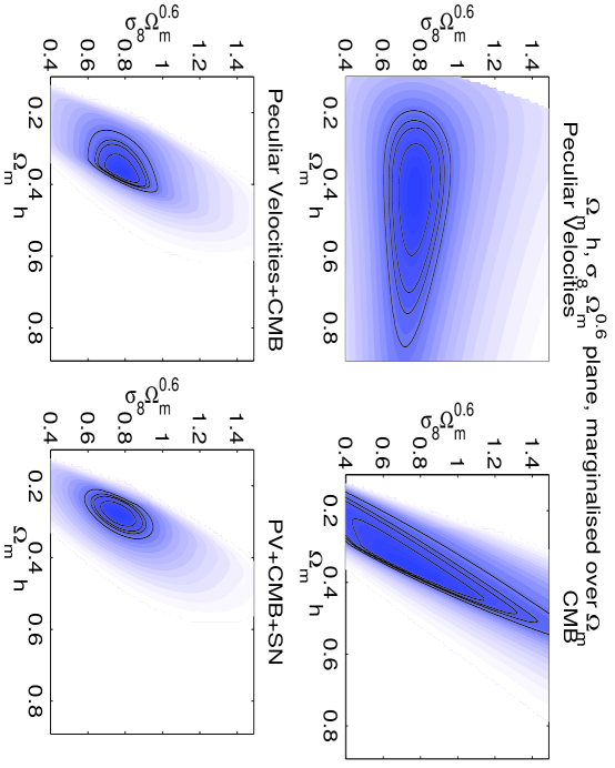
Figure 5.: Joint analysis of peculiar velocities with 2-D contours in the plane $\sigma_{8}\Omega_{m}^{0.6}$ (which controls the amplitude of the velocity field) and $\Omega_{m}h$ (which controls the shape of a CDM power-spectrum). The contours are shown for the peculiar velocities (PV), and the CMB independently and for the combination PV+CMB and PV+CMB+SN. We see that combining the sets helps significantly to constrain the parameters (from Bridle et al. 2000).

Several groups (e.g. Eisenstein, Hu & Tegmark 1998; Webster et al. 1998; Gawiser & Silk 1998; Bridle et al. 1999) have recently estimated cosmological parameters by joint analysis of data sets (e.g. CMB, SN, redshift surveys, cluster abundance and peculiar velocities) in the framework of FRW cosmology. The idea is the the cosmological parameters can be better estimated due to the complementary nature of the different probes.

While this approach is promising and we will see more of it in the next generation of galaxy and CMB surveys (2dF/SDSS/MAP/Planck) it is worth emphasizing a ‘health warning’ on this approach. First, the choice of parameters space is arbitrary and in the Bayesian framework there is freedom in choosing a prior for the model. Second, the ‘topology’ of the parameter space is only helpful when ‘ridges’ of 2 likelihood ‘mountains’ cross each other (e.g. as in the case of the CMB and the SN). It is more problematic if the joint maximum ends up in a ’valley’. Finally, there is the uncertainty that a sample does not represent a typical patch of the FRW Universe to yield reliable global cosmological parameters.

Webster et al. (1998) combined results from a range of CMB experiments, with a likelihood analysis of the IRAS 1.2Jy survey, performed in spherical harmonics. This method expresses the effects of the underlying mass distribution on both the CMB potential fluctuations and the IRAS redshift distortion. This breaks the degeneracy e.g. between $\Omega_{m}$ and the bias parameter. The family of CDM models analysed corresponds to a spatially-flat Universe with with an initially scale-invariant spectrum and a cosmological constant $\lambda$. Free parameters in the joint model are the mass density due to all matter ($\Omega_{m}$), Hubble’s parameter ($h=H_{0}/100$ km/sec), IRAS light-to-mass bias ($b_{iras}$) and the variance in the mass density field measured in an $8h^{-1}$ Mpc radius sphere ($\sigma_{8}$). For fixed baryon density $\Omega_{b}=0.02/h^{2}$ the joint optimum lies at $\Omega_{m}=1-\lambda=0.41\pm{0.13}$, $h=0.52\pm{0.10}$, $\sigma_{8}=0.63\pm{0.15}$, $b_{iras}=1.28\pm{0.40}$ (marginalised 1-sigma error bars). For these values of $\Omega_{m},\lambda$ and $H_{0}$ the age of the Universe is $\sim 16.6$ Gyr.

The above parameters correspond to the combination of parameters $\Omega_{m}^{0.6}\sigma_{8}=0.4\pm 0.2$. This is quite in agreement from results form cluster abundance (Eke et al. 1998), $\Omega_{m}^{0.5}\sigma_{8}=0.5\pm 0.1$. By combining the abundance of clusters with the CMB and IRAS Bridle et al. (1999) found $\Omega_{m}=1-\lambda=0.36$, $h=0.54$, $\sigma_{8}=0.74$, and $b_{iras}=1.08$ (with error bars similar to those above).

On the other hand, results from peculiar velocities yield higher values (Zehavi & Dekel 1999 and in these proceedings), $\Omega_{m}^{0.6}\sigma_{8}=0.8\pm 0.1$. By combining the peculiar velocities (from the SFI sample) with cluster abundance and SN Ia one obtains overlapping likelihoods at the level of $2-sigma$ (Bridle et al. 2000). The best fit parameters are $\Omega_{m}=1-\lambda=0.52$, $h=0.57$, and $\sigma_{8}=1.10$. As the $\Omega_{m}$ from peculiar velocities is higher than that from the other probes, the joint value is higher than above.

The 3-D likelihoods are shown in Zehavi& Dekel in this volume. We show in the Figure 5 the 2-D contours in the plane $\sigma_{8}\Omega_{m}^{0.6}$ (which controls the amplitude of the velocity field) and $\Omega_{m}h$ (which controls the shape of a CDM power-spectrum). The contours are shown for the peculiar velocities (PV), and the CMB independently and for the combination PV+CMB and PV+CMB+SN. We see that combining the sets helps significantly to constrain the parameters.

7. Discussion

Analysis of the CMB, the XRB, radio sources and the Lyman-$\alpha$ which probe scales of $\sim 100-1000\,h^{-1}\,{\rm Mpc}$ strongly support the Cosmological Principle of homogeneity and isotropy. They rule out a pure fractal model. However, there is a need for more realistic inhomogeneous models for the small scales. This is in particular important for understanding the validity of cosmological parameters obtained within the standard FRW cosmology.

Joint analyses of the CMB, IRAS, SN, cluster abundance and peculiar velocities suggests $\Omega_{m}=1-\lambda\approx 0.3-0.5$.

With the dramatic increase of data, we should soon be able to map the fluctuations with scale and epoch, and to analyze jointly LSS (2dF, SDSS) and CMB (MAP, Planck) data, taking into account generalized forms of biasing.

Acknowledgments.

I thank my collaborators for their contribution to the work presented here.

References

Baleisis, A., Lahav, O., Loan, A.J. & Wall, J.V. 1998, MNRAS, 297, 545

Baugh C.M. & Efstathiou G. 1994, MNRAS , 267, 323

Boldt, E. A. 1987, Phys. Reports, 146, 215

Bridle, S.L., Eke, V.R., Lahav, O., Lasenby, A.N., Hobson, M.P., Cole, S., Frenk, C.S., & Henry, J.P. 1999, MNRAS, in press, astro-ph/9903472

Bridle, S.L., Zehavi, I., Dekel, A., Lahav, O., Hobson, M.P. & Lasenby, A.N., 2000, in preparation

Buchert T & Ehlers, J. 1997, A&A, 320, 1

Célérier, M.N. 1999, submitted to A&A (astro-ph/9907206)

Cress C.M., Helfand D.J., Becker R.H., Gregg. M.D. & White, R.L. 1996, ApJ, 473, 7

Davis, M. 1997, Critical Dialogues in Cosmology, World Scientific, ed. N. Turok, pg. 13.

Dekel, A. et al., 1999, ApJ, in press (astro-ph/9812197)

Dyer, C.C. & Roeder, R.C. 1973, ApJ, 180, L31

Ehlers, J., Geren, P & Sachs, R.K. 1968, J Math Phys, 9(9), 1344, 1968

Eisenstein, D.J., Hu, W. & Tegmark, M. 1998 (astro-ph/9807130)

Eke, V.R., Cole, S., Frenk, C.S. & Henry, J.P. 1998, MNRAS, 298, 1145

Fabian, A. C. & Barcons, X. 1992, ARAA, 30, 429

Gawiser, E. & Silk, J., 1998, Science, 280, 1405

Giovanelli, R. et al. 1999, submitted to ApJ (astro-ph/9906362)

Hoffman, Y., 1999, in Evolution of Large Scale Structure, MPA/ESO Conference, August 1997, eds. A. Banday & R. Sheth.

Holz, D.E. & Wald, R.M. 1998, Phys Rev D, 58, 063501

Joyce, M., Montuori, M., Sylos-Labini F. & Pietronero, L., 1999, A&A, 344, 387

Kantowski, R. 1998, ApJ, 507, 483

Krasinski, A. 1997, Inhomogeneous Cosmological Models, Cambridge University Press, Cambridge

Lahav O., Piran T. & Treyer M.A. 1997, MNRAS, 284, 499

Lahav, O., Santiago, B.X., Webster, A.M., Strauss, M.A., Davis, M., Dressler, A. & Huchra, J.P. 1999, MNRAS, in press

Lilje, P.B., Yahil, A. & Jones, B.J.T. 1986, ApJ, 307, 91

Maartens, R., Ellis, G. F. R. & Stoeger, W. R. 1996, A&A , 309, L7

Magliocchetti, M., Maddox, S.J., Lahav, O.& Wall, J.V. 1998, MNRAS, 300, 257

Metcalf, R. B. , Silk, J. 1999, ApJ L, 519, L1

Nusser, A. & Lahav, O. 1999, submitted to MNRAS (astro-ph/991017)

Peebles, P. J. E. 1993, Principles of Physical Cosmology, Princeton University Press, Princeton.

Perlmutter et al. 1999, ApJ, 517, 565

Pietronero, L., Montuori M., & Sylos-Labini, F. 1997, in Critical Dialogues in Cosmology, World Scientific, ed. N. Turok, pg. 24

Rudnicki, K. 1995, The cosmological principles, Jagiellonian University, Krakow 1995

Scaramella, R. et al. 1998, A&A, 334, 404

Scharf, C.A., Jahoda, K., Treyer, M., Lahav, O., Boldt, E. & Piran, T., et al., 1999, submitted to ApJ (astro-ph/9908187)

Schmoldt, I. et al. 1999, MNRAS, 304, 893

Strauss M.A. et al., 1992, ApJ, 397, 395

Tomita, K. 1999 (astro-ph/9906027)

Treyer, M., Scharf, C., Lahav, O., Jahoda, K., Boldt, E. & Piran, T. 1998, ApJ, 509, 531

Webster, M.A., Lahav, O., & Fisher, K.B. 1998, MNRAS, 287, 425

Webster, M., Hobson, M.P., Lasenby, A.N., Lahav, O., Rocha, G. & Bridle, S. 1998, ApJ, 509, L65

Wu, K.K.S., Lahav, O. & Rees, M.J. 1998, Nature, 397, 225

Zehavi,I & Dekel, A. 1999, Nature, 401, 252

Zehavi, I, Riess, A.G., Kirshner, R.P. & Dekel, A. 1998, ApJ, 503, 483

Zeldovich, Ya, B. 1964, Soviet Astron, 8, 13