Microwave background anisotropies due to non-linear structures in open and $\Lambda$ universes

Abstract

A new method arising from a gauge-theoretic approach to general relativity is applied to the formation of clusters in an expanding universe. The three cosmological models ($\Omega_{0}$=1, $\Omega_{\Lambda}$=0), ($\Omega_{0}$=0.3, $\Omega_{\Lambda}$=0.7), ($\Omega_{0}$=0.3, $\Omega_{\Lambda}$=0) are considered, which extends our previous application (Lasenby et al. 1999, Dabrowski et al. 1999). A simple initial velocity and density perturbation of finite extent is imposed at the epoch $z=1000$ and we investigate the subsequent evolution of the density and velocity fields for clusters observed at redshifts $z=1$, $z=2$ and $z=3$. Photon geodesics and redshifts are also calculated so that the Cosmic Microwave Background (CMB) anisotropies due to collapsing clusters can be estimated. We find that the central CMB temperature decrement is slightly stronger and extends to larger angular scales in the non-zero $\Omega_{\Lambda}$ case. This effect is strongly enhanced in the open case. Gravitational lensing effects are also considered and we apply our model to the reported microwave decrement observed towards the quasar pair PC 1643+4631 A&B.

1 Secondary Gravitational Effect

Rees and Sciama (1968) suggested that the presence of an evolving structure on the line of sight of a Cosmic Microwave Background (CMB) photon could significantly affect its observed temperature. This secondary gravitational effect is often described in terms of the potential well experienced by the CMB photon. For example, the potential well of a collapsing cluster becomes deeper over time so that the CMB photon has to climb out of a well deeper than that into which it fell, suffering a net loss of energy. As suggested in Rees and Sciama (1968) there is however a competing effect due to the extra time delay encountered by the photon. The overall effect can therefore be of either sign. The photon accumulates a redshift along its geodesic, resulting in a net temperature perturbation. In the weak-field approximation we have (see Martínez-González, Sanz & Silk 1990)

$$\frac{\Delta T}{T}=-\frac{2}{c^{2}}\int\frac{\partial\Phi}{\partial t}dt,$$ (1)

where $\Phi$ is the gravitational potential of the perturbation and $t$ is the cosmic time. A rough estimate of an upper limit to this effect can be estimated by assuming that the potential well varies from $\Phi=0$ to $\Phi=\Phi_{c}$ during the time that the photon traverses it, where $\Phi_{c}$ is the gravitational potential of a rich Abell cluster. In this case, we have

$$\frac{\Delta T}{T}<-\frac{2}{c^{2}}\Phi_{c}.$$ (2)

The potential of the cluster can be related to the velocity dispersion $\sigma$ through $\sigma^{2}=GM/R=\Phi_{c}$, where $M$ and $R$ are the mass and radius of the cluster. Assuming $\sigma=1000$ km s^-1 gives

$$\frac{\Delta T}{T}<-2.2\times 10^{-5}.$$ (3)

In most cases, this anisotropy should therefore be small compared with other secondary anisotropies caused by the interaction of CMB photons with non-linear structures, such as the thermal Sunyaev-Zel’dovich (SZ) effect. However, equation (1) is only valid in the linear regime and a fully relativistic treatment in the non-linear regime is necessary to estimate accurately the Rees-Sciama effect.

Several methods have been used to model the formation of galaxy clusters in an expanding universe. The modelling of arbitrary perturbations in a fully general relativistic manner has not proved possible due to the complexity of the calculations involved. The most popular method has been the linearised approach (equation 1), allowing the modelling of arbitrarily shaped inhomogeneities (Martínez-González & Sanz 1990; Martínez-González et al. 1990; Chodorowski 1991). This method has been particularly used for Great Attractor-like structures located at redshifts as high as $z=5.9$, where less strong non-linear effects are expected (Sáez, Arnau & Fullana 1993, 1995; Arnau, Fullana & Sáez 1994; Fullana, Sáez & Arnau 1994).

In this paper we are interesting in modelling rich galaxy clusters which are often ellipsoid or even quasi spherical (e.g. Coma cluster). This leads to spherical symmetry as a natural approximation, which allows a general relativistic derivation. The earliest attempts of modelling are of the Swiss Cheese type, where the collapsing Friedmann-Robertson-Walker (FRW) region is compensated for by a surrounding region of vacuum matched onto the expanding FRW universe (Rees & Sciama 1968; Nottale 1982; Nottale 1984). In these models, analytic calculations can be performed in the fully non-linear regime and the observer can be located in the external, unperturbed universe. However, the matter distribution is unrealistic.

More recent models have used the Tolman-Bondi solution for a pressureless, spherically symmetric matter distribution to provide a more realistic density perturbation (Panek 1992; Quilis, Ibáñez & Sáez 1995; Quilis and Sáez 1998). These, however, are rarely compensated and comoving observers are not in a region modelled by a homogeneous FRW metric, which adds difficulty in estimating the temperature anisotropy.

Finally, a new model arising from a gauge-theoretic approach to gravity was proposed by Lasenby et al. (1999). This method employs a gauge, mainly characterised by a unique global time coordinate, which reduces the equations to an essentially Newtonian form. The model avoids the problem of streamline crossing, while keeping the density profile compensated and realistic. Furthermore, the perturbation is of finite size, allowing the observer to be placed in a non-perturbed region.

In this paper we extend this new theoretical approach to the case of a non-zero cosmological constant $\Lambda$ and to the case of open cosmologies. The non-zero $\Lambda$ model is of particular interest since recent observations of high redshift Type Ia supernovae are inconsistent with $\Lambda=0$ flat or open cosmologies, suggesting that our universe may be accelerating (Perlmutter et al. 1997, 1999). When the Type Ia supernovae results are combined with observations of the CMB, an approximately flat FRW cosmological model is suggested with $\Omega_{0}\approx 0.3$ and $\Omega_{\Lambda}\approx 0.7$ (Efstathiou et al. 1999). $\Omega_{0}$ is the mass density parameter at the present epoch and $\Omega_{\Lambda}=\Lambda/3H_{0}^{2}$, where $H_{0}$ is the Hubble constant at the present time.

2 Assumptions

Three cosmological models are considered here: The Einstein de Sitter (EdS), Flat-$\Lambda$ and Open models, corresponding to ($\Omega_{0}$=1, $\Omega_{\Lambda}$=0), ($\Omega_{0}$=0.3, $\Omega_{\Lambda}$=0.7), and ($\Omega_{0}$=0.3, $\Omega_{\Lambda}$=0) respectively. Results will be quoted using the reduced Hubble parameter $h(t)$, which is equal to $H(t)$ expressed in units of $100$ km s^-1Mpc^-1. Furthermore, quantities evaluated at the present time $t=t_{0}$ will be written simply with a zero subscript, e.g., $h(t_{0})=h_{0}$. Throughout this work we take $t_{i}$, the time at which the initial perturbation is applied, to represent the epoch $z=1000$. We employ natural units $G=c=\hbar=1$, unless stated otherwise.

Throughout this paper, we assume that the cosmological fluid as well as the evolving non-linear structure are pressureless. Quilis et al. (1995) included a hot gas component in their model and found that the pressure effects are in fact negligible and that the collapse is well approximated by the pressureless assumption.

As mentioned above, the perturbation is assumed to be spherically symmetric which, combined with the pressureless assumption, leads to the unrealistic situation where the structure collapses to form a singularity. As a result, the estimates of CMB anisotropies given in this work should be regarded as upper limits. However, the initial perturbations are chosen so that the CMB photon traverses the cluster before it becomes singular. Throughout this paper, the maximum baryonic density experienced by the photon at the centre of the non-linear structure is set to $10^{4}h_{0}^{1/2}~{}{\rm protons~{}m^{-3}}$. Furthermore the clusters considered in this work are located at high redshifts ($z=1$, $z=2$ and $z=3$) and should therefore still be in the process of formation. In these cases the large infalling motions predicted by the spherically symmetric pressureless assumptions may be less unrealistic.

We further assume that, at all times, the baryon component contributes $10h_{0}^{-3/2}$ per cent of the total mass, the remainder being dark matter. The $h$-dependence chosen here ensures that the total gravitational mass scales as $h_{0}^{-1}$, as expected within the isothermal sphere approximation (e.g. Peebles 1993). In this case the total density follows the power law form $\rho\propto r^{-2}$ and the baryon mass alone scales as $h_{0}^{-5/2}$.

3 Fluid Dynamics

This paper follows the theoretical approach of Lasenby et al. (1999) and Lasenby, Doran & Gull (1998) where exact and fully relativistic derivations are given using a new gauge-theoretic approach to gravity. The resulting field equations are remarkably straightforward and are here presented as if derived from classical first principles (see Lasenby et al. (1997) for rigorous calculations).

The forming cluster and the external universe are both described by the same dynamical equations, the centre of the cluster being at the origin of the spherical coordinates ($r$, $\theta$, $\phi$). Since we are only concerned with spherically symmetric systems, we choose hereafter $\theta=\pi/2$ without loss of generality. The symbol $t$ is used for the dynamical time.

The two scalar quantities needed to describe the fluid dynamics are the density $\rho(t,r)$ and the radial velocity

$$u(t,r)=\frac{{\rm d}r}{{\rm d}t}$$ (4)

along matter geodesics. The total gravitational mass $M(t,r)$ contained within a sphere of radius r is defined by

$$\left(\frac{\partial M}{\partial r}\right)_{t}=4\pi r^{2}\rho,$$ (5)

or

$$M(t,r)=\int^{r}_{0}4\pi r^{\prime 2}\rho(t,r^{\prime})dr^{\prime}.$$ (6)

The mass of fluid flowing through a sphere of radius $r$ per unit time is given by

$$\left(\frac{\partial M}{\partial t}\right)_{r}=-4\pi r^{2}\rho u.$$ (7)

One can define the streamline derivative (i.e. co-moving with the fluid) as

$$\frac{{\rm d}}{{\rm d}l}\equiv\frac{\partial}{\partial t}+u\frac{\partial}{\partial r}.$$ (8)

We can see from (5) and (7) that the total gravitational mass enclosed is conserved along the fluid streamlines,

$$\frac{{\rm d}M}{{\rm d}l}=0,$$ (9)

which forbids the possibility of streamline crossing.

3.1 Equation of Continuity

By equating the total mass of fluid flowing out of a given volume per unit time to the decrease per unit time of fluid in the same volume, one obtains the standard equation of continuity

$$\frac{{\rm d}\rho}{{\rm d}l}=\frac{\partial\rho}{\partial t}+u\frac{\partial\rho}{\partial r}=-\left(\frac{2u}{r}+H\right)\rho,$$ (10)

where

$$H(t,r)\equiv\frac{\partial u(t,r)}{\partial r}.$$ (11)

3.2 Euler’s Equation

Newton’s second law applied on a fluid particle gives the usual Euler’s equation

$$\frac{\partial u}{\partial t}+u\frac{\partial u}{\partial r}=F(t,r),$$ (12)

where $F$ is the total force applied on the particle. $F$ includes the radial gravitational force $F_{g}=-M/r^{2}$ as well as the repulsive force $F_{\Lambda}$ proportional to $r$ due to the cosmological constant $\Lambda$. To agree with the usual convention we set the constant of proportionality to $\Lambda/3$ so that $F_{\Lambda}=(\Lambda/3)r$. Finally equation (12) reads

$$\frac{{\rm d}u}{{\rm d}l}=\frac{\partial u}{\partial t}+u\frac{\partial u}{\partial r}=-\frac{M}{r^{2}}+\frac{\Lambda}{3}r.$$ (13)

3.3 Bernoulli’s Equation

Multiplying Euler’s equation (13) by $u$ and integrating along the streamline ${\rm d}l$, gives

$$\frac{1}{2}u^{2}-\left(\frac{M}{r}+\frac{\Lambda}{6}r^{2}\right)=E(t,r),$$ (14)

where the constant of integration $E(t,r)$ is constant along the fluid streamlines, i.e.

$$\frac{{\rm d}E}{{\rm d}l}=0.$$ (15)

In equation (14), $u^{2}/2$ can be regarded as the kinetic energy of a fluid particle, while $-M/r-(\Lambda/6)r^{2}$ can be thought of as its potential energy composed of the usual gravitational potential and a potential proportional to $r^{2}$ due to the presence of a cosmological constant. $E(t,r)$ can therefore be associated with the total energy of a fluid shell. If $E<0$ the shell will eventually collapse at the origin while if $E>0$ the shell will remain in expansion. In other words, equation (14) can be regarded as a generalised Friedman equation for which each fluid shell is allowed a different constant $E$.

3.4 Newtonian Gauge

The physical significance of the above set of equations is remarkably straightforward yet, as shown in Lasenby et al. (1998), they are fully consistent with general relativity. This is because the degrees of freedom offered by the gauge theoretic approach have been carefully chosen so that the resulting equations look Newtonian. In particular the gauge fields have been fixed so that the coordinate $r$ is a measurable distance scale related to the strength of the tidal force, and the coordinate $t$ is a measure of the proper time $\tau$ for all observers comoving with the fluid, therefore ${\rm d}t$ = ${\rm d}l$ = ${\rm d}\tau$, $l$ being the affine parameter of the streamlines (equation 8). Therefore this gauge choice enables us to recover a global “Newtonian” time on which all observers can agree. Lasenby et al. (1998) have named this gauge the Newtonian Gauge. The associated line element is given by

$${\rm d}s^{2} = \left(1-\frac{u^{2}}{2E+1}\right){\rm d}r^{2}+\frac{2u}{2E+1}{\rm d}t{\rm d}r-\frac{1}{2E+1}{\rm d}r^{2}$$ (16)

$$-r^{2}\left({\rm d}\theta^{2}+\sin^{2}\theta{\rm d}\phi^{2}\right).$$

Similar analytic solutions have been found by Tolman (1934) and Bondi (1947), however their use of $M(r)$ as the radial coordinate rather than $r$ has the disadvantage of hiding the physical meaning of the field equation and complicates the choice of initial conditions.

In homogeneous regions the fluid behaves as for standard cosmologies and the density $\rho$ is a function of time only, so we have

$$\bar{M}(t,r)=\frac{4\pi}{3}r^{3}\bar{\rho}(t),$$ (17)

where the overbar denotes quantities in the external homogeneous region. Here, equations (9), (10) and (13) lead to

$$\frac{{\rm d}\bar{\rho}}{{\rm d}t}=-3\bar{H}\bar{\rho}(t),$$ (18)

$$\bar{H}(t)=\frac{\bar{u}}{r},$$ (19)

and

$$\frac{{\rm d}\bar{H}}{{\rm d}t}+\bar{H}^{2}=-\frac{4\pi}{3}\bar{\rho}+\frac{\Lambda}{3}.$$ (20)

It is clear from those standard results that we can identify $\bar{H}$ as the Hubble constant, and that the time parameter $t$ of the Newtonian gauge agrees with the cosmic time in homogeneous regions of our model. We also have

$$\frac{8\pi}{3}\bar{\rho}(t)=\bar{H}(t)^{2}\Omega(t),$$ (21)

for the EdS and Open models and

$$\frac{8\pi}{3}\bar{\rho}(t)=\bar{H}^{2}(t)-\frac{1}{3}\Lambda,$$ (22)

for the Flat-$\Lambda$ model.

3.5 Streamline Equations

In general, the solution to equation (14) can be expressed in terms of elliptic integrals. We choose here to integrate numerically this equation using the following system of two first order ordinary differential equations composed of (4) and Euler’s equation:

$$\frac{{\rm d}r}{{\rm d}t} = u$$

$$\frac{{\rm d}u}{{\rm d}t} = -\frac{M(r_{i})}{r^{2}}+\frac{\Lambda}{3}r,$$ (23)

where $r_{i}$ is the fluid particle radius on a given streamline, at an initial time $t_{i}$. This system allows us to compute the position $r$ of the fluid particle as well as its velocity $u$ at a later time $t$. We note that, in this manner, the change from positive $u$ to negative $u$ is automatically evaluated in the case of closed streamlines. The fluid density $\rho(t,r)$ and velocity gradient $H(t,r)$ are calculated by differentiating numerically equations (5) and (11).

However, equation (14) has analytical solutions in two particular cases. (i) For $\Lambda=0$, which corresponds to the standard Friedman models. This case is treated in detail in Lasenby et al. (1999). (ii) For $E=0$, where the solution is given by the following streamline equation

$$t=t_{i} + \frac{1}{\sqrt{3\Lambda}}{\rm arccosh}\left(\frac{\Lambda}{3M(r_{i})}r^{3}+1\right)$$ (24)

$$- \frac{1}{\sqrt{3\Lambda}}{\rm arccosh}\left(\frac{\Lambda}{3M(r_{i})}r_{i}^{3}+1\right).$$

In this case, the value of the velocity along the streamline is given by (14) itself:

$$u=\sqrt{\frac{2M(r_{i})}{r}+\frac{\Lambda}{3}r^{2}}.$$ (25)

We note that here $u$ is always positive since $E=0$. Following Lasenby et al. (1999), the density is given by

$$\rho(t,r)=\left(\frac{\partial r_{i}}{\partial r}\right)_{t}\frac{r_{i}^{2}}{r^{2}}\rho(r_{i}),$$ (26)

where

$$\left(\frac{\partial r_{i}}{\partial r}\right)_{t}^{-1}=\frac{1}{Mr^{\frac{1}{2}}\sqrt{\Lambda r_{i}^{3}+6M}}\Big{[}Mr_{i}^{\frac{1}{2}}\sqrt{\Lambda r^{3}+6M}+$$

$$\frac{4\pi}{3}r_{i}^{2}\rho(r_{i})\left(r^{\frac{3}{2}}\sqrt{\Lambda r_{i}^{3}+6M}-r_{i}^{\frac{3}{2}}\sqrt{\Lambda r^{3}+6M}\right)\Big{]}.$$ (27)

The velocity gradient is found by differentiating equation (14), which leads to

$$\frac{\partial u}{\partial r}=-\frac{M}{r^{2}u}+\Lambda\frac{r}{3u}+\frac{1}{u}\left(\frac{\partial r_{i}}{\partial r}\right)_{t}\left[\frac{1}{r}\frac{{\rm d}M}{{\rm d}r_{i}}+\frac{{\rm d}E}{{\rm d}r_{i}}\right].$$ (28)

4 Cluster Formation Model

The fluid equations given above control the evolution of the external homogeneous cosmology as well as the formation of the central cluster. The initial perturbation is applied at an early time $t_{i}$ that we choose here to represent the epoch $z=10^{3}$. The perturbation is of finite extent and we therefore need to fix initial conditions so that standard cosmology is satisfied outside a given radius $R_{i}$. Here we will use a family of simple four-parameter models based on polynomial perturbations in the density and velocity fields, as described in detail in Lasenby et al. (1999) and Dabrowski et al. (1999). The parameters are (i) the width of the perturbation $R_{i}$; (ii) the velocity gradient at the origin $H(t_{i},0)$; (iii) the degree of the polynomial describing the perturbation, so that at $r=R_{i}$, the velocity and its first $m$ derivatives match the external values; (iv) the external velocity gradient $\bar{H}(t_{i})$ equal to the Hubble constant at the time $t_{i}$. As a typical value, we assume in this paper $m=3$.

4.1 Linearised Equations

The perturbation responsible for the formation of clusters of galaxies is assumed to have grown from primordial fluctuations in the very early universe. At the epoch $z=10^{3}$, the fluid dynamics should still be well described by considering evolution in the linear regime.

We introduce the linearised variables

$$\delta u \equiv u-r\bar{H}(t)$$

$$\delta\rho \equiv \rho-\bar{\rho}(t)$$ (29)

$$\delta M \equiv \int^{r}_{0}4\pi s^{2}\delta\rho(t,s)ds\,,$$

where the overbarred quantities denote background homogeneous universe values. Differentiating equation (4.1) gives

$${\frac{{\rm d}\delta u}{{\rm d}t}}=-\frac{\delta M}{r^{2}}-\bar{H}\delta u\,,$$ (30)

as in the $\Lambda=0$ case (see Lasenby et al. 1999). Differentiating again and ignoring second order terms yields

$${\frac{{\rm d}}{{\rm d}t}}\left({\frac{{\rm d}\delta u}{{\rm d}t}}\right)+3\bar{H}{\frac{{\rm d}\delta u}{{\rm d}t}}-\bar{H}^{2}\delta u+\Lambda\delta u=0\,,$$ (31)

where the background universe is assumed to be spatially flat ($E=0$). By parameterising $\delta u$ in terms of streamline starting point, $r_{i}$ and cosmic time, $t$, the streamline derivatives become derivatives with respect to $t$:

$$\delta\ddot{u}+3\bar{H}\delta\dot{u}-(\bar{H}^{2}-\Lambda)\delta u=0\,,$$ (32)

where the overdot denotes derivatives with respect to $t$. In the limit of small $t$ and $\Lambda$

$$\bar{H}\approx\frac{2}{3t}+\frac{\Lambda}{6}t,$$ (33)

and $\delta u$ goes as

$$\delta u=A{t^{-4/3}}+Bt^{1/3}+O(t^{2/3})\,.$$ (34)

Assuming that we are in an epoch where the decaying mode $t^{-4/3}$ can be ignored but sufficiently early that the $t^{2/3}$ term is not yet significant, then

$${\frac{{\rm d}\delta u}{{\rm d}t}}=\frac{1}{2}\bar{H}\delta u\,.$$ (35)

Alternatively, it can be said that at early enough times, $\bar{H}^{2}\gg\Lambda$ and so the $\Lambda$ term may be ignored in equation (32). Thus using equation (30) we have

$$\frac{3}{2}\bar{H}\delta u=-\frac{\delta M}{r^{2}}\,,$$ (36)

or expressed in terms of the perturbed and un-perturbed quantities

$$u=r\bar{H}-\frac{2M}{3\bar{H}r^{2}}+\frac{r}{3\bar{H}}\frac{8\pi}{3}\bar{\rho}.$$ (37)

Substituting $8\pi\bar{\rho}/3$ with values of equations (21) and (22) gives an extra condition on the initial data

$$u(t_{i},r)=\frac{2r}{3\bar{H}}\left(\frac{3+\Omega_{0}}{2}\bar{H}^{2}-\frac{M}{r^{3}}\right),$$ (38)

for the EdS and Open models and

$$u(t_{i},r)=\frac{2r}{3\bar{H}}\left(2\bar{H}^{2}-\frac{M}{r^{3}}-\frac{1}{6}\Lambda\right),$$ (39)

for the Flat-$\Lambda$ model. The initial density perturbation can now be derived from the initial velocity field as follows: Differentiating (38) and (39) with respect to $r$ gives

$$\rho(t_{i},r)=\frac{3\bar{H}}{8\pi}\left[\left(3+\Omega_{0}\right)\bar{H}-\frac{2u}{r}-\left(\frac{\partial u}{\partial r}\right)_{t_{i}}\right],$$ (40)

for the EdS and Open cosmologies, and

$$\rho(t_{i},r)=\frac{3\bar{H}}{8\pi}\left[4\bar{H}-\frac{2u}{r}-\left(\frac{\partial u}{\partial r}\right)_{t_{i}}-\frac{1}{3\bar{H}}\Lambda\right],$$ (41)

for the Flat-$\Lambda$ case.

4.2 Initial Conditions

At the time $t_{i}$, the initial conditions are defined completely by the 4 parameter velocity profile while the corresponding initial density profile is given by equation (40) or (41). The external universe $\bar{H}(t_{i})$ is fully defined by the desired cosmology (i.e. $\Omega_{0}$, $\Omega_{\Lambda}$ and $h_{0}$). We have for the EdS and Open models

$$\bar{H}(t_{i})=H_{0}(1+z_{i})\sqrt{1+\Omega_{0}z_{i}},$$ (42)

and for the Flat-$\Lambda$ cosmology

$$\bar{H}(t_{i})=\sqrt{\left(1+z_{i}\right)^{3}\left(H_{0}^{2}-\frac{1}{3}\Lambda\right)+\frac{1}{3}\Lambda}.$$ (43)

The two remaining parameters $R_{i}$ and $H(t_{i},0)$ are fixed such that the resulting cluster is similar to those observed today, using the following characteristics: the redshift of the cluster $z_{c}$, its core radius $R_{c}$ (where $R_{c}$ is defined as the radius at which the cluster density falls to one-half its maximum value) and its central baryonic density $\rho_{c}$. Because we are interested in modelling rich clusters, the core radius is fixed to $R_{c}=0.23h_{0}^{-1}$ Mpc and the central density is taken to be $\rho_{c}=10^{4}h_{0}^{1/2}$ ${\rm p~{}m}^{-3}$. The $h$-dependences of $R_{c}$ and $\rho_{c}$ are chosen so that the cluster’s observed angular size and X-ray flux are independent of $h_{0}$ (Jones & Forman 1984; Peebles 1993). Figs. 1 and 2 show the initial velocity and density profiles in the Open , Flat-$\Lambda$ and EdS models. In all three cases, the resulting cluster observed at $z_{c}=1$ satisfies the same properties $R_{c}=0.23h_{0}^{-1}$ Mpc and $\rho_{c}=10^{4}h_{0}^{1/2}$ ${\rm p~{}m}^{-3}$.

Figure 1: Initial relative velocity $u(t_{i},r)-\bar{H}(ti)r$ where $t_{i}$ represents the epoch $z=10^{3}$. The solid, dashed and dotted lines are for the Open , Flat-$\Lambda$ ($\Omega_{\Lambda}=0.7$) and EdS models respectively.

Figure 2: As in Fig. 1, but for the initial density contrast $\rho(t_{i},r)/\bar{\rho}(t_{i})$.

We note that low-$\Omega_{0}$ models require larger and deeper perturbation. This can be explained as follows: The equation equivalent to (32) but for the density perturbation evolution is given by

$$\ddot{\delta}=4\pi\bar{\rho}\delta-2\bar{H}\dot{\delta},$$ (44)

where $\delta=\delta\rho/\bar{\rho}$. The first term of the right hand side governs the growth of the perturbation while the second can be regarded as a damping term due to the drag from the expansion of the universe. In the low density universe cases (Flat-$\Lambda$ and Open models), the growth term is smaller than in the critical density EdS model. Furthermore, $\bar{H}$ is larger in the Flat-$\Lambda$ and Open cosmologies (see equations 21 and 22), enhancing the damping term. Therefore it is to be expected that the initial perturbations in the case of the Flat-$\Lambda$ and Open models have to be larger than in the EdS case in order to give rise to similar structures at a later time. A more detailed study shows that in the Flat-$\Lambda$ model the growth suppression is less marked than for the Open model (see Peacock 1999). This explains why the initial perturbation of the Flat-$\Lambda$ case is less pronounced than for the Open case, as seen in Figs. 1 and 2.

4.3 Cluster Characteristics

As discussed in Section 2, the pressureless and spherically symmetric assumptions inevitably lead to non linear structures with large infall velocities, which would probably be realistic only for distant clusters still in the process of formation. Clusters observed at redshift $z=1$, $z=2$ and $z=3$ will be considered here and in the following sections.

The central density profile obtained at $z=1$ when applying the initial conditions of Section 4.2 is given in Fig. 3 up to the $1.5h_{0}^{-1}$ Mpc Abell radius, where the Open model is assumed.

Figure 3: The baryonic density of the cluster as a function of radius at the time corresponding to the redshift $z=1$. The dashed line is the best-fitting $\beta$-model up to $r=1.5h_{0}^{-1}$ Mpc. The Open model has been assumed here (see text).

We found that the central density profiles obtained in the context of the EdS and Flat-$\Lambda$ cosmologies are almost indistinguishable from that of the Open case. Furthermore, varying the redshift at which the cluster is observed from $z=1$ to $z=3$ does not affect the central density profile either. It is remarkable that by only fixing the desired central density $\rho_{c}$ and core radius $R_{c}$, the resulting density profile is almost identical in any cosmologies and at any redshift despite the significant difference between the initial perturbations, as seen in Figs. 1 and 2. However, it was found in Dabrowski et al. (1999) that the shape of the density profile is sensitive to the other free parameter of our model $m$, which is here set to $m=3$.

As discussed in detail in Dabrowski et al. (1999), the obtained density profile is well fitted by $\beta$-models

$$\rho(r)=\frac{\rho_{0}}{\left[1+\left(\frac{r}{R}\right)^{2}\right]^{\frac{3}{2}\beta}},$$ (45)

usually used to fit observed profiles and rotation curves. It was also found that density distributions such as those derived from N-body codes (Navarro Frenk & White 1996, 1997, hereafter NFW) give good agreement as regard the corresponding mass distribution of the cluster. However, the best least-square fit is obtained for a $\beta$-model with $\beta=2/3$. Indeed, as mentioned in Section 2 our model predicts density profiles $\rho\propto r^{-2}$ away from the origin which is more consistent with a $\beta=2/3$ model than with the NFW density profiles which behave like $r^{-3}$. Another difference between the density profiles obtained here and those of NFW is regarding their behaviour at the centre of the cluster. In this work the central density keeps a finite value while it diverges to infinity in the case of NFW density profiles.

The velocity distribution, as evolved at the time where the cluster is observed, is shown in Fig. 4 for $z=1$ and for the three EdS , Flat-$\Lambda$ and Open models.

Figure 4: The velocity distribution relative to the Hubble flow $u(t,r)-\bar{H}(t)r$ as a function of radius at the time corresponding to the redshift $z=1$. The solid, dashed and dotted lines are for the Open , Flat-$\Lambda$ and EdS cosmologies respectively.

As expected from an initial perturbation of finite extent, the velocity profile matches exactly that of the external homogeneous universe after a finite radius. This effect can be seen clearly on Fig. 4 where the velocity relative to the Hubble flow vanishes for $r>28h_{0}^{-1}$ Mpc in the EdS cosmology and for $r>55h_{0}^{-1}$ Mpc in the Flat-$\Lambda$ and Open cases. It is not surprising that this radius is roughly a factor of 2 smaller in the EdS model since the initial velocity and density perturbations were smaller in the same proportion, as seen in Figs. 1 and  2.

Other quantities of particular interest are the turnaround radius $R_{t}$, which is defined as the radius at which the fluid velocity changes from being radially inwards to radially outwards, and the ratio $\zeta$ of the cluster central density to that of the external universe. These characteristics, together with total gravitational masses contained within spheres of given radii, are summarised in Table 1 for clusters at redshifts $z=1$, $z=2$ and $z=3$ in the three EdS , Flat-$\Lambda$ and Open cosmologies. In all cases, the observed clusters have the same central density $\rho_{c}=10^{4}h_{0}^{1/2}{\rm~{}p~{}m^{-3}}$ and core radius $R_{c}=0.23h_{0}^{-1}$ Mpc.

Table 1: Cluster properties. $z$ denotes the redshift at which the cluster is observed (see text). $R_{t}$ is the turnaround radius quoted in $h_{0}^{-1}$ Mpc and $\zeta$ is the ratio of the central cluster density to that of the external Universe. $M_{1}$, $M_{1.5}$, $M_{2}$ and $M_{4}$ are total gravitational masses contained within spheres of radii $r=1$, $1.5$, $2$ and $4h_{0}^{-1}$ Mpc respectively. All masses are quoted in $10^{15}h_{0}^{-1}~{}{\rm M_{\odot}}$.

Model	$z$	$R_{t}$	$\zeta$	$M_{1}$	$M_{1.5}$	$M_{2}$	$M_{4}$
EdS	1	6.26	1122	1.05	1.80	2.65	6.70
Flat-$\Lambda$	1	10.74	3704	1.00	1.75	2.50	6.05
Open	1	8.70	3704	1.00	1.70	2.50	6.05
EdS	2	3.22	332.5	1.05	1.90	2.90	7.90
Flat-$\Lambda$	2	6.01	1097	1.00	1.85	2.65	6.75
Open	2	4.94	1097	1.00	1.85	2.65	6.75
EdS	3	1.97	140.3	1.10	2.10	3.15	9.50
Flat-$\Lambda$	3	3.82	463.0	1.05	1.90	2.80	7.50
Open	3	3.23	463.0	1.05	1.90	2.80	7.55

5 Photon Paths and Redshifts

In order to estimate the effect of non linear structure formation on the CMB we need to calculate the photon geodesics and redshifts in the context of the metric given in equation (16), as carried out in Lasenby et al. (1999). The photon motion is parametrised by the Newtonian time parameter $t$ discussed in Section 3.4. The path is defined by four quantities, the photon radius $r(t)$, position angle $\phi(t)$, 4-momentum direction $\chi(t)$ and frequency $\omega(t)$.

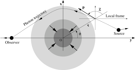
Figure 5: Geometrical arrangement defining the photon geodesic integration. The grey discs denote the spherically symmetric collapsing cluster which is located at the origin of the coordinate system. The photon is emitted from a source co-moving with the Hubble flow. The photon path is defined by the photon ($r$, $\phi$) position as well as the direction $\chi$ and frequency $\omega$ of its 4-momentum $p$.

As shown in Fig. 5, our model allows us to start a photon path at a given source position co-moving with the Hubble flow; integrate the geodesic equations through the homogeneous universe and through the collapsing cluster; and finally collect the photon at the observer position, co-moving with the Hubble flow as well. The calculation is identical in any spherically symmetric and pressure free cosmological model so that the set of four first order differential equation given in Lasenby et al. (1999) is still valid here.

6 Effect on the CMB

As discussed in Section 1, the presence of a time dependent potential on the line of sight will affect our observation of the CMB temperature. For the model considered here, Lasenby et al. (1999) found

$$\frac{\Delta T}{T}=\int_{t_{1}}^{t_{2}}\left(-{\frac{\partial\Delta}{\partial r}}\cos^{2}\chi-\frac{\Delta}{r}\sin^{2}\chi\right){\rm d}t,$$ (46)

where the integral is evaluated along the photon path. $\Delta$ is the fluid velocity relative to the Hubble flow

$$\Delta(t,r)=u(t,r)-r\bar{H}(t),$$ (47)

$t_{1}$ is time at the surface of last scattering and $t_{2}$ is the time at the observer. Numerical results are given in Table 2 for CMB photons that travel straight through the centre of collapsing clusters at $z=1$, $z=2$ and $z=3$.

Table 2: Estimates of the central temperature decrements $\Delta T/T$ in units of $10^{-5}$ for clusters at redshift $z=1$, $z=2$ and $z=3$. All clusters have the same central density $\rho_{c}=10^{4}h_{0}^{1/2}{\rm~{}p~{}m^{-3}}$ and core radius $R_{c}=0.23h_{0}^{-1}$ Mpc. Three cosmological models are considered.

Model	$\Delta T/T$, $z=1$	$\Delta T/T$, $z=2$	$\Delta T/T$, $z=3$
EdS	-0.64	-0.45	-0.32
Flat-$\Lambda$	-0.80	-0.64	-0.51
Open	-0.52	-0.43	-0.36

The EdS , and Open cosmological models considered here give roughly the same predictions for the central temperature decrement. We find however that the central anisotropy is slightly stronger in the Flat-$\Lambda$ case. When looking at the redshift dependence, Table. 2 shows that, for a given cluster central density and core radius, the further away the cluster is, the smaller the magnitude of the Rees-Sciama effect is. At earlier epochs, collapsing structures are less decoupled from the Hubble expansion and are therefore exposed to less strong non-linear effects, therefore it is not surprising that the effect gets dimmer.

         

Figure 6: Estimates of the angular distribution of the CMB anisotropy due to the presence of a collapsing cluster on the line of sight. From left to right, the three figures are for clusters at redshift $z=1$, $z=2$ and $z=3$ respectively. All clusters have the same central density $\rho_{c}=10^{4}h_{0}^{1/2}{\rm~{}p~{}m^{-3}}$ and core radius $R_{c}=0.23h_{0}^{-1}$ Mpc. The anisotropy is in units of $\Delta T/T$ as a function of the projected angle $\theta$ on the sky from the centre of the cluster. The solid, dashed and dotted lines are for the Open , Flat-$\Lambda$ and EdS cosmological models respectively. Note that the angular scale is different for each figure.

It is also useful to estimate the temperature anisotropy as a function of the projected angle $\theta$ on the sky from the centre of the cluster. Profiles of $\Delta T/T$ are given in Fig. 6 for the three EdS , Flat-$\Lambda$ and Open models and for clusters at $z=1$, $z=2$ and $z=3$. As noticed earlier, the magnitude of the effect gets smaller as the redshift of the cluster increases. Fig. 6 reveals that the angular distribution of the anisotropy is strongly dependent upon the cosmological model. In particular for the case where the cluster is located at $z=1$, the Open model estimate predicts a large and extended temperature increment on a scale of about one degree.

The fact that the temperature anisotropy can take positive as well as negative values is not surprising when looking at equation (46). As long as $\theta$ is not too small $(-\partial\Delta/\partial r)$ is negative, while $(-\Delta/r)$ is always positive, as seen in Fig.7. Typically, there are a negative and a positive contributions to the temperature anisotropy $\Delta T/T$ which are weighted by $\cos^{2}\chi$ and $\sin^{2}\chi$ respectively. For larger $\theta$, $\sin^{2}\chi$ is bigger and the positive exceeds the negative contribution.

Figure 7: Solid line: The integrand of equation (46), as a function of cosmic time $t$, along a photon path traversing a cluster located at $z=1$ with an angle of view $\theta=0.5$ degrees from the centre of the cluster. The time t=0 corresponds to the current epoch, and an Open model is assumed here. The central density of the cluster is $\rho_{c}=10^{4}h_{0}^{1/2}{\rm~{}p~{}m^{-3}}$ and its core radius $R_{c}=0.23h_{0}^{-1}$ Mpc. The corresponding temperature anisotropy $\Delta T/T$ is the area under the curve. The dashed and dotted lines are for $(-\partial\Delta/\partial r)$ and $(-\Delta/r)$ respectively.

The integrand of equation (46) is plotted in Fig. 7 along the path of a photon passing near the centre of a cluster located at $z=1$. The positive and negative contributions to the resulting $\Delta T/T$ are separated out. In this case, the overall perturbation is $\Delta T/T\sim+0.17\times 10^{-5}$.

In the case of the recently favoured Flat-$\Lambda$ cosmological model, it is interesting to note from Fig.6 that the temperature decrement is systematically stronger and extended to larger angles than in the other two models.

7 Gravitational Lensing and Time Delay

In this section we apply our model to the problem of the microwave decrement reported towards the quasar pair PC 1643+4631 A&B (Jones et al. 1997). This decrement is observed at 15 GHz and lies between a pair of quasars at redshifts $z=3.79$ and 3.83. The two quasars are separated by 198 arcsec. If the microwave decrement is assumed to be a thermal SZ effect caused by an intervening cluster, the minimum central temperature decrement is estimated to be $\Delta T/T$=$-2.1\times 10^{-4}$. However deep optical and infrared imaging carried with the WHT and the UKIRT (Saunders et al. 1997, Haynes et al. 1999) as well as ROSAT X-ray observations (Kneissl, Sunyaev & White 1998) suggest that any intervening cluster producing the temperature decrement should be located at a redshift as high as $z=3$. However, the presence of a cluster is supported by the remarkable similarity between the quasar spectra, suggesting gravitational lensing. Saunders et al. (1997) suggest that their $\sim 1$ per cent redshift difference can be explained in terms of quasar intrinsic evolution over a delay between the two lightpaths of $~{}\sim 10^{3}$ years. It was found in Dabrowski et al. (1999) that the time delays obtained in the EdS cosmology were too short. Here we propose to carry out a similar investigation but in the Flat-$\Lambda$ and Open cosmological models.

In this section, we assume $H_{0}=50~{}{\rm km~{}s^{-1}Mpc^{-1}}$; the maximum baryonic density along the photon path is still fixed to $10^{4}~{}{\rm p~{}m^{-3}}$; the total gravitational mass over baryonic mass ratio is 10. Following Dabrowski et al. (1999), we simplify the situation by considering a source directly behind the centre of the cluster. This source of photons is co-moving with the Hubble flow and is located at a redshift $z=3.8$. The cluster, located at $z=1$, $z=2$ or $z=3$ is the gravitational lens and, in order to be consistent with Jones et al. (1997) we require the Einstein ring of the lens system to be 100 arcsec. Such a constraint allows us to fix the core radius $R_{c}$ of the cluster, as given in Table 3. The estimated time delays $\Delta t$ are between a photon from the source travelling straight through the centre of the cluster and one which follows a lensed path, appearing at the Einstein ring radius. Results are given in Table 3 as a function of the cosmological model assumed and the redshift of the cluster.

Table 3: Gravitational lensing time delays in the frame of the emitting source located at $z=3.8$. The lens is placed at a reshift $z=1$, $z=2$ or $z=3$. $R_{c}$ is for the core radius of the cluster quoted in Mpc and $\Delta t$ is the time delay in years. In all cases the cluster has a central density of $\rho_{c}=10^{4}h_{0}^{1/2}{\rm~{}p~{}m^{-3}}$ at the time photons crosses it and the lens system is characterised by an Einstein ring of 100 arcsec.

	$z=1$		$z=2$		$z=3$
Model	$R_{c}$	$\Delta t$	$R_{c}$	$\Delta t$	$R_{c}$	$\Delta t$
EdS	0.45	145	0.75	205	2.68	25
Flat-$\Lambda$	0.40	250	0.60	550	1.36	380
Open	0.44	195	0.70	425	1.89	140

Since the source is at fixed redshift $z=3.8$ the lensing effect has to be stronger for more distant clusters in order to keep an Einstein ring of 100 arcsec. This is why the core radii are getting larger with redshift, as seen of Table 3. Consequently, the time delay is increasing as well. In the EdS model, this is probably leading to rather un-realistic situations such as for $z=3$ where the core radius of the cluster is as high as $2.68$ Mpc (369 arcsec). In this case, the light path passing through the Einstein ring at 100 arcsec is also travelling through the core of the cluster. This is why the estimated time delay of 25 years is so small. We find that in the Open and particularly in the Flat-$\Lambda$ cosmological models, the predicted time delays are larger than for the EdS case and may be enough to explain the observations related to PC1643+4631 A&B, if they are indeed a gravitational lens system.

8 Conclusion

We extend a general relativistic model for the formation of non-linear cosmic structures (Lasenby et al. 1999; Dabrowski et al. 1999) to the case of open cosmologies and non-zero cosmological constant. The equations of fluid dynamics are presented as if derived from first principles. This is possible when working in the context of the Newtonian gauge (Lasenby et al. 1998). The fluid streamlines are derived analytically in the case of a flat universe with non-zero cosmological constant. However, in non-homogeneous regions the streamlines have to be computed numerically. The initial conditions for the fluid at the early epoch corresponding to $z=1000$ are very simple: a finite perturbation on the fluid velocity is imposed, and the corresponding density perturbation is inferred assuming a linearised model and that the perturbation arose from primordial fluctuations. As expected, in order to give rise to similar structures at a later time, we find that the initial perturbation has to be larger in the case of a low density universe than in a critical density universe.

Photon geodesics can be integrated numerically (see Lasenby et al. 1999) and we study the gravitational effect of the collapsing galaxy clusters on CMB photons. Clusters at redshifts of $z=1$, $z=2$ and $z=3$ are considered. We find that the central temperature decrement $\Delta T/T$ is systematically slightly stronger and extended to larger angles in the non-zero cosmological constant case. It was also found in the open cosmology model that the CMB anisotropy could reach relatively large positive values.

Finally, we apply our model to the microwave decrement reported towards the quasar pair PC 1643+4631 A&B (Jones et al. 1997). Here we are particularly interested in estimating the time delay in the source frame between the two quasar images. We find a time delay of $\sim 550$ years in the case of a flat universe with non-zero cosmological constant ($\Omega_{0}=0.3$, $\Omega_{\Lambda}=0.7$). If the quasar images are indeed lensed images from a single source, this time delay may be sufficiently large to explain the 1 per cent difference in the quasar redshifts.

References

- [1] Arnau J.V., Fullana M.J., Sáez D., 1994, MNRAS, 268, L17
- [Bondi 1947] Bondi H., 1947, MNRAS, 107, 410
- [2] Chodorowski M., 1991, MNRAS, 251, 248
- [3] Dabrowski Y., Hobson M.P., Lasenby A.N, Doran C., 1999, MNRAS, 302, 757
- [4] Efstathiou G., Bridle S.L., Lasenby A.N., Hobson M.P., Ellis R.S., 1999, MNRAS, 303, L47
- [5] Fullana M.J., Sáez D., Arnau J.V., 1994, ApJS, 94, 1
- [6] Haynes T., Cotter G., Baker J., Eales S., Jones M., Rawlings S., Saunders R., 1999, MNRAS, submitted
- [7] Jones C. and Forman W., 1984, ApJ, 276, 38
- [8] Jones M.E., et al., 1997, ApJ, 479, L1
- [9] Kneissl R., Sunyaev R.A., White S.D.M, 1998, MNRAS, 297, L29
- [10] Lasenby A.N., Doran C., Hobson M.P., Dabrowski Y., Challinor A.D., 1999, MNRAS, 302, 748
- [11] Lasenby A.N., Doran C., Gull S.F., 1998, Phil. Tran. R. Soc. Lond. A, 356, 487
- [12] Martínez-González E., Sanz J.L., 1990, MNRAS, 247, 473
- [13] Martínez-González E., Sanz J.L., Silk J., 1990, ApJ, 355, L5
- [14] Navarro J.F., Frenk C.S., White S.D.M., 1997, ApJ, 490, 493
- [15] Navarro J.F., Frenk C.S., White S.D.M., 1996, ApJ, 462, 563
- [16] Nottale L., 1982, A&A, 110, 9
- [17] Nottale L., 1984, MNRAS, 206, 713
- [18] Panek M., 1992, ApJ, 388, 225
- [19] Peacock J.A., 1999, in Cosmological Physics, Cambridge University Press, p 468
- [20] Peebles P.J.E., 1993, in Principles of Physical,Cosmology, Princeton University Press, p 587
- [21] Perlmutter S. et al., 1999, ApJ, 517, 565
- [22] Perlmutter S. et al., 1997, ApJ, 483, 565
- [23] Quilis V., Sáez D., 1998, MNRAS, 293, 306
- [24] Quilis V., Ibáñez J.M., Sáez D., 1995, MNRAS, 277, 445
- [25] Rees M.J., Sciama D.W., 1968, Nat, 217, 511
- [26] Sáez D., Arnau J.V., Fullana M.J., 1995, Astro. Lett. Commun., 32, 75
- [27] Sáez D., Arnau J.V., Fullana M.J., 1993, MNRAS, 263, 681
- [28] Saunders R. et al., 1997, ApJ, 479, L5
- [Tolman 1934] Tolman R., 1934, Proc. Nat. Acad. Sci. U.S., 20, 169