Distances to Galaxies from the Correlation Between Luminosities and Linewidths. III. Cluster Template and Global Measurement of H₀.

Abstract

The correlation between the luminosities and rotation velocities of galaxies can be used to estimate distances to late-type galaxies. It is an appropriate moment to re-evaluate this method given the great deal of new information available. The major improvements described here include: (a) the template relations can now be defined by large, complete samples, (b) the samples are drawn from a wide range of environments, (c) the relations are defined by photometric information at $B,R,I$ and $K^{\prime}$ bands, (d) the multi-band information clarifies problems associated with internal reddening, (e) the template zero-points are defined by 24 galaxies with accurately known distances, and (f) the relations are applied to 12 clusters scattered across the sky and out to velocities of 8,000 km s^-1. The biggest change from earlier calibrations are associated with point (e). Roughly a 15% increase in the distance scale has come about with the five-fold increase in the number of zero-point calibrators. The overall increase in the distance scale from the luminosity–linewidth methodology is about 10% after consideration of all factors. Modulo an assumed distance to the Large Magellanic Cloud of 50 kpc and no metallicity corrections to the Cepheid calibration, the resulting value of the Hubble Constant is H${}_{0}=77\pm 8$ km s^-1 Mpc^-1 where the error is the 95% probable statistical error. Cummulative systematic errors internal to this analysis should not exceed 10%. Uncertainties in the distance scale ladder external to this analysis are estimated at $\sim 10\%$. If the Cepheid calibration is shifted from the LMC to NGC 4258 with a distance established by observations of circum-nuclear masers then H₀ is larger by 12%.

1 The Situation is Improved

There have been substantial advances with both the quality and quantity of methods used to determine the distances to galaxies. The procedures now available have an interesting mix of complementary strengths. Cepheid variable stars in galaxies with young populations can be observed effectively with Hubble Space Telescope (HST) out to distances of 30 Mpc, though only modest numbers of galaxies can afford to be targeted (Kennicutt, Freedman, & Mould 1995). The characteristic luminosity of the tip of the red giant branch provides an accurate estimator of distances to old, metal poor populations. Red giant stars are resolved with HST for galaxies within 15 Mpc (Madore & Freedman 1995, Harris et al. 1998. Even if these stars are unresolved or blended by crowding, their statistical properties provide distance estimates through characterization of surface brightness fluctuations. Distances to early-type galaxies are effectively measured to 40 Mpc at $I$-band (Tonry et al. 1997,1999) and the method is being pushed to twice as far with infrared observations (Jensen, Tonry & Luppino, 1998). The planetary nebula luminosity function can be established in early-type galaxies within 30 Mpc (Jacoby, Ciardullo, & Ford 1990). Type I$a$ supernovae are demonstrated to provide excellent distances to a mix of galaxy types (Riess, Press, & Kirshner 1996). The supernova method can be applied to great distances but local coverage is sparse. All of the above methods evidently can provide relative distances good to 5-10% rms. Absolute scales have zero-point uncertainties of comparable amounts.

These techniques provide accurate individual distances but either the reach is limited, or application is restricted to early types, or coverage is serendipitous and sparse. In contrast, the correlation between the luminosity and rotation linewidth of spiral galaxies (Tully & Fisher 1977) provides a distance measure that is not as accurate per object, 15-20% rms, but it can be applied to thousands of galaxies out to 100 Mpc and beyond. Roughly 40% of galaxies with $M_{B}<-16^{m}$ have appropriate morphologies and orientations, so are potential targets.

The luminosity–rotation linewidth method has been used often ($cf,$ Aaronson et al. 1979, 1986; Bottinelli et al. 1983; Pierce & Tully 1988, 1992; Mould et al. 1993; Giovanelli et al. 1997$b$; Willick et al. 1996; Willick & Strauss 1998). Recent progress has lead to four major improvements. In Paper I of this series (Pierce & Tully 1999$a$), photometry at $B,R,I$ bands are presented for galaxies that have distance estimates based on the Cepheid period–luminosity relationship and which provide the absolute calibration of the luminosity–rotation linewidth relations. In Paper II of this series (Pierce & Tully 1999$b$), $B,R,I$ photometry are presented for three substantial cluster samples in order to examine the form of the relations and determine distances to these clusters. In the present paper, this material is combined with extensive $I$-band material from the literature and more limited $K^{\prime}$-band data. The large number of $I$-band observations leads to two of the four significant improvements. Improvement one: the template luminosity–linewidth correlation is now defined by samples that are statistically well defined, substantial, and drawn from a wide range of environments. The template relation is used to obtain relative distances to twelve clusters. Improvement two: the Hubble parameter is measured at a statistically significant number of locations around the sky in the redshift range 3,000-8,000 km s^-1. The multi-band information provides partially independent distance estimates. The $K^{\prime}$ measures are essentially free of reddening uncertainties. Improvement three: corrections for inclination effects are better understood. Finally, and the source of the biggest change, the HST observations of Cepheid variables has enabled accurate distance measurements to many more galaxies suitable for calibrating the luminosity–linewidth correlation. Improvement four: there are now a substantial number of zero-point calibrators.

2 Data

The application of the luminosity–linewidth correlation requires the measurement of three parameters: an apparent magnitude, a characterization of the rotation rate, and an estimate of the inclination needed to compensate for projection effects. The measurement of these components will be considered in turn. Then, there will be a discussion of the adjustments to be made to obtain the parameters that are used in the correlations.

2.1 Luminosities

Large format detectors on modest sized telescopes provide fields of view that can encompass essentially any nearby galaxy. As a result, surface photometry with optical and near-infrared imagers is now relatively routine. However, the low surface brightness of galaxies compared with the night sky still presents significant challenges for accurate photometry. The authors have an on-going program of both optical ($B,R,I$) and infrared ($K^{\prime}$) photometry (Pierce & Tully 1988, 1992, 1999$a,b$; Tully et al. 1996, 1998; Rothberg et al. 1999: hereafter RSTW). Our observations of relevance to the current analysis pertain to the three clusters Ursa Major, Pisces, and Coma (see Paper II) and to nearby ‘calibrators’ with independently established distances (see Paper I). Three-band optical data are available for all four of these separate samples and $K^{\prime}$ data are available for UMa, Pisces, and a limited number of calibrators.

There is also now a wealth of $I$-band photometry material in the literature. There are good overlaps for comparisons between the major sources, especially if we do not restrict ourselves to just the samples required for the present analysis. For the purposes of this paper, the important sources of luminosities other than our own are Mathewson, Ford, & Buchhorn (1992), Han (1992), Bernstein et al. (1994), Bureau, Mould, & Stavely-Smith (1996), and Giovanelli et al. (1997$a$). These five sources provide $I$-band magnitudes for galaxies in clusters at intermediate to large distances (to $\sim 8,000$ km s^-1). The inclusion of this material permits the construction of an $I$-band luminosity–linewidth template based on five clusters (Fornax and Abell 1367 in addition to the clusters mentioned above). The template calibration can then be fit to give distances to seven more clusters.

At the moment, there are a lot more data available at $I$ than at other bands so most of the analysis presented in this paper will be based on this material. There is interest in the other bands, though, because of the insidious effects of obscuration. It should provide comfort that there is proper compensation for these effects when it is demonstrated that relative distances are the same at different passbands. The $K^{\prime}$ material is of particular interest in this regard since obscuration should be very small at 2.1 microns.

The issue of adjustments to magnitudes because of obscuration and spectral shifting will be discussed in a later section. The concern at this point is the homogeneity of the raw magnitudes from various sources. Different authors measure magnitudes to slightly different isophotal levels then usually extrapolate to total magnitudes: Han (1992) extrapolates from $I_{iso}=23.5^{m}$, Giovanelli et al. (1997$a$) extrapolate from $\sim 24^{m}$, Mathewson et al. (1992) extrapolate from $25.0^{m}$, Tully et al. (1996) extrapolate from $25.5^{m}$, and Pierce & Tully (1999$a,b$) extrapolate from $26.0^{m}$. The added light at the faintest levels is small for the high surface brightness galaxies that are relevant for the determination of H₀. For luminous, high surface brightness galaxies typical extrapolations from $I_{iso}=25.5^{m}$ to infinity add $\sim 0.02^{m}$ and for the faintest, low surface brightness systems the corrections are still less than $0.1^{m}$ (Tully et al. 1996, Papers I, II). Magnitude measurements are sensitive to the depth of the surface photometry and the detailed fitting of the sky level and variations at the level of $\sim 0.05^{m}$ are common.

Inter-comparisons between sources indicate that the various sources cited here are all on the same system and that systematic errors are almost negligible. Some offsets between data sets have been reported, for example Giovanelli et al (1997$a$) adjust Mathewson et al. data (1992) to match their own. However, the data sets are consistent with each other at a level of 4%, or 2% in derived distances. The object by object, rms differences between any pair of observers is at or below $\pm 0.1^{m}$. In the present analysis all sources are given equal weight and luminosities are averaged if there are multiple observations. Overlap measurements do reveal spurious results in a few percent of the cases. If a difference between sources is large it is usually evident which measurement is incorrect.

2.2 Inclinations

Projection corrections are required to recover true disk rotation rates and to compensate for differential obscuration. Uncertainties in inclination increasingly affect de-projected velocities as one approaches face-on orientation. With rare exception, inclinations are derived from a characteristic axial ratio of the main or outer body of a galaxy. From experience, it is found that such inclination measurements are reproducable at the level of $\pm 3^{\circ}$ rms. However, the errors are non-gaussian. From the radial variations in axial ratios and from such independent considerations as inclination estimates derived from two-dimensional velocity fields it is suspected that errors as large as $\sim 10^{\circ}$ are not uncommon. In this case, the $1/{\rm sin}i$ deprojection correction becomes very uncertain toward face-on orientation. We apply a sample cut-off at $i=45^{\circ}$ to avoid large errors.

The derivation of an inclination from an axial ratio requires an assumption about the intrinsic thickness of the system. The standard formulation (Holmberg 1958) is ${\rm cos}i=\sqrt{(q^{2}-q_{0}^{2})/(1-q_{0}^{2})}$ where $q=b/a$ is the observed ratio of the minor to major axes and $q_{0}$ is the intrinsic axial ratio. The thinnest systems are spirals of type Sc. Earlier types have bulge components and the disks of later types are less flattened. For simplicity, a single value for the the flattening is often used and $q_{0}=0.20$ will be used in this analysis. A more elaborate specification of $q_{0}$ that depends on the morphological type could be justified. Giovanelli et al. (1997$a$) provide an extreme example with their choice $q_{0}=0.13$ for type Sc. All other measurements being equal, a smaller $q_{0}$ value results in derived inclinations that are more face-on. Fortunately the choice of $q_{0}$ has a negligible effect on the measurement of distances as long as one is consistent between the calibration and subsequent target samples. For an observed $q=0.20$, the difference $q_{0}=0.13$ or 0.20 gives a difference in inclination of $81^{\circ}$ or $90^{\circ}$ respectively. However the $1/{\rm sin}i$ difference on the corrected linewidth is only 1.2%. As one progresses toward larger $q$ the difference in assigned inclination is reduced but the $1/{\rm sin}i$ correction is growing. The product of the two effects is a roughly constant shift of 1.2% in the corrected linewidth at all inclinations $i>45^{\circ}$. If both calibrators and subsequent targets are handled in the same manner there will be no significant effect on the measured distances.

Extinction corrections due to projection affect luminosities in the opposite inclination regime. The correction is highest for edge-on systems and decreases as galaxies are presented more edge-on. It has become traditional to formulate extinction corrections directly in terms of the observed $q$ value which avoids a dependence on the parameter $q_{0}$. This approach is adopted here, as discussed in section 2.4.

Inter-comparisons between the various sources of photometry used in this study do not reveal any systematic differences in $q$ measurements between authors. Large individual differences are not uncommon, often associated with systems with pronounced non-axisymmetric structural features such as bars. Deep surface photometry can usually allow the origin of these discrepancies to be identified and allow the appropriate choice of $q_{0}$ to be made.

2.3 Linewidths

It is possible to measure rotation parameters via both optical and radio techniques. The original radio methods are simpler but are constrained by detector sensitivity to modest redshifts. The methods that involve optical spectra require more work but can be used to larger distances. With care, the two techniques can be reconciled into a common characterization of the projected rotation speed (e.g. Courteau 1997). However that synthesis will not be attempted here. Observations of Doppler-broadened profiles in the 21 cm neutral hydrogen line are available for galaxies at distances adequate for the purpose of determining H₀. We will avoid the added complexity of intermingling radio and optical data.

Even if linewidth measurements are limited to HI data, there are still complications. For once in astronomy, angular resolution is not an unmitigated advantage. Specifically, it is necessary that the velocity field be sampled well out onto the flat portion of the rotation curve. Modern synthesis techniques can over-resolve the velocity field and result in decreased sensitivity to fainter, extended emission. As a result, the data on nearby, large galaxies handed down from observations on old telescopes from the days of paper strip charts is still preferred. However, the measurements then remain somewhat ‘personalized’. Even more than with magnitudes, one has to be careful to use a consistent set of linewidth information from the near field to the far field. In this study, HI profile linewidths defined at the level of 20% of the peak flux are used (called $W_{20}$). These linewidths are only adequately measured if the signal-to-noise ($S/N$) at the emission line peak is greater than 7. A clean profile with $S/N>10$ typically provides a measurement of $W_{20}$ with an accuracy of better than 10 km s^-1. Mediocre profiles ($7<S/N<10$) have linewidth uncertainties of $\sim 15$ km s^-1. Profile measures with uncertainties $>20$ km s^-1 are not accepted. The 20% linewidths are then corrected for projection and internal turbulence resulting in the parameter $W_{R}$ defined by Tully & Fouqué (1985). This parameter is constructed to approximate twice the maximum rotation velocity of a disk galaxy.

An alternative linewidth characterization in common use is the width at 50% of peak flux in each horn of the profile ($W_{50}$: Haynes et al. 1997) which is then adjusted to account for instrumental and thermal broadening (Giovanelli et al. 1997$a$). The advantages and disadvantages of the alternative systems are technical and not very important. The key concern is that the information from both northern and southern hemispheres and for both nearby large galaxies and those distant and small be brought to a common system. The current analysis draws on a database of $W_{20}$ measurements for 4500 galaxies within 3000 km s^-1 maintained by the first author. Linewidths for the more distant clusters have been obtained from the literature or from M.P. Haynes (private communication) and measured in a consistent way.

2.4 Extinction Corrections

A significant improvement in the present calibration results from new corrections for internal extinction. Giovanelli et al. (1995) made a convincing case for a strong luminosity dependence in the internal obscuration of galaxies and Tully et al. (1998) have further quantified the effect. The latter work has profited from the leverage provided by information in passbands from $B$ to $K^{\prime}$. At edge-on orientation a giant galaxy can be dimmed by 75% at $B$, while the extinction within a dwarf galaxy with the luminosity of the Small Magellanic Cloud cannot be statistically measured. For comparison, at $K^{\prime}$ the most luminous galaxies are dimmed by a maximum of only 20%.

The inclination-dependent extinction can be described by the expression $A_{i}^{\lambda}=\gamma_{\lambda}{\rm log}(a/b)$ where $a/b$ is the major to minor axis ratio and $\lambda$ is the passband. The correction is to face-on orientation and hence does not account for the residual absorption within a face-on system. Given the strong luminosity dependence, there is a potential problem since the absolute magnitudes are not known a priori. Absolute magnitudes are to be an output of the distance estimation process so they cannot also be an input. Both Giovanelli et al. (1997$a$) and Tully et al. (1998) recast the corrections for magnitudes so the dependency is on the distance-independent linewidth parameter. This conversion is provided through the luminosity–linewidth calibrators. The formulations presented by Tully et al. (1998) are:

$$\gamma_{B}=1.57+2.75({\rm log}W_{R}^{i}-2.5)$$ (1)

$$\gamma_{R}=1.15+1.88({\rm log}W_{R}^{i}-2.5)$$ (2)

$$\gamma_{I}=0.92+1.63({\rm log}W_{R}^{i}-2.5)$$ (3)

$$\gamma_{K^{\prime}}=0.22+0.40({\rm log}W_{R}^{i}-2.5)$$ (4)

There is a fortunate interplay that minimizes the effect of uncertain inclination on $A_{\lambda}$. If the inclination is taken too face-on because of a spuriously large $b/a$ then $W_{R}^{i}$ is overestimated, which drives up $\gamma_{\lambda}$, but is offset by a low ${\rm log}(a/b)$ in the product that gives $A_{\lambda}$. Here, $W_{R}^{i}\sim 2V_{max}$ where $V_{max}$ is the amplitude of maximum rotation in a galaxy (Tully & Fouqué 1985).

The luminosity dependencies found by Giovanelli et al. (1995) and Tully at el. (1998) are similar so it had been expected that the inclination corrections advocated here would be similar in amplitude to the corrections used in recent papers by Giovanelli and collaborators. However, in fact, there is poor agreement. The correction reformulation in terms of linewidths offered by Giovanelli et al. (1997$a$) has a consequence that seems unintended by those authors. The average correction is largest at $2V_{max}\sim 225$ km s^-1 and on average then decreases progressively toward higher linewidths. By contrast, our corrections increase continuously toward higher linewidths. In order to evaluate the effect of alternative extinction corrections on the determination of H₀, we have carried three formulations through all stages of the calibration: the corrections we advocate, the corrections described by Giovanelli et al. (1997$a$), and corrections with no linewidth or luminosity dependency. The slopes of the luminosity–linewidth correlations are very different according to the choice of correction algorithm and scatter is dependent on the choice (lowest with our corrections) but as long as consistency is maintained throughout the analysis the final overall distance scales are the same in all three cases to within 0.5%. Evidently, reasonable changes in the extinction correction procedure have negligible effect on H₀.

The other corrections to be made are modest and non-controversial. Galactic absorption was calculated from the 100 $\mu$m cirrus maps of Schlegel, Finkbeiner, & Davis (1998) according to the reddening curve description $A_{b}^{\lambda}=R_{\lambda}E(B-V)$, $R_{\lambda}=4.32$, 2.68, 1.77, 0.37 for $\lambda=B,R,I$,$K^{\prime}$. We make a small $k$-correction at both $I$ and $R$ bands of $A_{k}^{R,I}=(4.24(R-I)-1.10)z$. At $B$ we make the correction $A_{k}^{B}=(3.6-0.36T)z$ where T is the galaxy morphological type in the familiar convention: T:1,3,5,7=Sa,Sb,Sc,Sd. These $k$-corrections are always $<0.08^{m}$ at $B$, $<0.04^{m}$ at $R,I$, and negligible at $K^{\prime}$ for the current samples.

2.5 Data Summary

The averaged data are accumulated in Table 1. The following information is provided in each column. (1) Top: Names; by preference, NGC (N), UGC (U), IC, Zwicky (Z), ESO-Uppsala (E), or, in the 9 cases without PGC designations, the identification number is from table 2 of Giovanelli et al. (1997$a$). (1) Bottom: Principal Galaxies Catalogue (PGC) number from the Lyon Extragalactic Database (available for all but 9 cases). (2-4) For the 24 zero-point calibrators, the accepted distance moduli are given here. For the cluster galaxies, the successive columns provide equatorial coordinates (epoch 1950), galactic coordinates, and supergalactic coordinates. (5) Morphological types (T:1,3,5,7,9=Sa,Sb,Sc,Sd,Sm). (6) Top: Systemic velocity in the rest frame of the cosmic microwave background. (6) Bottom: Axial ratio of minor axis to major axis, $q$. (7) Top: Galactic foreground reddening, $E(B-V)$. (7) Bottom: Inclination, $i$. (8-11) Top: Total magnitudes, $B_{T}$, $R_{T}$, $I_{T}$, $K^{\prime}$_T. (8-11) Bottom: Total magnitudes adjusted for galactic extinction ($b$), inclination-dependent extinction ($i$), and $k$-correction ($k$), $B_{T}^{b,i,k}$,$R_{T}^{b,i,k}$,$I_{T}^{b,i,k}$, and $K^{\prime}$${}_{T}^{b,i,k}$. (12-15) Top: Absolute magnitudes at the indicated distance modulus, $M_{B}^{b,i,k}$, $M_{R}^{b,i,k}$, $M_{I}^{b,i,k}$, and $M_{K^{\prime}}^{b,i,k}$. (13) Bottom: HI linewidth, $W_{20}$. (14) Bottom: Linewidth uncertainty. (15) Bottom: Logarithm of adjusted linewidth, ${\rm log}W_{R}^{i}$. (16) Top: References for $I$-band photometry and, in the case of the calibrators, of distances. (16) Bottom: References for HI linewidths.

All $B$ and $R$ magnitudes are from Papers I and II (Pierce & Tully 1999$a,b$). The $K^{\prime}$ data for the Ursa Major Cluster were presented and discussed by Tully et al. (1996) and the Pisces and calibrator $K^{\prime}$ material are drawn from RSTW. The $I$ magnitudes are averaged over data from Papers I and II and the other sources identified in column 16 with the following codes: 1 $=$ Papers I and II, 2 $=$ Tully et al. (1996), 3 $=$ Giovanelli et al. (1997$a$), 4 $=$ Han (1992) and Han & Mould (1992), 5 $=$ Mathewson et al. (1992), 6 $=$ Bernstein et al. (1994), and 7 $=$ Bureau et al. (1996).

HI linewidth references are given by a 3 figure code. If the code is less than 600 then the reference is provided by Huchtmeier & Richter (1989) for that code. We have been maintaining a database that follows on from Huchtmeier & Richter and the additional references of concern are given here: 601 $=$ Begeman (1989), 604 $=$ Gavazzi (1989), 613 $=$ Cayatte et al. (1990), 615 $=$ Fouqué et al. (1990), 619 $=$ Magri (1990), 620 $=$ Puche et al. (1990), 623 $=$ Schneider et al. (1990), 630 $=$ Haynes & Giovanelli (1991$a$), 631 $=$ Haynes & Giovanelli (1991$b$), 637 $=$ Roth et al. (1991), 653 $=$ Rood & Williams (1992), 655 $=$ Schneider et al. (1992), 658 $=$ Mathewson et al. (1992), 660 $=$ Broeils (1992), 672 $=$ Bosma & Freeman (1993), 673 $=$ Braine et al. (1993), 686 $=$ Scodeggio & Gavazzi (1993), 691 $=$ Garcia-Barreto et al. (1994), 699 $=$ Bureau et al. (1996), 700 $=$ Wegner et al. (1993), 701 $=$ Haynes et al. (1997), 702 $=$ Haynes, private communication, 703 $=$ Williams, private communication, 704 $=$ Eder, private communication, 705 $=$ Freudling, private communication, 706 $=$ Giovanelli et al. (1997$a$), 707 $=$ Tully & Verheijen (1997).

3 Biases

Over the years many people have used luminosity–linewidth relations to measure distances and there has been controversy. An extreme view has been presented by Sandage (1994$b$). According to him, there can be large biases that distort distance measurements and limit the usefulness of the procedure. In this section there will be a description of a way of conducting the analysis that results in unbiased distance estimates and, hopefully, accurate results. The method to be described is not the method used by Sandage.

Malmquist (1920) discussed a bias that might create a problem with measurements of distances to objects selected by apparent magnitude. Teerikorpi (1984) and Willick (1994) have discussed the problem in the present context. Schechter (1980) and Tully (1988$a$) have described a procedure that is expected to nullify the bias. That procedure will be summarized after preliminary remarks about methods that do suffer bias.

An example of when the bias arises is provided by considering the description of the luminosity–linewidth correlation given by the regression with errors taken in magnitudes – sometimes called the ‘direct’ relation. Use the ‘direct’ relation to determine distances to objects. Suppose one considers a group. By the construction of the regression, the brightest galaxies will tend to lie above the correlation line. Treated one by one, the brightest galaxies, drawn from above the mean correlation but assigned the absolute magnitude of the mean correlation, will be given a closer distance than is correct. As fainter galaxies in the group are sampled, they progressively sample the true distribution around the mean correlation, so that the mean distances of the fainter galaxies are larger. Kraan-Korteweg, Cameron, & Tammann (1988) have shown that the measured mean distance of a group increases as fainter objects are included. For the same reason, as one probes in the field to larger redshifts one samples progressively only the brightest galaxies, those that tend to be drawn from above the mean correlation (Bottinelli et al. 1986). Hence one progressively assigns erroneously low distances. Low distances give a high H₀.

In an analysis made this way it is imperative that a correction be made for the bias. However, to make the correction it is necessary to have detailed information on the form of the luminosity–linewidth correlation and the nature of the scatter. With adequate information, it is possible to correct statistically for the bias, though the trend of deviations with magnitude would persist in the individual measurements. However, when is their adequate information?

Historically, the local velocity anomaly (Tully 1988$a,b$) has caused confusion. If we are correct, most galaxies within 1000 km s^-1 in the northern galactic hemisphere have negative peculiar velocities; ie, the ratio of their observed velocities divided by their distances give low values for the Hubble parameter. Non-linear dynamical models of local structure (Shaya, Peebles, & Tully 1995) anticipate these low values as a consequence of the gravity of local structures, but that is another story. The point to be made here is that an apparent increase in the Hubble parameter locally might be caused by Malmquist bias, as Bottinelli et al. (1986) and Sandage (1994$a,b$) argue, or it might be a real, physical effect. If one assumes the abrupt increase in the mean Hubble parameter at 1000 km s^-1 is due to bias then one is driven to justify a huge bias correction and conclude that H₀ has a low value. It appears, though the details are slim, that Theureau et al. (1997) follow Bottinelli et al. and Sandage on this path.

Variations on the procedures that require bias corrections are pervasive (eg, Willick et al. 1997). For example, a maximum likelihood description of the relationship (Giovanelli et al. 1997$b$; Watanabe, Ichikawa, & Okamura 1998) still retains the bias and requires corrections. The corrections might be done properly. However, these procedures require (1) that the calibrators and targets have the same statistical properties, and (2) detailed specification of the sources of scatter and of properties of the luminosity function from which the sample is drawn. As an alternative, the method to be described nulls the bias rather than corrects for it. Consequently, there is no requirement to specify the sources of scatter or the properties of the sample. One is relying only on the assumption that calibrators and targets have the same properties.

The magic description that nulls the bias is given by the regression with errors in linewidth (Schechter 1980; Tully 1988$a,b$) – the ‘inverse’ relation. Two qualitative comments might crystallize the merits of the procedure. The first point to appreciate is that the amplitude of the bias depends on the assumed slope of the correlation. The flatter the description of the dependence of magnitude with linewidth the greater the bias. Conversely, if the slope is taken steep enough the sign of the bias can be reversed. Hence it can be understood that there is a slope that nulls the bias. That slope is given by the regression on linewidth if the sample is only limited in magnitude. The second key point is made by a consideration of the regressions on the separate axes of a luminosity–linewidth plot. Suppose one considers successively brighter magnitude cuts on an intrinsic distribution. As one progressively limits the magnitude range, the correlation coefficient of the fit will degrade. Presented graphically, the correlations on the two axes will progressively diverge as the fitting range is reduced. Here is the critical point. As the truncation is progressively advanced in magnitude the slope with errors in magnitudes is progressively splayed to shallower values but the slope of the correlation with errors in linewidths is always the same.

Since the amplitude of the bias depends on the slope of the correlation, it should be seen that an analysis based on the direct relation is on slippery ground because the value of the slope depends on the magnitude limit of the sample. One needs a lot of information for an internally consistent application. The maximum likelihood approach raises the same qualitative concerns although, because it involves a slope intermediate between the direct and inverse correlations, the quantitative problem is also intermediate.

It has been pointed out by Willick (1994) that a bias can enter the inverse correlation in practical applications. The bias can be introduced because the cutoff may not be strictly in magnitude. For example, the sample might be chosen at $B$ band but applied at a more redward band such as $I$. A correlation between color and linewidth generates a slope to the magnitude cutoff at a band other than $B$. Or suppose the sample is selected by apparent diameter. A correlation between surface brightness and linewidth can again give a slope to the magnitude cutoff. A slope in the magnitude cutoff is equivalent to the introduction of a linewidth stricture. Any restriction in linewidths brings the problem of bias over to the orthogonal axis. Two things can be said of this problem. First it is a small effect, down compared with the ‘direct’ relation by a factor of five in amplitude in Willick’s analysis. Second the problem is partially avoided by building the calibration out of only galaxies that satisfy a completion limit at the band to be considered; ie, a stricter limit is taken than the one that provided the initial sample.

Most important: to achieve the correlation that nulls the bias one wants a complete magnitude limited calibration sample. In the population of the luminosity–linewidth diagram with the calibration sample there should not be any discrimination against candidates in any particular part of the diagram above the magnitude limit. Selection based on inclination is inevitable but that restriction should be distributed across the diagram. Other potential restrictions must be considered in a similar light.

The good news is that, with due care to the calibration, the method can be applied to give unbiased distances to individual galaxies in the field as long as the inclusion of those galaxies is not restricted in linewidth. In other words, there will not be a correlation between luminosity and distance within a group as found be Kraan-Korteweg et al. (1988) nor a correlation between H₀ and redshift as found by Sandage (1994$a$). The method will break down if the target galaxy is a dwarf intrinsically fainter than the limit of the calibration. The latter issue is only a concern in our immediate neighborhood, not for the H₀ problem.

Sandage (1999) has re-articulated the proposition in Sandage (1994$b$) of a 40% bias adjustment to H₀ so a few words are in order. Two points should be appreciated. First, bias errors are expected to depend on the square of the dispersion in the distance estimator relations (Teerikorpi 1984). Sandage found rms scatter of $0.7^{m}$ with photographic and photoelectric $B$ magnitudes from diverse sources on field samples. With modern CCD photometry at $R$ and $I$ and better defined samples, scatter is lowered by a factor of 2. The resultant biases should be down by a factor 4. Second, Sandage based his analysis on the ‘direct’ luminosity–linewidth relation. Following Willick (1994), the bias in the ‘inverse’ analysis is reduced by a factor 5. Taking both points into account, the bias that Sandage describes is expected to be reduced by a factor 20 in the current analysis. Even with the extreme characterization given by Sandage our biases should be held to a few percent.

4 The Template Relation at $I$ Band

The creation of the template relation is a critical step. In the section on biases it has been described how important it is to have a sample that is only limited by magnitude constraints. Often the calibration relationship is formed out of the ensemble of a field sample (Willick et al. 1996) but the constraints on such samples are usually ambiguous. Also, the calibration relationship is inevitably broadened and distorted by deviations from Hubble expansion motions.

Cluster samples have evident advantages. It is possible to be complete to a magnitude limit and it can be assumed that the galaxies are all at the same relative distance. The biggest concern with cluster samples is whether there are intrinsic differences between galaxies in a cluster environment and those that are more isolated. An operational disadvantage of cluster samples is that an individual cluster does not provide enough systems to provide good statistics. These two disadvantages can be addressed simultaneously by building a template relation out of several cluster samples. The ‘clusters’ can have a sufficient range in their properties that one can begin to evaluate the issue of environmental dependence. The combination of several cluster samples takes care of the problem of poor statistics.

This study uses samples drawn from five clusters with reasonably well-known completion characteristics. The nearby Ursa Major and Fornax clusters are the best studied for present purposes. The completeness limits in Ursa Major are discussed by Tully et al. (1996) and in Fornax by Bureau, Mould, and Staveley-Smith (1996). After corrections for obscuration, and translation to $I$ magnitudes, the completion limit for both clusters is $I=13.4^{m}$. There are 38 galaxies in Ursa Major with type Sa or later and $i\geq 45^{\circ}$ brighter than this limit. There are 16 galaxies in Fornax satisfying these criteria. The $I$-band apparent magnitude–linewidth relations for these two clusters are given in Figures 1$a$,$b$. It was appreciated in advance that Ursa Major and Fornax are at similar distances. Hence the apparent magnitude limits conform to about the same absolute magnitude limits. Fornax is indicated by these data to be $0.10^{m}$ closer.

Already a diverse environmental range has been explored between the Ursa Major and Fornax cases. Tully at al. (1996) have labored the point that the Ursa Major Cluster environment is more similar to that of low density spiral groups than to what is generally considered a cluster. The structure must be dynamically young. By contrast, Fornax has a dense core of early type systems, evidence of a dynamically evolved structure. Granted, the spirals in the Fornax sample are more widely distributed than the central core and may represent recent arrivals.

The next sample to be added to the template is drawn from the filament that passes through what has been called the Pisces Cluster. Aaronson et al. (1986) and Han & Mould (1992) have included the region in their distance studies but Sakai, Giovanelli, & Wegner (1994) have shown that Pisces is actually an extended structure with separate sub-condensations. It is unlikely that the region as a whole is collapsed. Indeed, what will be considered here is a length of $\sim 20^{\circ}$ along the Pisces filament, which corresponds to an end-to-end distance of $\sim 20$ Mpc. The mean redshift is constant to $\sim 4\%$ along the filament though individual redshifts scatter over a range of $\pm 20\%$ relative to the mean. It can be asked if the full length of the filament is at a common distance or if variations in distance can be identified. A luminosity–linewidth correlation was constructed for the ensemble and was compared to subsets drawn from the separate sub-condensations. There is no hint of any deviations from the sample ensemble. Six sub-components along the $20^{\circ}$ filament have consistent distances to within a few percent. To within measurement errors, the filament is tangent to the plane of the sky in both real space and velocity space.

Given this circumstance, all the galaxies with $3700<V_{cmb}<5800$ km s^-1 along the $20^{\circ}$ segment of the Pisces filament $00^{h}44^{m}<\alpha<02^{h}13^{m}$ will be taken to be at the same distance and will constitute our Pisces sample. Failures of this assumption can only act to increase the scatter of the ensemble luminosity–linewidth relationship but the scatter was found to be only $0.35^{m}$, almost as small as for any sub-component of the template. This scatter is obtained with 53 galaxies, after rejection of one object that deviates by $\sim 4\sigma$ (UGC 1416). There is reasonable completion brighter than $I=13.8^{m}$ which is taken as the magnitude limit for the present sample. The apparent magnitude–linewidth relation for this component is seen in Figure 1$c$. The Pisces filament data are added to the Ursa Major/Fornax template by (1) calculating the distance modulus relative to Ursa Major/Fornax using the slope of the 2 cluster template, (2) adjusting for distance and redetermining a new slope now with 3 clusters, (3) iterating the distance offset of each cluster with the new slope, and (4) calculating anew the 3 cluster template slope. The distance shifts at step 3 are of order $1\%$ and the change in slope at step 4 is $\sim 1\%$.

The final step in the development of the template is the addition of the Coma and Abell 1367 clusters. These clusters are at the same distance to within a few percent so they were treated together until the final iteration, at which point they were considered separately against the mean relation. Only galaxies within $4.3^{\circ}$ of the cluster centers were accepted and the velocity constraints described by Giovanelli et al. (1997$a$) are adopted. As with Pisces, there is substantial but not full completion to $I=13.8^{m}$. The apparent magnitude–linewidth relations for these clusters are shown in Figures 1$d$,$e$. Iterations like those described above with the Pisces filament rapidly converged to produce the final five cluster template. There could have been a problem if there is curvature in the template, as might be indicated if, say, the slope flattened for samples with more luminous cutoffs (more distant clusters). However there is no suggestion of such a flattening if the luminosity-dependent extinction corrections are applied. The Coma sample provides 28 galaxies and Abell 1367 adds 20, after one $5\sigma$ rejection (NGC 3832).

In total, there are 155 galaxies in the 5 cluster template after rejection of two $>4\sigma$ outliers. The combined magnitude–linewidth relation is seen in Figure 2 with shifts in magnitudes to the Fornax, Pisces, Coma, and Abell 1367 samples to bring them in line with the Ursa Major sample. The straight line is the least squares regression with uncertainties in linewidths. While there are three distinct absolute magnitude cutoffs (UMa/Fornax; Pisces; Coma/A1367), the slopes are identical within the uncertainties. The relation is effectively linear within the absolute magnitude range we explore and with our specifications of magnitudes and linewidths.

5 The $B,R$ and $K^{\prime}$ Relations

Less information is available for bands other than $I$. However, inter-comparisons are valuable because of the potential problem with obscuration. Paper I provides data at $B$ and $R$ for the calibrators, while Paper II contains data for all the galaxies in the Ursa Major sample, most of those in Coma, and most of the systems within the Pisces region at $00^{h}49^{m}<\alpha<01^{h}32^{m}$. The $B$ and $R$ magnitude–linewidth relations are given in Figure 3 for the same assumed relative distances between UMa, Coma, and Pisces as indicated by the $I$-band correlation. Material is available at $K^{\prime}$ for the same Ursa Major and Pisces galaxies (Tully et al. 1996; RSTW). The $K^{\prime}$ magnitude–luminosity relation for these two clusters is shown in Figure 4.

The magnitude scatter is essentially the same at $R$ and $I$ and $\sim 20\%$ worse at $B$ and $K^{\prime}$. The $B$-band is most sensitive to variations in recent star formation and variations in the extinction at a given linewidth. Extinction corrections diminish toward the infrared until they are modest at $K^{\prime}$. However, rapidly increasing sky background toward the infrared results in increasingly larger errors in the extrapolated total magnitudes. For example, at $K^{\prime}$ one loses almost 2 scalelengths to the sky compared with an $R$ exposure of the same duration. The correlations are seen to steepen toward the infrared. However, this steepening is less extreme than had been seen in the past (Tully, Mould, & Aaronson 1982) because of the strong luminosity dependence of the reddening corrections that are now applied. The biggest corrections are made to the most luminous galaxies in the bluest bands. Hence the corrected relations at shorter wavelengths are steepened toward the slopes of the almost-reddening-free infrared relations. As shown in Tully et al. (1998), only a weak color dependency on luminosity remains after reddening is taken into account. Slopes at $B,R,I$ are $-7.3$, $-7.6$, and $-7.9$, respectively, for the 91 galaxies with data in all these bandpasses, and the slope at $K^{\prime}$ is $-8.8$ for 65 of the same galaxies. The slope quoted in each case is based on the regression with errors in linewidths which is appropriate for bias-free distance determinations. The physically meaningful slopes are flatter by $\sim 0.3$. There appears to be convergence in the infrared toward $L\propto V_{max}^{n}$ where $n=3.4\pm 0.1$.

6 Absolute Calibration

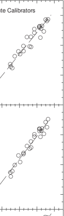
Figure 5: $B,R,I$ absolute magnitude–linewidth relations for 24 galaxies with independently determined distances from application of the Cepheid period–luminosity relation. The straight lines are the least squares best fits of the lines shown in Figs. 2 and 3.

The absolute calibration data are taken from Paper I ($B,R,I$) and from RSTW ($K^{\prime}$). In order to be consistent with the cluster template sample described in section 4 we restrict the calibration sample in luminosities to $M_{I}<-17.9$ and in inclinations to $i>45^{\circ}$ (2 galaxies initially thought to have $i>45^{\circ}$ but ultimately assigned inclinations slightly below $45^{\circ}$ are retained). Currently there are 24 galaxies which meet these criteria that have distances based on observations of Cepheid variable stars. Most of the observations were made with the Hubble Space Telescope (Freedman et al. 1997, Sandage et al. 1996, Tanvir et al. 1995, Newman et al. 1999). In order to be consistent, whenever possible the most recent distance provided by the HST Key Project Team is taken; ie. that given by Sakai et al. (1999). This reference includes distances from the team reanalysis of studies first-authored by Saha, Sandage, and Tanvir, respectively (Gibson et al. 1999). Sakai et al. also report on minor adjustments to the moduli of NGC’s 1365, 4535, and 4725 (Ferrarese et al. 1999). The $B,R,I$ luminosity–linewidth correlations are shown in Figure 5 for these 24 galaxies, where now absolute magnitudes are plotted based on the measured distances.

It is inappropriate to construct the luminosity–linewidth relation from the absolute calibration data alone because these galaxies do not constitute a complete sample. However if the calibrators are drawn from a similar distribution as the template objects, with no restriction in linewidths, then each of the 24 galaxies with independent distances provides a separate zero-point calibration of the template relations. The least-squares average provides the optimum fit and these are shown as the dashed lines in Fig. 5. Note the remarkable consistency. The slopes shown in Fig. 5 do not come from the absolute calibration data; rather they are given by the cluster templates. With only the one degree of freedom of the zero point, the scatter at $R$ and $I$ is only $\sim 0.24^{m}$. In Paper I, fits were made to the calibration sample alone with essentially identical slope and intercept determinations. This result strongly reinforces the hypothesis that the calibrators have similar properties to the cluster template galaxies.

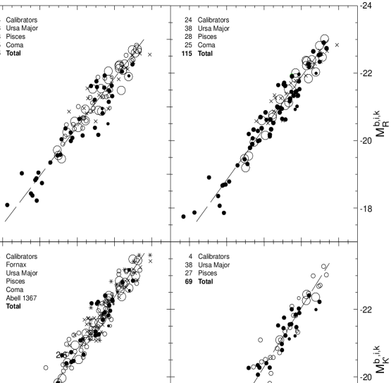
Figure 6: $B,R,I$, and $K^{\prime}$ absolute magnitude–linewidth relations for the cluster template galaxies translated to overlay on the zero-point calibrator galaxies. Symbols and straight line fits as in previous plots. The $I$ relation involves 5 clusters and 24 zero-point calibrators, the $B$ and $R$ relations are built with 3 clusters and 24 zero-point calibrators, and the $K^{\prime}$ relation is based on 2 clusters and 4 zero-point calibrators. Relative distances between clusters and with respect to the calibrators are the same on all plots.

The zero-points of the absolute relationships specify the distance moduli of the five template clusters. This information is used to superimpose the template relations on the absolute calibrators, as shown in Figure 6. Panel $c$ shows the $I$ band luminosity–linewidth relation with the 24 calibrators and the 155 cluster template galaxies shifted to the absolute magnitude scale of the calibrators. The $B$ and $R$ relations are shown in panels $a$ and $b$. In these cases 91 galaxies are available for the templates and there are the same 24 calibrators. Information at $K^{\prime}$ is more limited but consistent. RSTW provide $K^{\prime}$ photometry for four galaxies with Cepheid distances. The $K^{\prime}$ zero-point calibration can be seen in Figure 6$d$ with UMa and Pisces cluster data superimposed.

The agreement between bands is excellent. A measure of the agreement is given by the distance modulus in each band determined for the UMa cluster. The $I$ band analysis (155 template, 24 calibrators) gives shorter distances than the weighted mean by 0.02, the modulus at $B$ gives longer distances by 0.04, the modulus at $R$ is larger by 0.03 (for both bands: 91 template, 24 calibrators), and the modulus at $K^{\prime}$ is smaller by 0.05 (65 template, 4 calibrators). To obtain completely consistent results between bands, we average over the four bands with weights dependent on the square roots of the numbers of template and calibrator galaxies and the squares of dispersions. Relative weights are $B$:$R$:$I$:$K^{\prime}$= 0.46:0.66:1.00:0.25. Once these few percent corrections are made, the following calibrations are indicated:

$$M_{B}^{b,i,k}=-20.11-7.27({\rm log}W_{R}^{i}-2.5)$$ (5)

$$M_{R}^{b,i,k}=-21.12-7.65({\rm log}W_{R}^{i}-2.5)$$ (6)

$$M_{I}^{b,i,k}=-21.57-8.11({\rm log}W_{R}^{i}-2.5)$$ (7)

$$M_{K^{\prime}}^{b,i,k}=-23.17-8.78({\rm log}W_{R}^{i}-2.5)$$ (8)

The rms scatter: at $B$ $\pm 0.38$ template, $\pm 0.30$ calibrators; at $R$ $\pm 0.34$ template, $\pm 0.25$ calibrators; at $I$ $\pm 0.34$ template, $\pm 0.23$ calibrators; at $K^{\prime}$ $\pm 0.44$ template, $\pm 0.24$ calibrators. These results are consistent with those found in Papers I and II. The larger template scatter at $K^{\prime}$ appears to be partially due to the increased fractional representation of low luminosity systems.

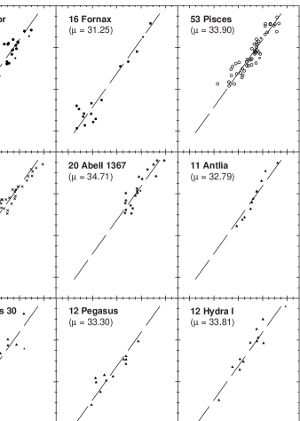
Figure 7: The $I$-band absolute magnitude–linewidth fits are shown separately for each of the clusters used in this study. The first 5 (panels $a$-$e$) contribute to the template relation. The remaining 7 (panels $f$-$l$: individual galaxies located by triangles) are given distances that follow from least squares fits to the template.

Figure 7$a-e$ presents $I$-band material for the five clusters that contribute to the template. Data for each cluster are plotted separately to show clearly the fits to the individual clusters. There is no evidence contrary to the hypothesis of a consistent luminosity–linewidth correlation from cluster to cluster, whatever the range of local environments.

7 The Hubble Constant

Now that the template relations have been converted to absolute scales, they can be used to determine distances to any appropriate galaxy or cluster sample. It would be dangerous to extrapolate for targets intrinsically less luminous than $M_{B}^{b,i,k}=-16.6^{m}$, $M_{R}^{b,i,k}=-17.6^{m}$, or $M_{I}^{b,i,k}=-17.9^{m}$, the low-luminosity limits of the template relations. If the goal is to measure H₀, these limits are of little concern because the clusters are chosen to be distant in order to minimize the effects of non-Hubble motions. Existing surveys of these clusters are limited to the more luminous members.

In a future paper we will apply the calibration described here and in Paper I to measure distances to hundreds of field galaxies in order to characterize the local velocity field. For the moment, with the interest of maintaining as homogeneous a set of measurements as possible, the H₀ determination will be based on the 5 clusters that went into the template plus 7 other clusters each with of order a dozen observed members. The photometric data come from Han (1992), Mathewson et al. (1992), and Giovanelli et al. (1997$a$). The fits are shown to the 7 additional clusters in Figure 7$f-l$. In these cases the samples are not complete. It has been argued above that each distance measurement is unbiased if the fit is done with the “inverse” regression, so the group distance moduli are given by the least squares minimization of the template regression on whatever information is available in the group. The distance moduli measured to individual galaxies in the 12 separate clusters are shown in Figure 8. As anticipated in the discussion of biases, the present analysis provides distances that are not dependent on magnitude. The effects seen by Bottinelli et al. (1986), Kraan-Korteweg et al. (1988), and Sandage (1994$a$) are not found. If there are tendencies for distance moduli to increase toward fainter magnitudes in the Antlia and Cancer samples, there are the opposite tendencies in the Coma and Pegasus samples. One could question if the former pair are better described by a steeper relation and the latter pair by a flatter relation. Bernstein et al. (1994) have suggested the Coma relation is flatter and shows less dispersion. However it is evident from the series of fits shown in Fig. 7 that the data can equally well be described by the single slope of the ensemble of the template galaxies. Deviations are within the expectations of statistical effects.

Results are summarized in Table 2 and Figure 9. The table provides (col. 2) the number of measures in the cluster, (col. 3) the rms scatter about the template relation, (col. 4/5) the distance modulus/distance of the cluster, (col. 6) the velocity of the cluster in the CMB frame as given by Giovanelli et al. (1997$a$), and (col. 7) the measure of H₀ from the cluster. The velocity given to the Pisces filament is the average of the values for the three main sub-condensations.

The error bars in Fig. 9 contain both distance and velocity components. The errors associated with distance depend directly on the rms dispersion in a cluster and inversely with the square root of the number of galaxies in the cluster sample. The error associated with velocity streaming is taken to be 300 km s^-1. The velocity component to the error is dominant inside 2000 km s^-1. The statistical errors in distance become the dominant factor beyond $\sim 6000$ km s^-1. The symbols in Fig. 9 specify different regions of the sky (see caption). There is a hint of systematic deviations: for example the filled circles (except for nearby Ursa Major) lie above the open circles. More data are clearly needed to address this possibility. For now, the best estimate of H₀ is derived by taking an average of log H₀ values with weights proportional to the inverse square of the error bars that are plotted. The result is H${}_{0}=77$ km s^-1 Mpc^-1.

7.1 Evaluation of Errors

What are the uncertainties? The present zero-point is based on the distance scale established by the Cepheid period-luminosity relation and the zero-point of that relation is based on a distance modulus of the Large Magellanic Cloud of 18.50. The 95% confidence accuracy of this scale is $\sim 10\%$ (Madore & Freedman 1998). There is also debate about a possible metallicity effect in the Cepheid luminosities (Kennicutt et al. 1998). Almost all the calibrators used here are more metal rich than the LMC. This possibility would lead to a correction of $\sim 5\%$ in the sense that H₀ would be reduced. An additional source of systematic error may arise from charge transfer effects within WFPC2 on HST (Stetson, private communication). Subsequent potential errors in color are amplified in the extinction-corrected Cepheid distance. Corrections could act to decrease the distances to those calibrators observed with HST and thereby increase the derived value of H₀ by $\sim 5\%$. There are problems in the reliance on the LMC because, not only is there uncertainty in its distance, but it is not the same kind of galaxy that otherwise interests us and the Cepheids are observed in the LMC with different instrumentation. Arguably a better alternative is to use NGC 4258 as the fundamental calibrator. A distant accurate to 7% is inferred from the geometry and motion of circum-nuclear masers (Herrnstein et al. 1999). This distance measurement bypasses the many steps of the distance ladder approach and the claimed accuracy is comparable to that touted for the LMC. NGC 4258 is a normal galaxy in our sample and the Cepheid population has been studied with HST (Maoz et al. 1999). The maser distance modulus of 29.29 differs from the Cepheid modulus based on the LMC calibration of 29.54 by $-$0.25 mag. If the scale established by the maser observations is used in preference to the LMC calibration then all moduli are reduced by $0.25^{m}$ and H₀ is increased by 12% from 77 to 86 km s^-1 Mpc^-1. It could be argued that the NGC 4258 calibration should be used in preference to the LMC calibration, or that one should average to get an intermediate result. We continue to use the LMC calibration simply to make comparisons easier with other work. All the uncertainties mentioned in this paragraph are intrinsic to the zero point and common to all but a few methods of determining extragalactic distances. These uncertainties at the level of $10-15\%$ are not included in the errors we quote that are related only to the current analysis.

Our biggest source of statistical uncertainty remains the zero-point calibration. The present discussion concerns the $B,R,I$ data. The considerably more uncertain $K^{\prime}$ calibration is discussed by RSTW. The fits illustrated in Fig. 5 are evaluated by tests involving the following reduced $\chi^{2}$ parameter:

$$\chi^{2}={\sum_{i}^{N}((M_{i}-M_{0,i})/\sigma_{cal})^{2}\over(N-1)}$$ (9)

where $M_{i}$ is the absolute magnitude of the $i^{th}$ of $N=24$ calibrators and $M_{0,i}=a+b({\rm log}W_{R,i}^{i}-2.5)$ is the expectation magnitude. The slope, $b$, is fixed to the template values of $-7.27$ at $B$, $-7.65$ at $R$, and $-8.11$ at $I$ and the zero-point, $a$ is varied. The dispersion, $\sigma_{cal}=0.24$, is taken from the fits shown in Fig. 5. The variation of $\chi^{2}$ with change of the zero-point is shown in Figure 10$a$. Then the linkage between the dependence on zero-point (the value of the correlation at ${\rm log}W_{R}^{i}=2.5$) and the inferred value of the Hubble Constant is shown in Figure 10$b$. The value at the minimum is normalized by the fit shown in Fig. 9. In $I$ band, the best case, the 95% probability level corresponds to an uncertainty of $\pm 6$ km s^-1 Mpc^-1 in the Hubble parameter ($\pm 8\%$). The $\chi^{2}$ tests at $B,R$ and $K^{\prime}$ are also shown.

The statistical uncertainties associated with the fits to the 12 clusters seen in Fig. 9 are somewhat smaller. The following $\chi^{2}$ evaluator was considered:

$$\chi^{2}={\sum_{i}^{N}w_{i}(({\rm logH}_{i}-{\rm logH}_{0})/\sigma_{clust})^{2}\over\sum_{i}^{N}w_{i}}$$ (10)

where ${\rm logH}_{i}$ is the measure of H₀ from the $i^{th}$ cluster, the weight is $w_{i}$, and $\sigma_{clust}=0.03$ is a typical value for the error bars in Fig. 9. The variation of $\chi^{2}$ with ${\rm logH}_{0}$ is shown in Figure 11. The 95% probability constraints are $\pm 5$ km s^-1 Mpc^-1 in the Hubble parameter ($\pm 6\%$).

The information available from the $B,R$ and $K^{\prime}$ relations is currently limited to only 2 clusters outside the Local Supercluster (1 at $K^{\prime}$) but is consistent with the $I$ distance measures at the level of 2%. The $K^{\prime}$ analysis by RSTW lead to a value of H${}_{0}=81$ km s^-1Mpc^-1. The 5% larger value comes almost entirely from use of only 1 cluster beyond the Local Supercluster rather than 10 in the case of the I-band. If the analysis at optical bands is restricted to exactly the same sample as that used at $K^{\prime}$ then H${}_{0}=80$ is found, essentially the same as the $K^{\prime}$ result.

Color plots provide a check of possible random or systematic errors in the data (see also Papers I and II). Figure 12 compares $I$ band results with those at $B,R$, and $K^{\prime}$. The $B-I$ panel contains a hint of a systematic effect, at the level of $0.1^{m}$, with Ursa Major galaxies redder than the mean and Pisces galaxies bluer than the mean. The Coma and calibrator galaxies are consistent with the mean. The Ursa Major and Pisces deviations have significances of $\sim 3\sigma$. The same effect is seen at $R-I$, with similar significances, though now the offsets are only at the level of $0.05^{m}$. The offsets remain marginally significant because the overall color–magnitude correlation is so tight at $R-I$. At $I-$$K^{\prime}$ the offsets between subsamples disappear. These small systematics could be explained if Galactic reddening is underestimated in the Ursa Major region and overestimated in the Pisces region by $E(B-V)\sim 0.04$ which is larger by a factor of 2 than the expected uncertainty. Another possibility is that there are systematic variations in the star formation histories of the various samples, but for the measurement of H₀ the problem is minor.

The measurement of inclinations (see section 2.2) remains one of the more problematic issues. However, the magnitude residuals from the $I$ band correlation shows no hint of dependency on inclination (see Figure 13). Substantially different extinction corrections produce results which agree at the level of 0.5% (section 2.4). It is particularly comforting that the $K^{\prime}$ results are consistent with the other bands since extinction issues are unimportant at that wavelength.

Galaxies of type Sa tend to lie below the mean relations (cf, Rubin et al. 1985, Pierce & Tully 1988; Verheijen 1997 discusses the issue in terms of the forms of rotation curves) and the small effect is seen in the plot of residuals versus type in Figure 14. See the small symbols in Fig. 7. The derived distances for the Sa systems are larger than the mean (see Fig. 8). This class is sufficiently few in number that the problem is ignored in the present analysis. The luminosity–linewidth relations are found to be consistent in environments as diverse as the Coma Cluster and the Pisces filament or the spiral-rich Ursa Major Cluster. Although environmental dependencies are possible, there is no evidence of any such effect.

Excluding uncertainty in the Cepheid scale, statistical errors added in quadrature amount to $\pm 8$ units of H₀ (95% confidence). The largest statistical error is still in the fit to the zero-point calibration. In Paper II we show that the residuals in the different bandpasses are highly correlated. Since the measurement errors in linewidth are small, it is implied that the scatter in the luminosity–linewidth correlation is either intrinsic or dominated by inclination corrections, particularly to the linewidths. Bothun & Mould (1987) and more recently Giovanelli et al. (1997$b$) provide a detailed description of the components of scatter in the luminosity–linewidth relation. Arguably the most intractable problem in terms of further improvements is in inclination measurements/corrections.

The current determination of H₀ is lower than in earlier days with the same methodology (eg, H${}_{0}=85$, Pierce & Tully 1988) and the primary reason is seen in Figure 15. There were only 5 calibrators available before the launch of Hubble Space Telescope and those 5 are seen to deviate by 0.31 mag in the mean (a 16% effect on distances). NGC 3031 has subsequently been reobserved with HST (Freedman et al. 1994) though the difference with the ground based result (Madore et al. 1993) is tiny. The remaining uncertainty in the charge transfer efficiency of the HST/WFPC2 CCDs could conceivably account for some of this offset, say up to 6%, but we have no reason to think that most of the effect is anything more than a statistical fluke.

8 Comparison with Literature Results

The turbulent history of Hubble Constant measurements has received its share of attention. If we restrict this discussion to just luminosity–linewidth determinations of H₀ and just those that have benefited from HST Cepheid calibrations, there is still the following remarkable range of results (all errors quoted from the original sources and usually $1\sigma$): Theureau et al. (1997) give H${}_{0}=53\pm 5$; Ekholm et al. (1999) give H${}_{0}=53_{-5}^{+6}$; Federspiel, Tammann, & Sandage (1998) give H${}_{0}=57\pm 7$; Watanabe, Ichikawa, & Okamura (1998) give H${}_{0}=65\pm 2_{-14}^{+20}$; Shanks (1997) gives H${}_{0}=69\pm 8$; Giovanelli et al. (1997$c$) give H${}_{0}=69\pm 5$; Sakai et al. (1999) give H${}_{0}=71\pm 4\pm 7$; and this paper gives H${}_{0}=77\pm 8$ (95%).

The straight average of these values is H${}_{0}=64\pm 9$. Why should we have much confidence in our lonely value on the high side? Several of the above-mentioned papers carried out quite sophisticated analyses. However there is no adequate substitute for good data. We will try to argue that our data are generally superior.

Consider the lowest estimates first. Both Theureau et al. (1997) and Ekholm et al. (1999) find H${}_{0}=53$. These collaborators draw data from the Lyon-Meudon Extragalactic Database, the source and extension of the Third Reference Catalogue (de Vaucouleurs et al. 1991). Magnitudes are at $B$ from many photographic or aperture photoelectric references, inclinations are mostly from the photographic sky surveys, and linewidths are from many sources and mixed quality. Several thousand galaxies are considered. Template relations are derived from field populations, broadened and distorted by velocity streaming. Theureau et al. work with the so-called ‘direct’ luminosity–linewidth relation, the correlation with errors in luminosity, and must deal with the full brunt of the Malmquist magnitude limit bias. Since the scatter is large with their mixed-bag data set, there is the potential for a large bias. One possible signature of a strong bias is an upturn in the measured H₀ at larger distances. However an upturn in H₀ could alternatively arise as a result of local structure; certainly plausible since we live in a filament and the gravity of the filament could be slowing the local expansion (e.g. Tully 1988). Theureau et al. (1997) follow the procedures of Bottinelli et al. (1986) who interpreted the upturn in H₀ as due to bias, not gravity, with the consequence that Bottinelli et al. inferred a low H₀. The Theureau et al. analysis is not as transparent but appears to rely on the same underlying assumption that there is a local regime where expansion actually represents the universal value and that the data sampling larger scales are biased. The fundamental problem is that their analysis procedure (use of the direct relation) requires bias corrections but the amplitude of the corrections can easily be disputed.

Ekholm et al. (1999) work with the ‘inverse’ luminosity–linewidth relation, as we advocate. They found H${}_{0}=72$ for the $B$ band relation (and H${}_{0}=78$ if diameters are substituted for luminosity). How could that result be reconciled with H${}_{0}=53$ from the direct relation? Ekholm et al. argue that reconciliation is possible if they assume that the Cepheid calibrators follow a relation with a different slope from that of galaxies in the field. Their justification for the slope difference is largely based on the aberrant location of one calibrator galaxy which is fainter than almost all $\sim 2000$ galaxies in their field sample (unidentified but probably NGC 3109). They argue that the different slope introduces a bias of 25% which they can correct for and assure us that their overall $1\sigma$ error budget is 10%. We would argue that if the calibrator and field slopes are different then the relations are different and just about anything is possible. Fortunately, with our own photometry there is no evidence that calibrators with known distances and other targets are drawn from different relations.

Federspiel et al. (1998) derive H${}_{0}=57$ from a distance they measure to the Virgo Cluster and a comparison with more distant clusters out as far as 11,000 km s^-1. The comparison with distant clusters uses information from Jerjen & Tammann (1993) that involves other input than the luminosity–linewidth method so we restrict ourselves here to the issue of the Virgo Cluster distance. Federspiel et al. also draw data from the same source as Theureau et al. and Ekholm et al. so it is data with a fair amount of scatter. Depth effects are a particular problem with the Virgo Cluster (Pierce & Tully 1988; Yasuda et al. 1997). The spiral population is probably experiencing substantial infall (Tully & Shaya 1984). There is evidence of considerable contamination from infalling groups on the far side of Virgo, projected onto the cluster and therefore indistinguishable in velocity. There are presently 7 galaxies in the Virgo Cluster region with Cepheid distance measurements. The individual moduli are 30.87, 30.95, 31.03, 31.04, 31.04, 31.10, and 31.80. The distance obtained for NGC 4639 is strongly deviant. The average of the first 6 (excluding NGC 4639) is $31.01\pm 0.08$. The deviation of NGC 4639 is 0.79 mag which puts it 7 Mpc in the background. It is at least plausible, if not probable, that NGC 4639 is in the background at the approximate distance of the so-called Virgo W^′ structure. If the true Virgo Cluster is at 16 Mpc as determined by the 6 galaxies with Cepheid distances excluding NGC 4639 then, all other other steps preserved, Federspiel et al. would have found H${}_{0}=74$. The merits of this background issue can be debated, but the Federspiel et al. value of H₀ rests on this tenuous point. Sandage (1994$b$) has found H${}_{0}=48\pm 5$ with the luminosity–linewidth method applied to field samples. That study predates the availability of HST Cepheid distances so will not be discussed further than to recall the discussion in section 3 and to say our additional criticisms would resemble those brought up in the Theureau et al. discussion.

Watanabe et al. (1998) find H${}_{0}=65$. With the revised calibrator distances of Sakai et al. (1999) they would have gotten 67. The photometry for their field samples comes from photographic material at $B$-band but at least the source is homogeneous and is calibrated with CCD imaging. The source for HI linewidths is also homogeneous. The maximum likelihood analysis has merit. Watanabe et al. had 10 calibrators with Cepheid distances available. If they used all 10 and converted to the Sakai et al. distance revisions then they would have obtained H${}_{0}=69$. They prefer not to use 5 of these calibrators because of issues having to do with the detailed velocity fields or inclination ambiguities. They reject half their calibrators on criteria that are not applied to their field sample. We use the calibrators they reject, so we feel the appropriate Watanabe et al. result to compare with our own is H${}_{0}=69$. Even so, the Watanabe et al. result is 10% lower than our value, barely within our 95% uncertainty. One possibility for the remaining discrepancy might lie in the use of heterogeneous data for the calibration sample. Are the magnitude, inclination, and linewidth parameters that they take from the literature really all on the same system as their field sample?

As an aside, note that we almost never reject candidates that satisfy magnitude and inclination constraints and are typed later than Sa. In a small number of cases extremely pathological or interacting galaxies are rejected a priori. In the current template plus calibrator sample, only 2 of 181 initial candidates were rejected because of $>4\sigma$ deviance. All available galaxies with Cepheid distances are used.

Shanks (1997) finds H${}_{0}=69$. To facilitate a comparison with the present work, consider only the luminosity–linewidth analysis by Shanks (ie, not the analysis based on SN I$a$ distances), reject NGC 4496A not used in the current paper because of its face-on inclination, and update the Cepheid distances used to those in the current paper (including those by Gibson et al. 1999). With these changes, Shanks would have found H${}_{0}=73$, within $1\sigma$ of our present result.

Giovanelli et al. (1997$c$) also get H${}_{0}=69$. Six of their 12 calibrators have revised distances in Sakai et al. (1999), whence H${}_{0}=70$. This result is only marginally consistent with what we find in spite of a big overlap in data. We made a concerted effort to track down the systematic difference with only partial success. There is good consistency between our raw magnitudes, inclinations and linewidths. A problem arises with extinction corrections to magnitudes (discussed in section 2.4) but the analyses were carried out with our alternate prescriptions and each produces the same results if carried out consistently across templates and calibrators. A nuance of the bias problem does generate a 5% effect that, if our viewpoint is accepted, takes Giovanelli et al. to H${}_{0}=73$. Those authors use a maximum likelihood fitting procedure that requires bias corrections, unlike our procedure. However, upon fitting to the zero-point calibrators with their procedure it is necessary to again account for biases because lower luminosity galaxies are badly under represented among the calibrators. However, in this case the sense of the correction now has the opposite sign, increasing the Hubble Constant. Evidently Giovanelli et al. did not make this correction. A $\Delta{\rm H}_{0}=4$ km s^-1 Mpc^-1 difference remains between us. This difference would not seem bad except our data sets have so much overlap that the origins of this 5% offset should be evident. A mystery remains.

Finally, the HST Key Project Team (Sakai et al. 1999) report H${}_{0}=71$. They use three major data sets. Their acknowledged best data set is at $I$ band and has a large overlap with the material used by Giovanelli et al. (1997$c$) and ourselves. From this material alone, Sakai et al. find H${}_{0}=74$. A second smaller data set at $B$ and $V$ bands gives Sakai et al. H${}_{0}=70$. The historic Aaronson et al. (1982, 1986) data sets using aperture $H_{-0.5}$ band photometry gives H${}_{0}=67$. At $I$ band where the data are best and the data overlap is substantial, there is good agreement between Sakai et al. and ourselves. The agreement is marginal with their $B,V$ results and poor with their $H_{-0.5}$ results. The situation is perplexing. Sakai et al. find an indication of a problem with $I-H_{-0.5}$ color differences in the unphysical sense that their calibrators are redder than their cluster galaxies. At least in our analysis there is consistency between results at $B,R,I$, and $K^{\prime}$.

The results presented in this paper are at least marginally consistent with the other studies that use high quality data. Once we are on the same page with assumed distances to calibrators, the Watanabe et al., Shanks, Giovanelli et al., and Sakai et al. results are lower by $1-2\sigma$. There are several features of the present study that arguably make it better than others. For one thing, the photometric material on the local calibrators that is introduced in Paper I was obtained with fields sufficiently larger than the target galaxies that they give good sky definition. Second, we observed near, big galaxies and distant, small galaxies with common filters and procedures and have substantial sample overlaps with other programs so there should be a reliable bridge between near and distant. Third and foremost, only in this study is there serious consideration given to the issue of magnitude completion in the template construction. Only if this issue is properly addressed can one then use the ‘inverse’ luminosity–linewidth relations with nulled biases. Both Giovanelli et al. and Sakai et al. have constraints on linewidths that make corrections for biases difficult. It is this simplification of the bias analysis through attention to the template calibration that, we claim, gives us an advantage over the other teams with comparably good data.

It is most remarkable that the slopes derived from the template relations when slid to fit the Cepheid calibrators, with only freedom in the zero point, result in $R$ and $I$ scatter of only $0.24^{m}$.

Endless comparisons could be made with other techniques used to derive H₀. If one asks which is the single result that causes us the most concern, it would be the determination of H₀ with supernova of type I$a$. For example, Riess, Press, & Kirshner (1996) find H${}_{0}=64\pm 6$ ($2\sigma$ uncertainty). However the Cepheid distances to the SN I$a$ host galaxies that were available to Riess et al. (NGC 4536: Saha et al. 1996; NGC 4639: Sandage et al. 1996; NGC 5253: Sandage et al. 1994) have now been re-evaluated by the HST Key Project Team (Gibson et al. 1999). If only we use the new Cepheid distances given by the Key Project Team in preference to the distances given by Saha and Sandage then the Riess et al. value for H₀ is increased from 64 to 73. The Key Project Team do a more complete calibration of the SN I$a$ procedure with 7 calibrating galaxies and find H${}_{0}=68\pm 4$ ($2\sigma$ statistical uncertainty). At least our error bars overlap with the SN I$a$ results.

No single-point failure of the luminosity–linewidth analysis is likely to produce a systematic error greater than 5%. Conspiratorial addition of several independent systematic errors is possible. Uncertainties in the Cepheid calibration (LMC distance, metallicity effects, reddening, crowded field photometry, LMC calibration relation) are another matter and we take what we are given. Replacing the LMC calibration with the NGC 4258 calibration gives a 12% larger value of H${}_{0}=86$. It is possible that the value of the Hubble parameter determined nearby may not reflect the cosmological value, a manifestation of the local velocity anomaly problem on a larger scale. For example, Zehavi et al. (1999) raise the possibility that we live in an underdense region that extends out to $\sim 6000$ km s^-1, whence H₀ would be perhaps 6% lower than the locally measured value. Such a possibility can be entertained though there is no evidence for a dependence of H₀ with distance out to $\sim 19,000$ km s^-1 from the luminosity–linewidth analysis of Giovanelli et al. (1999). To conclude, this study determines a value of the Hubble Constant of H${}_{0}=77\pm 8$ km s^-1 Mpc^-1. The error is the 95% probable statistical error. Cummulative systematic errors within the present analysis could amount to as much as 10%. The zero point external to this analysis is still uncertain by $\sim 10\%$.

The only substantial change in the last decade in the measure of H₀ from the luminosity–linewidth method has resulted from the five times larger number of zero-point calibrators. Curiously, the galaxies with Cepheids observed from the ground lie $0.3^{m}$ fainter than the ensemble mean dominated by the galaxies observed with HST. Perhaps this difference is only a statistical fluke.

9 Acknowledgments

Jo Ann Eder processed Arecibo HI observations that were made at our request of several galaxies in the Coma Cluster. Other unpublished HI line profiles were made available to us by Martha Haynes, Barbara Williams, and Wolfram Freudling.

Table 1: Data for 24 Calibrators and 155 Galaxies in 12 Clusters

Table 2: Five Template Clusters and Seven More

Cluster	No.	RMS	Modulus	Distance	$V_{cmb}$	H0
		(mag)	(mag)	(Mpc)	(km/s)	(km/s/Mpc)
Fornax	16	0.50	31.25	17.8	1321	74
Ursa Major	38	0.40	31.35	18.6	1101	59
Pisces Filament	53	0.35	33.90	60.3	(4779)	79
Coma	28	0.34	34.68	86.3	7185	83
Abell 1367	20	0.36	34.71	87.5	6735	77
Antlia	11	0.27	32.79	36.1	3120	86
Centaurus 30	13	0.60	33.02	40.2	3322	83
Pegasus	12	0.40	33.30	45.7	3519	77
Hydra I	12	0.36	33.81	57.8	4075	70
Cancer	15	0.38	33.96	61.9	4939	80
Abell 400	7	0.19	34.81	91.6	6934	76
Abell 2634	16	0.36	35.23	111.2	7776	70
Weighted average						77

Figure 1: $I$-band apparent magnitude–HI profile linewidth plots for the five clusters that contribute to the template luminosity–linewidth correlations. Magnitudes are adjusted for internal and Galactic absorption and small redshift corrections. Large symbols: types Sab and later. Small symbols: type Sa. The Ursa Major and Fornax samples are complete to $I_{T}^{b,i,k}=13.4$. The Coma, Abell 1367, and Pisces filament samples are nearly complete to $I_{T}^{b,i,k}=13.8$. Galaxies fainter than these limits are excluded.

Figure 2: $I$-band apparent magnitude–linewidth relations for 5 clusters translated to the Ursa Major relation. Symbols as in Fig. 1. The straight line is a least squares fit to the ensemble with errors in linewidths after the iterations described in the text.

Figure 3: $B$ and $R$ apparent magnitude–linewidth relations for 3 clusters translated to the Ursa Major relation with the same relative distances assumed with the $I$-band material. Symbols as in Figs. 1 and 2. The straight lines are least squares fits to the ensemble with errors in linewidths.

Figure 4: $K^{\prime}$  apparent magnitude–linewidth relations for 2 clusters, with Pisces translated to the Ursa Major relation with the same relative distances assumed with the $I$-band material. Symbols as in Figs. 1 and 2. The straight line is a least squares fits to the ensemble with errors in linewidths.

Figure 8: Distance moduli of individual cluster galaxies versus $I$ magnitude. Symbols as in previous figures.

Figure 9: Values for the Hubble parameter determined for each of the 12 clusters plotted against the cluster velocity in the microwave background frame. Errors are a convolution of the statistical errors in distance and an uncertainty of 300 km s^-1 in velocities. Symbols depend on location in the sky: filled circles: north celestial and north galactic, open circles: north celestial and south galactic, filled squares: south celestial and north galactic, open squares: south celestial and south galactic.

Figure 10: Reduced $\chi^{2}$ goodness-of-fits tests. In panel $a$, $\chi^{2}$ values are recorded as the cluster template relations are translated in zero-point. In panel $b$, the sensitivity of $\chi^{2}$ on the choice of H₀ is shown. The heavy solid curve is for the best case $I$ band data. The curve for the $K^{\prime}$ data is carried over from RSTW.

Figure 11: The $\chi^{2}$ dependency of the fit to 12 clusters illustrated in Fig. 8. Weights are a function of the error bars in that figure.

Figure 12: Color–magnitude diagrams. Left: $B-I$. Center: $R-I$. Right: $I-$$K^{\prime}$. Symbols as in previous plots. Long dashed lines are the regressions with errors in colors. Dotted lines are the double regressions.

Figure 13: Deviations from the $I$ band luminosity–linewidth correlation as a function of inclination. Symbols have the same meanings as in Figs. 6 and 7. The dashed lines indicate the $2\sigma$ deviation boundaries.

Figure 14: Deviations from the $I$ band luminosity–linewidth correlation as a function of morphological type. Symbols have the same meanings as in Figs. 6, 7, and 13. The dashed lines indicate the $2\sigma$ deviation boundaries.

Figure 15: Deviations from the $I$ band luminosity–linewidth correlation for the calibrator galaxies, distinguishing by source of the distance estimate. Source 1 (open circles): ground based Cepheid observations; source 2 (filled circles): HST Key Project Cepheid observations; source 3 (filled squares): HST Cepheid observations by first authors Sandage, Saha, or Tanvir reanalyzed by the Key Project Team; source 4: HST Cepheid observations in NGC 4603 (open triangle) and in NGC 4258 (filled triangle).

References

- (1)
- (2) Aaronson, M., Huchra, J.P., & Mould, J.R. 1979, ApJ, 229, 1
- (3)
- (4) Aaronson, M., Bothun, G., Mould, J.R., Huchra, J.P., Schommer, R.A., & Cornell, M.E. 1986, ApJ, 302, 536
- (5)
- (6) Aaronson, M., Huchra, J.P., Mould, J.R., Tully, R.B., Fisher, J.R., van Woerden, H., Goss, W.M., Chamaraux, P., Mebold, U., Siegman, B., Berriman, G., & Persson S.E. 1982, ApJS, 50, 241
- (7)
- (8) Begeman, K.G. 1989, A&A, 223, 47
- (9)
- (10) Bernstein, G.M., Guhathakurta, P., Raychaudhury, S., Giovanelli, R., Haynes, M.P., Herter, T., & Vogt, N.P. 1994, AJ, 107, 1962
- (11)
- (12) Bosma, A., & Freeman, K.C. 1993, AJ, 106, 1394
- (13)
- (14) Bottinelli, L., Gouguenheim, L., Paturel, G., & de Vaucouleurs, G. 1983, A&A, 118, 4
- (15)
- (16) Bottinelli, L., Gouguenheim, L., Paturel, G., & Teerikorpi, P. 1986, A&A, 156, 157
- (17)
- (18) Braine, J., Combes, F., & van Driel, W. 1993, A&A, 280, 451
- (19)
- (20) Broeils, A.H. 1992, Ph.D. thesis, University of Groningen
- (21)
- (22) Bureau, M., Mould, J.R., & Staveley-Smith, L. 1996, ApJ, 463, 60
- (23)
- (24) Cayatte, V., van Gorkom, J.H., Balkowski, C., & Kotanyi, C. 1990, AJ, 100, 604
- (25)
- (26) Courteau, S. 1997, AJ, 114, 240
- (27)
- (28) de Vaucouleurs, G., de Vaucouleurs, A., Corwin, H.G. Jr., Buta, R.J., Paturel, G., & Fouqué, P. 1991, Third Reference Catalogue of Bright Galaxies (New York: Springer)
- (29)
- (30) Ekholm, T., Teerikorpi, P., Theureau, G., Hanski, M., Paturel, G., Bottinelli, L., & Gouguenheim, L. 1999, A&A, 347, 99
- (31)
- (32) Federspiel, M., Tammann, G.A., & Sandage, A. 1998, ApJ, 495, 115
- (33)
- (34) Ferrarese, L., Mould, J.R., Kennicutt, R.C. Jr., Huchra, J., Ford, H.C., Freedman, W.L., Stetson, P., Madore, B.F., Sakai, S., Gibson, B.K, Graham, J.A., Hughes, S.M., Illingworth, G.D., Kelson, D.D., Macri, L.M., Sebo, K., & Silbermann, N.A. 1999, ApJ, astro-ph/9908192
- (35)
- (36) Fouqué, P., Bottinelli, L., Durand, N., Gouguenheim, L., & Paturel, G. 1990, A&A, 86, 473
- (37)
- (38) Freedman, W.L., Hughes, S.M., Madore, B.F., Mould, J.R., Lee, M.G., Stetson, P., Kennicutt, R.C. Jr., Turner, A., Ferrarese, L., Ford, H.C., Graham, J.A., Hill, R., Hoessel, J.G., Huchra, J., & Illingworth, G.D. 1994, ApJ, 427, 628
- (39)
- (40) Freedman, W.L., Mould, J.R., Kennicutt, R.C. Jr., & Madore, B.F. 1997, in IAU Symp. 183: Cosmological Parameters and the Evolution of the Universe, p. 17.
- (41)
- (42) Garcia-Barreto, J.A., Downes, D., & Huchtmeier, W.K. 1994, A&A, 288, 705
- (43)
- (44) Gavazzi, G. 1989, ApJ, 346, 59
- (45)
- (46) Gibson, B.K, Stetson, P.B., Freedman, W.L., Mould, J.R., Kennicutt, R.C. Jr., Huchra, J.P., Sakai, S., Graham, J.A., Fassett, C.I., Kelson, D.D., Ferrarese, L., Hughes, S.M., Illingworth, G.D., Macri, L.M., Madore, B.F., Sebo, K.M., & Silbermann, N.A. 1999, ApJ, astro-ph/9908192
- (47)
- (48) Giovanelli, R., Dale, D., Haynes, M., Hardy, E., & Campusano, L. 1999, ApJ, (Nov), astro-ph/9906362
- (49)
- (50) Giovanelli, R., Haynes, M.P., da Costa, L.N., Freudling, W. Salzer, J.J., & Wegner, G. 1997, ApJ, 477, L1
- (51)
- (52) Giovanelli, R., Haynes, M.P., Herter, T., Vogt, N.P., da Costa, L.N., Freudling, W., Salzer, J.J., & Wegner, G. 1997, AJ, 113, 53
- (53)
- (54) Giovanelli, R., Haynes, M.P., Herter, T., Vogt, N.P., Wegner, G., Salzer, J.J., da Costa, L.N., & Freudling, W. 1997, AJ, 113, 22
- (55)
- (56) Giovanelli, R., Haynes, M.P., Salzer, J.J., Wegner, G., da Costa, L.N., & Freudling, W. 1995, AJ, 110, 1059
- (57)
- (58) Han, M.S. 1992, ApJS, 81, 35
- (59)
- (60) Han, M.S. & Mould, J.R. 1992, ApJ, 396, 453
- (61)
- (62) Haynes, M.P., & Giovanelli, R. 1991, ApJS, 77, 337
- (63)
- (64) Haynes, M.P., & Giovanelli, R. 1991, AJ, 102, 841
- (65)
- (66) Haynes, M.P., Giovanelli, R., Herter, T., Vogt, N.P., Freudling, W., Maia, M.A.G., Salzer, J.J., & Wegner, G. 1997, AJ, 113, 1197
- (67)
- (68) Harris, W.E., Durrell, P.R., Pierce, M.J., & Secker, J. 1998, Nature, 395, 45
- (69)
- (70) Herrnstein, J.R., Moran, J.M., Greenhill, L.J., Diamond, P.J., Inoue, M., Nakai, N., Miyoshi, M., Henkel, C., & Riess, A. 1999, Nature, 400, 539
- (71)
- (72) Holmberg, E. 1958, Medd. Lunds Astron. Obs., Ser. II, No. 126
- (73)
- (74) Huchtmeier, W. & Richter, O-G. 1989, A General Catalogue of HI Observations of Galaxies (Springer-Verlag)
- (75)
- (76) Jacoby, G.H., Ciardullo, R., & Ford, H.C 1990, ApJ, 356, 332
- (77)
- (78) Jensen, J.B., Tonry, J.L., & Luppino, G.A. 1998, ApJ, 505, 111
- (79)
- (80) Jerjen, H., & Tammann, G.A. 1993, A&A, 276, 1
- (81)
- (82) Kennicutt, R.C. Jr, Freedman, W.L., & Mould, J.R. 1995, AJ, 110, 1476
- (83)
- (84) Kennicutt, R.C. Jr, Stetson, P.B., Saha, A., Kelson, D., Rawson, D.M., Sakai, S., Madore, B.F., Mould, J.R., Freedman, W.L., Bresolin, F., Ferrarese, L., Ford, H., Gibson, B.K., Graham, J.A., Han, M., Harding, P., Hoessel, J.G., Huchra, J.P., Hughes, S.M.G., Illingworth, G.D., Macri, L.M., Phelps, R.L., Silbermann, N.A., Turner, A.M., & Wood, P.R. 1998, ApJ, 498, 181
- (85)
- (86) Kraan-Korteweg, R.C., Cameron, L.M., & Tammann, G.A. 1988, ApJ, 331, 620
- (87)
- (88) Madore, B.F., & Freedman, W.L. 1995, AJ, 109, 1645
- (89)
- (90) Madore, B.F., & Freedman, W.L. 1998, ApJ, 492, 110
- (91)
- (92) Madore, B.F., Freedman, W.L., & Lee, M.G. 1993, AJ, 106, 2243
- (93)
- (94) Magri, C. 1990, Ph.D. thesis, Cornell University
- (95)
- (96) Malmquist, K.G. 1920, Medd. Lunds Ast. Obs. Series II, no. 22
- (97)
- (98) Maoz, E., Newman, J.A., Ferrarese. L., Stetson, P.B., Zepf, S.E., Davis, M., Freedman, W.L., & Madore, B.F. 1999, Nature, 401, 451
- (99)
- (100) Mathewson, D.S, Ford, V.L, & Buchhorn, M. 1992, ApJS, 81, 413
- (101)
- (102) Mould, J.R., Akeson, R.L., Bothun, G.D., Han, M., Huchra, J.P., Roth, J., & Schommer, R.A. 1993, ApJ, 409, 14
- (103)
- (104) Newman, J.A., Zepf, S.E., Davis, M., Freedman, W.L., Madore, B.F., Stetson, P.B., Silbermann, N., & Phelps, R. 1999, ApJ, 523, 506
- (105)
- (106) Pierce, M.J., & Tully, R.B. 1988, ApJ, 330, 579
- (107)
- (108) Pierce, M.J., & Tully, R.B. 1992, ApJ, 387, 47
- (109)
- (110) Pierce, M.J., & Tully, R.B. 1999, in preparation (Paper I)
- (111)
- (112) Pierce, M.J., & Tully, R.B. 1999, in preparation (Paper II)
- (113)
- (114) Puche, D., Carignan, C., & Bosma, A. 1990, AJ, 100, 1468
- (115)
- (116) Riess, A.G., Press, W.H., & Kirshner, R.P. 1996, ApJ, 473, 88
- (117)
- (118) Rood, H.J., & Williams, B.A. 1993, MNRAS, 263, 211
- (119)
- (120) Roth, J., Mould, J.R., & Davies, R.D. 1991, AJ, 102, 1303
- (121)
- (122) Rothberg, B., Saunders, W., Tully, R.B., & Witchalls, P.L. 1999, ApJ, 000, 000 (RSTW)
- (123)
- (124) Saha, A., Sandage, A., Labhardt, L., Tammann, G.A., Macchetto, F.D., & Panagia, N. 1996, ApJ, 466, 55
- (125)
- (126) Sakai, S., Giovanelli, R., & Wegner, G. 1994, ApJ, 108, 33
- (127)
- (128) Sakai, S., Mould, J.M, Hughes, S.M.G., Huchra, J.P., Macri, L.M., Kennicutt, R.C. Jr., Gibson, B.K., Ferrarese, L., Freedman, W.L., Han, M., Ford, H.C., Graham, J.A., Illingworth, G.D., Kelson, D.D., Madore, B.F., Saha, A., Sebo, K., Silbermann, N.A., & Stetson, P.B. ApJ, astro-ph/9909269
- (129)
- (130) Sandage, A. 1994, ApJ, 430, 1
- (131)
- (132) Sandage, A. 1994, ApJ, 430, 13
- (133)
- (134) Sandage, A. 1999, AJ, 117, 157
- (135)
- (136) Sandage, A., Saha, A., Tammann, G.A., Labhardt, L., Schwengler, H., Panagia, N., & Macchetto, F.D. 1994, ApJ, 423, L13
- (137)
- (138) Sandage, A., Saha, A., Tammann, G.A., Labhardt, L., Panagia, N., & Macchetto, F.D. 1996, ApJ, 460, L15
- (139)
- (140) Schechter, P.L. 1980, AJ, 85, 801
- (141)
- (142) Schlegel, D., Finkbeiner, D., & Davis, M. 1998, ApJ, 500, 525
- (143)
- (144) Schneider, S.E., Thuan, T.X., Magri, C., & Wadiak, J.E. 1990, ApJS, 72, 245
- (145)
- (146) Schneider, S.E., Thuan, T.X., Mangum, J.G., & Miller, J. 1992, ApJS, 81, 5
- (147)
- (148) Scodeggio, M., & Gavazzi, G. 1993, ApJ, 409, 110
- (149)
- (150) Shanks, T. 1997, MNRAS, 290, L77
- (151)
- (152) Shaya, E.J., Peebles, P.J.E., & Tully, R.B. 1995, ApJ, 454, 15
- (153)
- (154) Tanvir, N.R., Shanks, T., Ferguson, H.C., & Robinson, D.R.T. 1995, Nature, 377, 27
- (155)
- (156) Teerikorpi, P. 1984, A&A, 141, 407
- (157)
- (158) Theureau, G., Hanski, M., Ekholm, T., Bottinelli, L., Gouguenheim, L., Paturel, G., & Teerikorpi, P. 1997, A&A, 322, 730
- (159)
- (160) Tonry, J.L, Blakeslee, J.P., Ajhar, E.A., & Dressler, A. 1997, ApJ, 475, 399
- (161)
- (162) Tonry, J.L, Blakeslee, J.P., Ajhar, E.A., & Dressler, A. 1999, astro-ph/9907062
- (163)
- (164) Tully, R.B. 1988, Nature, 334, 209
- (165)
- (166) Tully, R.B. 1988, in The Extragalactic Distance Scale, Eds. S. van den Bergh and P.J. Pritchet, ASP Conf. Ser. 4, 318
- (167)
- (168) Tully, R.B., & Fisher, J.R. 1977, A&A, 54, 661
- (169)
- (170) Tully, R.B., & Fouqué, P. 1985, ApJS, 58, 67
- (171)
- (172) Tully, R.B., Mould, J.M., & Aaronson, M. ApJ, 257, 527
- (173)
- (174) Tully, R.B., Pierce, M.J., Huang, J.S., Saunders, W., Verheijen, M.A.W., & Witchalls, P.L. 1998, AJ, 115, 2264
- (175)
- (176) Tully, R.B., & Shaya, E.J. 1984, ApJ, 281, 31
- (177)
- (178) Tully, R.B., & Verheijen, M.A.W. 1997, ApJ, 484, 145
- (179)
- (180) Tully, R.B., Verheijen, M.A.W., Pierce, M.J., Huang, J.S., & Wainscoat, R.J. 1996, AJ, 112, 2471
- (181)
- (182) Verheijen, M.A.W. 1997, Ph.D. thesis, University of Groningen
- (183)
- (184) Watanabe, M., Ichikawa, T., & Okamura, S. 1998, ApJ, 503, 553
- (185)
- (186) Wegner, G., Haynes, M.P., & Giovanelli, R. 1993, AJ, 105, 1251
- (187)
- (188) Willick, J.A. 1994, ApJS, 92, 1
- (189)
- (190) Willick, J.A., Courteau, S., Faber, S.M., Burstein, D., Dekel, A., & Kolatt, T. 1996, ApJ, 457, 460
- (191)
- (192) Willick, J.A, Courteau, S., Faber, S.M., Burstein, D., Dekel, A., & Strauss, M.A. 1997, ApJS, 109, 333
- (193)
- (194) Willick, J.A., & Strauss, M.A. 1998, ApJ, 507, 64
- (195)
- (196) Yasuda, N., Fukugita, M., & Okamura, S. 1997, ApJS, 108, 417
- (197)
- (198) Zehavi, I., Riess, A.G., Kirshner, R.P., & Dekel, A. 1998, ApJ, 503, 483
- (199)