MHD Turbulence in Star-Forming Clouds

Abstract

We review how supersonic turbulence can both prevent and promote the collapse of molecular clouds into stars. First we show that decaying turbulence cannot significantly delay collapse under conditions typical of molecular clouds, regardless of magnetic field strength so long as the fields are not supporting the cloud magnetohydrostatically. Then we review possible drivers and examine simulations of driven supersonic and trans Alfvénic turbulence, finally including the effects of self-gravity. Our preliminary results show that, although turbulence can support regions against gravitational collapse, the strong compressions associated with the required velocities will tend to promote collapse of local condensations.

1 Introduction

A fundamental unanswered question in star formation is why stars do not form faster than they are currently thought to. The free-fall times $t_{\rm ff}$ of molecular clouds with typical densities are

$$t_{\rm ff}=(3\pi/32G\rho)^{1/2}=(1.2\times 10^{6}\mbox{ yr})(n/10^{3}\mbox{ cm}^{-3})^{-1/2},$$ (1)

where $n$ is the number density of the cloud, and I take the mean molecular mass $\mu=3.32\times 10^{-24}$ g.

In contrast to these Myr collapse times, molecular clouds are commonly thought to be tens of Myr old (e. g. Blitz & Shu 1980). This lifetime is derived from such considerations as their locations downstream from spiral arms, the ages of stars apparently associated with them, and their overall frequency in the galaxy.

Either molecular cloud lifetimes are much shorter than commonly supposed, or they are supported against gravitational collapse by some mechanism, presumably related to the supersonic random velocities observed in them. The first possibility has very recently received an intriguing examination by Ballesteros-Paredes, Hartmann, & Vázquez-Semadeni (1999); however the remainder of this paper will concern itself with the second possibility.

Support mechanisms that have been proposed over the years have included decaying turbulence from the formation of the clouds, magnetic fields and MHD waves, and continuously driven turbulence. Each of these raises questions: how can the decay of decaying turbulence be drawn out over such long periods; can magnetohydrostatically supported regions collapsing by ambipolar diffusion reproduce the observations of molecular cloud cores (Nakano 1998); and what could be the energy source for continuously driven turbulence?

The usual formulation of the problem with maintaining turbulence arising from initial conditions is that the turbulence is measured to be strongly supersonic, and shocks are well known to dissipate energy quickly. Arons & Max (1975) were among the first to suggest that magnetic fields might solve this problem if they were strong enough to reduce shocks to Alfvén waves, since ideal linear Alfvén waves lose energy only to resistive dissipation. As we will review in more detail below, Mac Low et al. (1998) showed that a more realistically computed mix of MHD waves is not nearly so cooperative, a result confirmed by Stone, Ostriker, & Gammie (1998).

On the other hand, if the observed motions come from driving, then the energy source needs to be identified, the amount of energy it is contributing must be determined, and how to couple the energy source to the motions of the dense gas must be explained. Any clues we can derive from comparison of turbulence simulations to observations are helpful (see Mac Low & Ossenkopf 1999 and Rosolowsky et al. 1999 for recent attempts to do that).

2 Computations

In the rest of this paper we will present computations of compressible turbulence with and without magnetic fields and self-gravity. For most of the models we use the astrophysical MHD code ZEUS-3D (Stone & Norman 1992a, b; Clarke 1994). This is a second-order code using Van Leer (1977) advection that evolves magnetic fields using a constrained transport technique (Evans & Hawley 1988) as modified by Hawley & Stone (1995), and that resolves shocks using a von Neumann artificial viscosity. We also use a smoothed particle hydrodynamics (SPH) code (e. g. Benz 1990; Monaghan 1992) with a different formulation of the von Neumann viscosity as a comparison to our hydrodynamical models.

All of our models are set up in cubes with periodic boundary conditions and initially uniform density and, in MHD cases, magnetic field. We use an isothermal equation of state for the gas, which is a good approximation for molecular gas between number densities of $10^{2}$ cm^-3 and $10^{9}$ cm^-3 typical of molecular clouds. A pattern of Gaussian velocity perturbations is then imposed on the gas, with the spectrum defined in wavenumber space as desired. Decaying models are then left to evolve (Mac Low et al. 1998), while driven models have the same fixed pattern added in every time step with a varying amplitude computed to ensure a constant rate of kinetic energy input over time (Mac Low 1999). Models with self-gravity use an FFT solver to integrate the Poisson equation.

3 Decaying Turbulence

We used models of decaying turbulence to address the question of whether magnetic fields could significantly decrease the dissipation rate of supersonic turbulence, as described in Mac Low et al. (1998). For these models, we set up an initial velocity perturbation spectrum that was flat in $k$-space and extended from $k=2$ to $k=8$. Although $k^{-2}$ spectra are often used to drive supersonic turbulence, a spectrum of Gaussian perturbations with this $k$-dependence is not a good match to a box full of shocks with a $k^{-2}$ spectrum—in the latter case the dependence is just the Fourier transform of a step function.

In Figure 1 we show examples of cuts through 3D models of decaying turbulence computed with ZEUS at resolutions of $128^{3}$ and $256^{3}$ (Mac Low 1999). Although these are cuts rather than column density images, the tendency for the shock waves to form filamentary structures reminiscent of molecular clouds can be clearly seen.

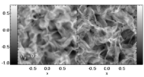
XS

Figure 1: Cuts through 3D supersonic turbulence models decaying from an initial rms velocity of Mach 5, after 0.2 sound crossing times. The model on the left was computed with $128^{3}$ zones, while the model on the right was computed with $256^{3}$ zones. The greyscale is labeled for log of density

We measured the total kinetic energy on the grid over time for these models, as shown in Figure 2(a). For comparison, we also performed a resolution study using SPH, shown in Figure 2(b). We found that the kinetic energy decays as $t^{-\eta}$, with $0.85<\eta<1.1$ for models in the supersonic regime (Mach numbers in the range from roughly 1 to 5). This decay rate is actually somewhat slower than the decay rate for incompressible, subsonic turbulence, which, according to the theory of Kolmogorov (1941), decays with $\eta\sim 5/3$.

Figure 2: Decay rate of kinetic energy over time for 3D computations with initial Mach number of 5. (a) hydrodyamical with ZEUS (b) hydrodynamical with SPH (c) MHD with Alfvén speed $v_{A}=c_{s}$ (d) MHD with $v_{A}=0.2c_{s}$. ZEUS models (a,c,d) were done with $32^{3}$ (dotted), $64^{3}$ (short-dashed), $128^{3}$ (long-dashed) or $256^{3}$ zones, while SPH models were done with 7000 (dotted), 50 000 (short-dashed) or 350 000 (solid) particles. From Mac Low et al. (1998).

We then added initially uniform magnetic fields to see if they could damp the decay rate. First we chose a field strong enough for the thermal sound speed and the Alfvén speed to be equal. As shown in Figure 2(c), the decay rate changed only very slightly, to $\eta=0.91$. Raising the field strength so that the initial Alfvén velocity is unity (Fig. 2(d)), we find only slight further change, to $\eta=0.87$. (These results have been fundamentally confirmed by Stone et al. 1998.) While this small decrease in the decay rate is indeed interesting to turbulence theorists, it by no means fulfills the expectations that magnetic fields would markedly reduce the energy dissipation from supersonic random motions.

4 Driven Turbulence

In order to try to quantify the decay rate of turbulence, we moved to models of driven turbulence, as described by Mac Low (1999). Because the wavelength of driving strongly influences the behavior of the turbulence, we used driving functions incorporating only a narrow range of wavenumbers from $k_{D}-1$ to $k_{D}$, where we only quote the dimensionless driving wavenumber $k_{D}$. In Figure 3 we show cuts through two driven models with different wavelengths.

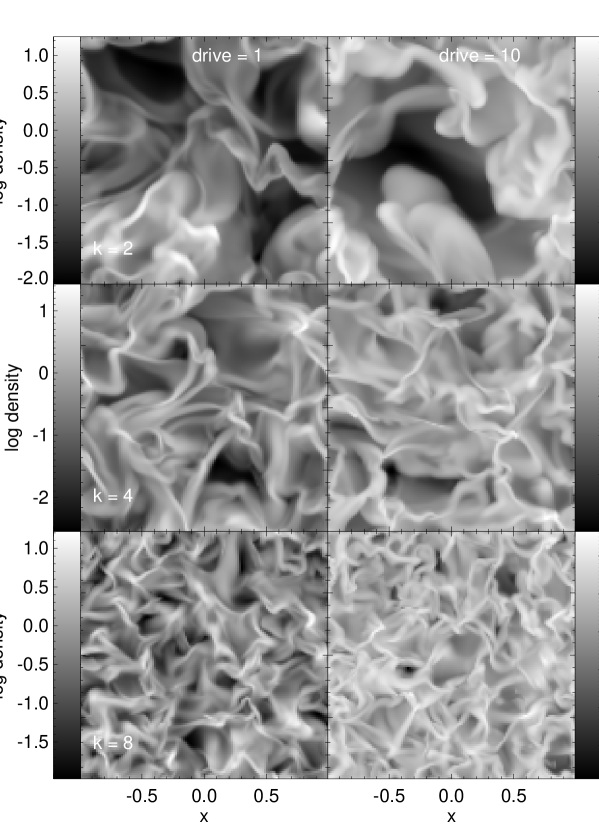
Figure 3: Models showing the appearance of 3D hydrodynamical turbulence driven with dimensionless wavenumber of $k=2$, 4, and 8, and with input energies differing by a factor of 10 (“drive” in the figure. From Mac Low (1999). Figures are scaled to their own maximum and minimum log density.

To measure how strongly equilibrium turbulence dissipated energy, we drove the turbulence with a known, fixed, kinetic energy input rate, $\dot{E}_{K}$, and measured the resulting rms velocity $v$. In the hydrodynamic case, we found that these quantities excellently followed the relation

$$\dot{E}_{K}\simeq(0.21/\pi)m\kappa v^{3}$$ (2)

where $m$ is the mass of the region, and $\kappa=2\pi/\lambda_{D}$ is the dimensionalized wavenumber (for our case, with box-size two, $\kappa=\pi k_{D}$), using $\lambda_{D}$ as the dimensional driving wavelength. Although there is some divergence in the MHD case, this relation is still good to within a factor of two even there.

From this relation, we can compute the decay rate in comparison to the free-fall time $t_{\rm ff}$ of the region (Mac Low 1999). If we make the assumption that $E_{K}=\int\rho(\vec{x})\vec{v}(\vec{x})d\vec{x}\sim(1/2)mv^{2}$ (noting that $v$ is the rms velocity in the region), we can compute a formal decay time $t_{d}=E_{K}/\dot{E}_{K}$ for the turbulence, by substituting in from equations 2 and 1 to find

$$\frac{t_{d}}{t_{\rm ff}}=1.2\pi\frac{\lambda_{D}}{\lambda_{J}}\frac{1}{M},$$ (3)

where $M=v/c_{s}$ is the rms Mach number. Bonnazzola et al. (1987, 1992) have suggested that $\lambda_{D}<\lambda_{J}$ is required for turbulent support to be effective in preventing gravitational collapse; observations show that $M>>1$ in typical molecular clouds (e.g. Blitz 1993), so turbulence appears likely to decay in rather less than a free-fall time, providing no help to explaining the apparent long lives of molecular clouds.

The observed random supersonic motions are likely therefore to be driven. Four energy sources suggest themselves as possible drivers. First, differential rotation of the galactic disk (Fleck 1981) is attractive as it should apply even to clouds without active star formation. Furthermore, support of clouds against collapse by shear could explain the observation that smaller dwarf galaxies, with lower shear, have larger star-formation regions (Hunter 1998). However, the question arises whether this large-scale driver can actually couple efficiently down to molecular cloud scales. Balbus-Hawley instabilities might play a role here (Balbus & Hawley 1998).

Second, turbulence driven by gravitational collapse has the attractive feature of being universal: there is no need for any additional outside energy source, as the supporting turbulence is driven by the collapse process itself. Unfortunately, it has been shown by Klessen, Burkert, & Bate (1998) not to work for gas dynamics in a periodic domain. The turbulence dissipates on the same time scale as collapse occurs, without markedly impeding the collapse. The computations reported below suggest that magnetic fields do not markedly change this conclusion.

Third, ionizing radiation (McKee 1989, Bertoldi & McKee 1997, Vázquez-Semadeni, Passot & Pouquet 1995), winds, and supernovae from massive stars provide another potential source of energy to support molecular clouds. Here the problem may be that they are too destructive, tending rather to destroy the molecular cloud they act on rather than merely stirring it up. If the clouds are coupled to a larger-scale interstellar turbulence driven by massive stars, however, perhaps this problem can be avoided. Ballesteros-Paredes et al. (1999) even suggest that they are both formed and destroyed on short time-scales by this turbulence, a possibility well worth further study.

A final suspect for the driving mechanism is jets and outflows from the common low-mass protostars that should naturally form in any collapsing molecular cloud (McKee 1989, Franco & Cox 1983, Norman & Silk 1980), allowing the attractive possibility of star-formation being a self-limiting process. It has recently become clear that these jets can reach lengths of several parsecs (Bally, Devine, & Alten 1996), implying total energies of order the stellar accretion energy, as suggested by Shu et al. (1988) on theoretical grounds. However, it remains unclear whether space-filling turbulence can be driven by sticking needles into the molecular clouds.

5 Self Gravity

We have begun to investigate directly the support of supersonically turbulent regions against self-gravity by including self-gravity in our models of driven turbulence with and without magnetic fields. Analytic and 2D numerical work by Bonazzola et al. (1987, 1992) and Léorat, Passot, & Pouquet (1990) suggested that a turbulent Jeans wavelength could be defined $\lambda_{J,t}\sim\sqrt{v^{2}/G\rho}$, where $v$ is again the rms velocity in the region. They furthermore specified that the rms velocity differences must be measured at wavenumbers contained in the region in question.

It was already noted by Gammie & Ostriker (1996) in their 1D MHD computations that driving could promote collapse as well as preventing it. We find that this effect is very significant in our 3D models where shocks can intersect at multiple angles. Shocks in isothermal gas compress the gas by a factor of the square of the Mach number, so local densities in a region being supported by supersonic turbulence can exceed the average density by orders of magnitude. The free-fall time and Jeans length drop accordingly in these regions, leaving them no longer supported by the global motions. In Figure 4 we show examples of such collapsed regions in turbulence driven with low and high wavenumbers. The only way to prevent the collapse would be to drive the turbulence at such high power and wavenumber that even regions compressed orders of magnitude above the average were still supported, which appears astrophysically unlikely (driving wavelengths would have to be under $10^{3}$ AU if we take typical molecular cloud parameters for our models). Adding magnetic fields with strengths insufficient to allow magnetostatic support so far appears to make no qualitative difference to these results.

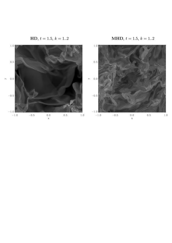
Figure 4: Comparison of slices of log density for turbulently supported hydrodynamic and MHD turbulence computed with ZEUS, approximately one free-fall time after turning on self-gravity. In both cases, small regions have begun to collapse, but most of the gas has not (yet) been accreted by them.

From our preliminary models it appears that global collapse with high star-formation efficiency can be at least strongly delayed, if not prevented, by driven turbulence, but local collapse with low star-formation efficiency will be forced. This leads us to speculate that regions of isolated star formation may correspond to regions supported by supersonic turbulence, while regions of clustered star formation may correspond to regions where the turbulence has been overwhelmed, either by the decay of the local turbulent motions or by the accretion of additional mass due to large-scale flows (e.g. in spiral arms or starburst regions).

- [1] rons, J., & Max, C. E. 1975, ApJ, 196, L77
- [2] allesteros-Paredes, J., Hartmann, L, & Vázquez-Semadeni, E. 1999, ApJ, submitted
- [3] albus, S. A., & Hawley, J. F. 1998, Rev. Mod. Phys., 70, 1
- [4] ally, J., Devine, D., & Alten, V. 1996, ApJ, 473, 921
- [5] enz, W. 1990, in The Numerical Modelling of Nonlinear Stellar Pulsations, ed. J. R. Buchlaer (Kluwer, Dordrecht), 269
- [6] ertoldi, F. B., & McKee, C. F. 1997, Rev. Mex. Astron. Astrophys. Ser. Conf., 6, 195
- [7] litz, L. 1993, in Protostars & Planets III, eds. E. H. Levy & J. I. Lunine (U. of Ariz. Press, Tucson), 125
- [8] litz, L., & Shu, F. H. 1980, ApJ, 238, 148
- [9] onazzola, S. Falgarone, E. Heyvaerts, J. Pérault, M., & Puget, J. L. 1987, A&A, 172, 293
- [10] onazzola, S., Pérault, M., Puget, J. L., Heyvaerts, J., Falgarone, E., & Panis, J. F. 1992, J. Fluid Mech., 245, 1
- [11] larke, D. 1994, NCSA Technical Report
- [12] ranco, J. & Cox, D. P. 1983, ApJ, 273, 24
- [13] leck, R. c., Jr. 1981, ApJ, 246, L151
- [14] ammie, C. F., & Ostriker, E. C. 1996, ApJ, 466, 814
- [15] awley, J. F., & Stone, J. M. 1995, Computer Phys. Comm., 89, 127
- [16] unter, D. 1998, PASP, 109, 937
- [17] lessen, R. S., Burkert, A., & Bate, M. R. 1998, ApJ, 501, L205
- [18] olmogorov, A. N. 1941, Dokl. Acad. Nauk SSSR, 30, 9
- [19] éorat, J., Passot, T., & Pouquet, A. 1990, MNRAS, 243, 293
- [20] ac Low, M-M., Klessen, R. S., Burkert, A., & Smith, M. D. 1998, Phys. Rev. Lett., 80, 2754
- [21] ac Low, M.-M. 1999, ApJ, submitted (astro-ph/9809177)
- [22] ac Low, M.-M., & Ossenkopf, V. 1999, A&A, submitted
- [23] cKee, C. F. 1989, ApJ, 345, 782
- [24] onaghan, J. J. 1992, ARA&A, 30, 543
- [25] akano, T. 1998, ApJ, 494, 587
- [26] orman, C., & Silk, J. 1980, ApJ, 238, 158
- [27] osolowsky, E. W., Goodman, A. A., Wilner, D. J., Williams, J. P. 1999, ApJ, submitted (astro-ph/9903454)
- [28] hu, F. H., Lizano, S., Ruden, S. P., & Najita, J. 1988, ApJ, 328, L19
- [29] tone, J. M., & Norman, M. L. 1992a, ApJS, 80, 753
- [30] tone, J. M., & Norman, M. L. 1992b, ApJS, 80, 791
- [31] tone, J. M., Ostriker, E. C., & Gammie, C. F. 1998, ApJ, 508, 99
- [32] an Leer, B. 1977, J. Comput. Phys. 23, 276
- [33] ázquez-Semadeni, E., Passot, T., & Pouquet, A. 1995, ApJ, 441, 702