The Formation Rate of Blue Stragglers in 47 Tucanae

Abstract

We investigate the effects of changes in the blue straggler formation rate in globular clusters on the blue straggler distribution in the color-magnitude diagram. We find that the blue straggler distribution is highly sensitive to the past formation rate. Comparing our models to new UBV observations of a region close to the core of 47 Tucanae suggests that this cluster may have stopped forming blue straggler formation several Gyr ago. This cessation of formation can be associated with an epoch of primordial binary burning which has been invoked in other clusters to infer the imminence of core collapse.

1 INTRODUCTION

Blue stragglers in globular clusters are thought to be created by stellar mergers. Such mergers can occur in two ways: through the spiraling in and merger of two components of a binary system, or through the direct collision of two stars. The former mechanism is not strongly dependent on cluster density, but the latter occurs more often as the stellar collision rate increases. In a cluster of single stars, the collision rate is a function of cluster density and velocity dispersion (Verbunt & Hut, 1987), but a significant binary population can increase the collision rate well beyond that of a cluster of single stars. The enhanced collisions are caused by resonant encounters with binary stars, which create many more opportunities for the stars involved to collide, thus greatly increasing the collisional cross-section (Leonard, 1989). Thus the formation rate of collisional blue stragglers depends on the current and past cluster density profile, velocity dispersion, and binary population. By studying the number of blue stragglers and their distribution in the color magnitude diagram, we can therefore hope to probe the dynamical history and stellar populations of the cluster.

HST observations of the cores of globular clusters, combined with models of blue straggler formation, have been used to infer global properties of clusters (Bailyn & Pinsonneault, 1995; Sills & Bailyn, 1999; Ouellette & Pritchet, 1998). These studies suggest that blue stragglers in the cores of dense clusters are indeed collisional in origin, and place limits on the binary fraction, mass function, central density, and velocity dispersion of the clusters. Recently, Ferraro et al. (1999) found a remarkably high blue straggler concentration in M80, which was difficult to explain given the relatively low inferred collision rate. A similar situation pertains in M3, although it is less pronounced (Ferraro et al., 1997). Ferraro et al. therefore suggested that M80, and possibly M3, may be in an unusual dynamical state, in which the density has recently become large enough to create a large number of encounters involving primordial binaries, engendering anomalously large collision rates. Such a state may also be required to explain the anomalous, and probably short lived, remnants in the core of NGC 6397 (Cool et al., 1998; Edmonds et al., 1999). The high central density of binaries in NGC 6752 (Rubenstein & Bailyn, 1997) may also imply that the cluster is in an unusual dynamical phase. Once the initial population of primordial binaries has been ”burned”, the collision rate would then be expected to decrease, even as the cluster density continues to rise. Since the primordial binary burning phase is presumably short, it is somewhat disturbing that such a phase has to be invoked at the current time in several different clusters.

In our previous exercises in blue straggler population synthesis, we have assumed approximately constant collision rates. Here, we explore the effects of significant changes in the blue straggler formation rate on the observed distribution of blue stragglers in the color-magnitude diagram. We find that the currently observed blue straggler populations should vary significantly depending on the past formation rate. We apply our results to a new data set from 47 Tuc. The results suggest that this cluster may well have undergone a burst of blue straggler formation which ended several Gyr in the past. In section 2 we present the theoretical models of blue straggler distributions. We discuss the observations of 47 Tuc in section 3, and compare the theory with these observations in section 4. We summarize our findings in section 5.

2 MODELS OF BLUE STRAGGLER DISTRIBUTIONS

We calculate blue straggler distributions in the color-magnitude diagram (hereafter CMD) of 47 Tuc following the method described in detail in Sills & Bailyn (1999). We assume that the blue stragglers are all formed through stellar collisions between single stars during an encounter between a single star and a binary system. The trajectories of the stars during the collision are modeled using the STARLAB software package (McMillan & Hut, 1996). The masses of the stars involved are chosen randomly from a mass function for the current cluster and a different mass function which governs the mass distribution within the binary system. A binary fraction, and a distribution of semi-major axes must also be assumed. The output of these simulations is the probability that a collision between stars of specific masses will occur. We have chosen standard values for the mass functions and binary distribution. The current mass function has an index $x=-2$, and the mass distribution within the binary systems are drawn from a Salpeter mass function ($x=1.35$). We chose a binary fraction of 20% and a binary period distribution which is flat in log P. The effect of changing these values is explored in Sills & Bailyn (1999). The collision products are modeled by entropy ordering of gas from colliding stars (Sills & Lombardi, 1997) and evolved from these initial conditions using the Yale stellar evolution code YREC (Guenther et al., 1992). The models reported here used a metallicity appropriate for 47 Tuc, but the general features we report are similar for any metallicity. By weighting the resulting evolutionary tracks by the probability that the specific collision will occur, we obtain a predicted distribution of blue stragglers in the CMD.

In order to explore the effects of non-constant blue straggler formation rates, we examined a series of truncated rates. In these models we assumed that the blue straggler formation rate was constant for some portion of the cluster lifetime, and zero otherwise. This assumption is obviously unphysical — the relevant encounter rates would presumably change smoothly on timescales comparable to the relaxation time. However these models do demonstrate how the distribution of blue stragglers in the CMD depend on when the blue stragglers were created, and thus provide a basis for understanding more complicated and realistic formation rates.

In Figure 1 we show blue straggler distributions in the CMD for formation rates which were initially zero, and then abruptly “switched on” at some point in the cluster’s past, and continued at a constant rate until the present day. The first panel is the limiting case of constant formation rate throughout the cluster’s lifetime. There are dramatic changes as the onset of blue straggler formation moves closer to the present. In particular, the redder blue stragglers disappear, starting from the faint end, until in Figure 1E the lower part of the blue straggler distribution closely approximates the zero age main sequence (ZAMS).

This behavior is straightforward to interpret. Lower mass blue stragglers start out essentially as ZAMS stars — they are generally formed from low mass precursors which have not processed significant amounts of nuclear fuel, so they have no chemical anomalies. Since their main sequence lifetimes are $>>1$ Gyr, the bottom of the sequence of recently formed blue stragglers closely approximates the ZAMS. In contrast, the more massive blue stragglers evolve much faster, and they are also formed far from the ZAMS in the first place, since their precursors have already undergone considerable nuclear processing. Thus a burst of recent blue straggler formation will create a blue straggler distribution like that in Figure 1E, with a narrow sequence at the low L end, and a relatively large number of stars with a range of temperatures at the bright end.

Figure 2 shows a sequence of blue straggler distributions in which blue straggler formation began at the start of the cluster lifetime, but terminated at some point in the past. The limiting case when the termination point is the present is the same as Figure 1A and has thus been omitted. Figure 2 shows progressively older blue straggler sequences. Once again, the dramatic changes in distribution are easy to understand. The more massive and luminous blue stragglers evolve first, and move away from the ZAMS, and then out of the blue straggler region altogether when they become giants. A population of blue stragglers like that shown in Figure 2d, in which all of the blue stragglers have ages $\geq 8$Gyrs, will therefore contain only relatively faint blue stragglers and will be skewed toward the red away from the ZAMS. The dramatic difference between Figure 1E and Figure 2D, which were created using identical assumptions about binary fraction, mass function, and other dynamical parameters, illustrates the importance of including changes in formation rate in studies of blue straggler distributions. It is difficult to produce such drastic changes in the shape of the blue straggler distribution by varying the mass functions and binary fraction, although these parameters do have a strong influence on the total number of blue stragglers (Sills & Bailyn, 1999).

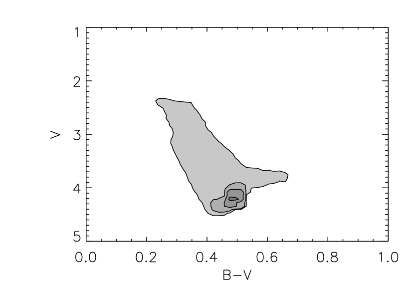
Figure 4: Predicted distributions of blue stragglers in the color-magnitude diagram of 47 Tuc. The blue straggler formation rate is equal to the binary star destruction rate from Hut, McMillan & Romani (1992).

Fig 3 shows distributions of blue stragglers in which the formation rate turned on at some point after the cluster was born, and then turned off again prior to the present. As might be expected, these distributions show characteristics similar to those in both Figs 1 and 2, since both effects described above apply in these cases. We have also used the binary destruction rate from Figure 3 of Hut, McMillan & Romani (1992) as an approximation for blue straggler creation, since both effects result from the same close stellar encounters. The resulting distribution is dominated by old, low luminosity blue stragglers, but also contains a small, but potentially observable population of younger blue stragglers (Figure 4).

3 OBSERVATIONS OF BLUE STRAGGLERS IN 47 TUCANAE

Observations of 47 Tucanae were obtained between July 1996 and January 1997. Data were taken nearly every night for 6 weeks, with some additional coverage over six months with the CTIO 0.9 m telescope and 2K CCD. Repeated UBVI images were obtained for a 13’ $\times$ 13’ field centered on RA,DEC (2000) = 00:22:06.75 -72:04:22.1, with the closest edge 138.5” west of cluster center. The primary purpose was to study variability on the giant branch, and the time series results will be presented elsewhere. In this paper, we present color-magnitude diagrams created from summed data. The exposure times were chosen to avoid saturation of giant branch stars, and are therefore deepest in bluer bandpasses, which makes this data set ideal for studying hot stars, such as blue stragglers. The summed images were analyzed with DAOPHOT and calibrated with Landolt standards. The calibration agrees with that of Hesser et al. (1987) to within 1% for B and V. The stars presented and analyzed in this paper are only those which contribute $>50\%$ of the light within one PSF radius of their centers. This criterion results in the loss of many crowded stars, especially at or below the main sequence turnoff. However the principle sequences derived are quite clean, and the completeness above the turnoff is high, though not 100%. Figure 5 presents the resulting CMD.

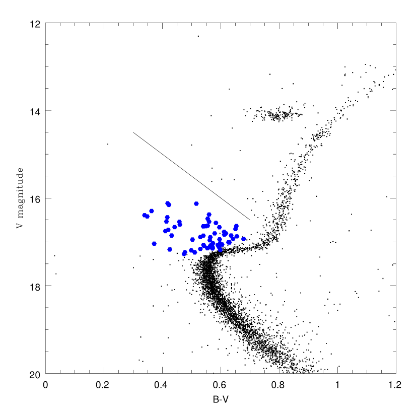
Figure 6: The V vs. B-V color-magnitude diagram for 47 Tucanae. Blue stragglers are constrained to lie below the solid line. The selected sample of blue stragglers is shown as large points.

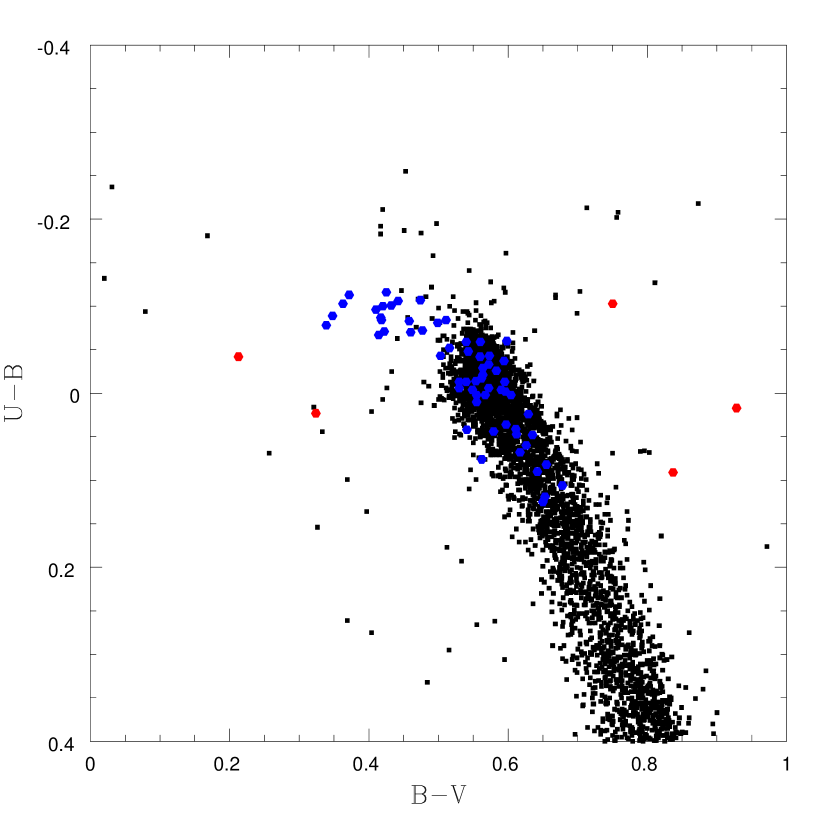
Figure 7: The U-B vs. B-V color-color diagram for 47 Tucanae. The selected sample of blue stragglers is shown as the blue symbols. The 5 red symbols which lie off the principal sequence of the cluster were rejected from the sample.

In order to study the blue stragglers, we must have a consistent way of selecting them from the color-magnitude diagram. It is necessary to make the selection in two colors, since some stars which are present in the blue straggler region in one color may show up as photometric anomalies in other colors. These stars could be foreground or background objects, photometric errors, or other kinds of strange stars which are not blue stragglers. The initial selection was done in the U, U-B diagram (see Figure 5). An additional selection made in V, B-V diagram (see Figure 6), and then stars far from the principle sequence in the color-color diagram were rejected (see Figure 7). Although some of the stars excluded may still be blue stragglers, we have adopted these criteria so that we can have a clean comparison of the data to our theoretical distributions. The star at V$\sim$14.7, B-V$\sim$0.2 and U-B$\sim$-0.05 is known to be a variable star (Edmonds 1999, private communication) and is likely an SX Phoenicis star. However, it does not satisfy our selection criteria, and therefore has been rejected from our sample. Using these criteria, we find 61 blue stragglers (compared to the 20 found by de Marchi, Paresce & Ferraro (1993)). It should be noted that some of the blue stragglers within 0.75 magnitudes above the cluster turnoff could result from the superposition of main sequence stars, either by chance or from being a physical binary. The blue straggler frequency relative to horizontal branch stars (as defined by Ferraro et al. (1999)) is 0.37. We matched our theoretical distributions of BSs to the observations by forming our distributions from those parts of the evolutionary paths which satisfied the above observational selection criteria. We chose to use this data set alone, rather than combining it with the earlier HST data on blue stragglers from the core of the cluster. In order to have a convincing comparison of theory to data, we need a consistent way of selecting the blue stragglers, which can be done best with a large homogeneous data set. In order to understand the properties of 47 Tuc as a whole, eventually data from all sources and all regions of the cluster will have to be considered. The implications of our choice will be discussed in the following section.

4 COMPARISON OF THEORY WITH OBSERVATIONS

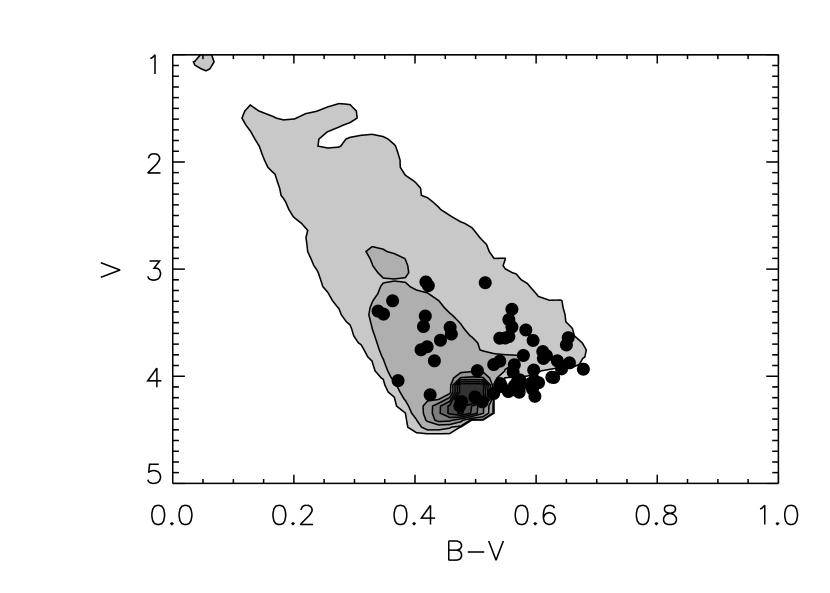
Figure 8: Predicted distribution of blue stragglers in the color-magnitude diagram of 47 Tuc. The blue stragglers were formed at a constant rate throughout the life of the cluster. The solid dots show the observed blue stragglers.

The theoretical blue straggler distribution with a constant blue straggler formation rate is shown in Figure 8, along with the 61 selected blue stragglers. This distribution does not match the observations in three important ways. Firstly, the models predict a large peak of low luminosity blue stragglers which is not observed. This is likely a selection effect, since fainter stars are less likely to pass the 50% contamination test noted above. Secondly, there are too many observed blue stragglers at the red end of the distribution. These so-called “yellow stragglers” have been noted as anomalies before (Stetson, 1994) and may be due to the composite colors of binary stars, or chance superpositions which are fit by only one star in the reduction procedure. Both of these suggestions can be well studied with simulations of the completeness and crowding effects, and will be discussed in a future paper. Thirdly, the theory predicts too many bright blue stragglers. Since the first two problems cannot be addressed in the context of our theoretical models, we focus here on the third point, and explore what is required to produce a theoretical blue straggler distribution which terminates at the same magnitudes as the observed blue stragglers.

As discussed above, the bright blue stragglers have high masses, and do not live very long. Therefore, in order to have a population of blue stragglers which lacks bright stars, the blue stragglers must have stopped forming some time ago. In the context of the models described above, we find that a blue straggler formation rate which terminated 3 Gyr ago reproduces the upper part of the observed blue straggler distribution quite well (Figure 9). However, we caution that the precise date of the termination of blue straggler formation should not be taken too seriously. First, the formation rates used here are not realistic. A full dynamical model of the evolution of the cluster would be required to produce accurate time-dependent rates. Second, our results are influenced by our choice of binary parameters and mass functions, although the same qualitative effects will apply regardless of the choice of these parameters. Third, the observed sample is biased in two important ways. Incompleteness due to crowding will affect the distribution, particularly at the faint end. However this should not affect the lack of bright blue stragglers, which is the observed feature we are trying to reproduce. More importantly, we do not have complete spatial coverage of the cluster. HST results suggest that the blue straggler distribution extends to brighter limits in the cluster core (Gilliland et al., 1998). It is possible that the blue straggler distribution is different in the core because the contribution of blue stragglers created by binary mergers, rather than stellar collisions, is larger in the outer regions. If so, the lack of bright blue stragglers in this region may be more closely related to the characteristics of the binary population in this region than the stellar collision rate. Detailed models of binary merger evolutionary tracks, combined with predictions of the binary population’s merger rate, will be necessary to untangle this degeneracy. The lack of bright blue stragglers outside the core could be explained by mass segregation, either because the more massive blue stragglers sink to the cluster center (although this effect should not be dominant since the mass difference between the bright and faint blue stragglers would be relatively small), or by driving the few remaining binaries toward the center of the cluster. However, we do not believe that mass segregation alone could account for the sharp cutoff in blue straggler luminosities that we observe in the absence of a significant change in the blue straggler formation rate, since it is hard to believe the upper part of the blue straggler distribution could be lost from our observations given that there are large numbers of observed blue stragglers in the $1.1-1.4M_{\sun}$ range.

Thus the data appear to suggest that 47 Tuc has passed through a stage similar to the current state of M80 at some point in the past. The large extent of the blue straggler sequence in M80 observed by Ferraro et al. (1999) tends to support this interpretation, since a cluster whose blue straggler formation rate is unusually high at the present time should tend to appear like that in Figure 1D and 1E. Extending this idea to other clusters, we suggest that the magnitude of the bright end of the blue straggler distribution may be an indicator of when the phase of primordial binary burning occurred in clusters, and may thus correlate with the dynamical properties of the cluster, and the formation rate of other anomalous populations which require stellar encounters (Bailyn, 1995). If this scenario is correct, one might expect that the present binary fraction of 47 Tuc should be substantially lower than those of M80 and M3. The decrease in the binary fraction could be a function of binary properties, such as binary period or mass ratio, since the collisional cross section for binary stars depends on both quantities. The decrease in binary fraction could also be function of radial distance from the core, since we expect that binary stars at the center of the cluster will be destroyed earlier than those further out. Testing these ideas in detail will require construction of complete models of the dynamical history of the relevant clusters, including consideration of the evolution of the binary population, an effort well beyond the scope of this paper.

5 SUMMARY

We find that changes in the past formation rate of blue stragglers produces drastic changes in their observed distribution in the CMD. A comparison between our parameterized models and observed blue stragglers in 47 Tuc suggest that this cluster may have undergone an epoch of enhanced BS formation several Gyrs ago. We associate this enhanced blue straggler formation rate with the epoch of primordial binary burning invoked to explain the current characteristics of several other clusters. Since this epoch may well be short, it is reassuring to find a cluster which has evidently gone through this stage in the past, rather than experiencing it currently. Much more detailed dynamical models will be required to explore whether the primordial burning scenario is consistent with the observed blue straggler sequences in globular clusters.

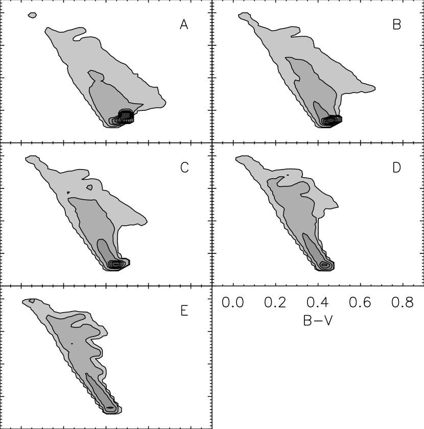
Figure 1: Blue straggler distributions in the color magnitude diagram. The contours represent density levels of stars per magnitude bin, with darker colors corresponding to higher density. The blue straggler formation rate is assumed to be constant, and lasting from some time in the past to the current day. Panel A is the distribution which results if blue stragglers are formed throughout the life of the cluster. The blue straggler formation began 8 Gyr ago in panel B, 5 Gyr ago in panel C, 2 Gyr ago in panel D and 1 Gyr ago in panel E. The contour levels are 0.1,1,5,10,15,20 and 25 blue stragglers per 0.012 magnitudes².

Figure 2: Blue straggler distributions in the color magnitude diagram. The blue straggler formation rate is assumed to be constant, starting at the birth of the cluster, and ending some time in the past: 1 Gyr ago (panel A), 2 Gyr ago (panel B), 5 Gyr ago (panel C) or 8 Gyr ago (panel D).

Figure 3: Blue straggler distributions in the color magnitude diagram. The blue straggler formation rate is assumed to be constant between 2 and 5 Gyr ago (panel A), or between 1 and 2 Gyr ago (panel B).

Figure 5: The U vs. U-B color-magnitude diagram for 47 Tucanae, showing all 4695 stars which contribute more than 50% of the light within 1 PSF radius. The box shows the first selection criterion for blue stragglers.

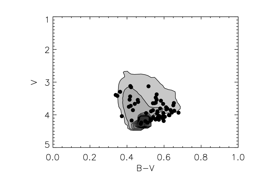
Figure 9: Predicted distributions of blue stragglers in the color-magnitude diagram of 47 Tuc. The blue stragglers were formed at a constant rate until 3 Gyr ago, and no blue stragglers were formed after that.

References

- Bailyn (1995) Bailyn, C. D. 1995, ARA&A, 33, 133
- Bailyn & Pinsonneault (1995) Bailyn, C. D. & Pinsonneault, M. H. 1995, ApJ, 439, 705
- Cool et al. (1998) Cool, A., Grindlay, J. E., Cohn, H. N., Lugger, P., Bailyn, C. D. 1998, ApJ, 508, 75
- de Marchi, Paresce & Ferraro (1993) de Marchi, G., Paresce, F., Ferraro, F. R. 1993, ApJS, 85, 293
- Edmonds et al. (1999) Edmonds, P., Grindlay, J. E., Cool, A., Cohn, H., Lugger, P., Bailyn, C. D. 1999, ApJ, 516, 250
- Ferraro et al. (1997) Ferraro, F., Paltrinieri, B., Fusi Pecci, F., Cacciari, C., Dorman , B., Rood, R. T., Buonanno, R., Corsi, C. E., Burgarella, D., Laget, M. 1997, aap, 324, 915
- Ferraro et al. (1999) Ferraro, F.R., Paltrinieri, B., Rood, R. T., Dorman, B. 1999, ApJ, 522, 983
- Gilliland et al. (1998) Gilliland, R. L., Bono, G., Edmonds, P. D., Caputo, F., Cassisi, S., Petro, L. D., Saha, A., & Shara, M. M. 1998, ApJ, 507, 818
- Guenther et al. (1992) Guenther, D. B., Demarque, P., Kim, Y.-C., & Pinsonneault, M. H., 1992 ApJ, 387, 372
- Hesser et al. (1987) Hesser, J. E., Harris, W. E., Vandenberg, D. A., Allwright, J. W., Shott, P., Stetson, P. B. 1987, PASP, 99, 739
- Hut, McMillan & Romani (1992) Hut, P., McMillan, S., & Romani, R. W. 1992, ApJ, 389, 527
- Leonard (1989) Leonard, P. J. T. 1989, AJ, 98, 217
- McMillan & Hut (1996) McMillan, S. L. W., & Hut, P. 1996, ApJ, 467, 348
- Ouellette & Pritchet (1998) Ouellette, J. A., & Pritchet, C. J. 1998, AJ, 115, 2539
- Rubenstein & Bailyn (1997) Rubenstein, E., & Bailyn, C. D. 1999, ApJ, 474, 701
- Sills & Lombardi (1997) Sills, A. & Lombardi, J. C., Jr. 1997, ApJ, 489, L51
- Sills & Bailyn (1999) Sills, A., & Bailyn, C. D. 1999, ApJ, 513, 428
- Stetson (1994) Stetson, P. B. 1994, PASP, 106, 250
- Verbunt & Hut (1987) Verbunt, F., & Hut, P. 1987,