Redshifts and age of stellar systems of distant radio galaxies from multicolour photometry data

Abstract

Using all the data available in the literature on colour characteristics of host galaxies associated with distant (z$>$1) radio galaxies, a possibility has been investigated of using two evolutionary models of stellar systems (PEGASE and Poggianti) to evaluate readshifts and ages of stellar systems in these galaxies. Recommendations for their applications are given.

Key words:   radio continuum: galaxies - galaxies: distances and redshifts - galaxies: fundamental parameters

1 Introduction

The labour intensity of obtaining statistically significant high-quality data on distant and faint galaxies and radio galaxies forces one to look for simple indirect procedures in the determination of redshifts and other characteristics of these objects. With regard to radio galaxies, even photometric estimates turned out to be helpful and have so far been used (McCarthy, 1993; Benn et al., 1989).

In the late 1980s and early 1990s it was shown that the colour characteristics of galaxies can yield also the estimates of redshifts and ages for the stellar systems of the host galaxies. Numerous evolutionary models appeared with which observational data were compared to yield results strongly distinguished from one another (Arimoto and Yoshii, 1987; Chambers and Charlot, 1990; Lilly, 1987, 1990).

Over the last few years the two models: PEGASE (Project de’Etude des Galaxies par Synthese Evolutive (Fioc and Rocca-Volmerange, 1997)) and Poggianti (1997) have been extensively used, in which an attempt has been made to eliminate the shortcomings of the previous versions.

In the “Big Trio” experiment (Parijskij et al., 1996) we also attempted to apply these techniques to distant objects of the RC catalogue with ultrasteep spectra (USS). Colour data for nearly the whole basic sample of USS FR II (Fanaroff and Riley, 1974) RC objects have been obtained with the 6 m telescope of SAO RAS. In the present paper we investigate the applicability of new models to the population of all distant ($z>1$) radio galaxies with known redshifts. The results of this investigation will be used for the RC objects of the “Big Trio” project.

2 Data

To test the potentialities of the method in determination of the redshifts and ages of the stellar population in the host galaxies from photometry data, we have selected about 40 distant radio galaxies with known redshifts, for which the stellar magnitudes in more than 3 bands are available in the literature (Parijskij et al., 1997). The data on these objects are tabulated in Table 1, in the columns of which are listed the universally accepted names of the sources, IAU names, spectroscopic redshifts (z_sp), apparent stellar magnitudes in the filters from U to K, radio morphology of the objects (P — point source, D — double, T — triple, Ext — extended), and notes. The bracketed values or the values representing the lower limits were disregarded in the calculations. Magnitudes from R column which have a symbol “r” (r-filter) in further calculations were decreased by 0.35 to be used as R magnitudes. Magnitudes from I column with the symbol “i” were decreased by 0.75 and treated as I magnitudes.

The lines describing the objects 3C 65 (B022036+394717), 3C 68.2 (B023124+312110), 3C 184 (B073359+703001) contain the data in which the authors have already taken into account the absorption.

The asterisks in the notes mark the classical FR II-type objects.

It should be noted that the photometry data presented in Table 1 are rather inhomogeneous, obtained using different tools with different apertures and by different observers.

The procedure of estimating the redshifts and ages of the stellar population for each source consisted in:

1. Obtaining the age of the stellar population of the host galaxies from photometry data, PEGASE and Poggianti models with a fixed known redshift.

2. Searching for an optimal model of an object and simultaneous searching for the redshift and age of the stellar population.

3. Comparing the derived values.

3 Description of models of energy distribution in the spectra of the host galaxies

The new model PEGASE (Fioc and Rocca-Volmerange, 1997) for the Hubble sequence galaxies, both with star formation and evolved, was used as a basic SED (Spectral Energy Distribution) model. The uniqueness of this model consists in expanding to the near IR (NIR) of Rocca-Volmerange and Guiderdoni’s (1988) atlas of synthetic spectra with a revised stellar library, which includes parameters of cool stars. The NIR is connected coherently with the visible and ultraviolet ranges, so the model is continuous and spans a range from 220 Å  to 5 microns. The precise algorithm of the model, to quote the authors, allows revealing rapid evolutionary phases such as red supergiants or AGB in the NIR.

We used from this model a wide collection of SED curves from the range of ages between $7\cdot 10^{6}$ and $19\cdot 10^{9}$ years for massive elliptical galaxies.

A second model, taken from Poggianti (1997), is based on computations that include the emission of the stellar component after Barabaro and Olivi (1991), synthesizes the SED for galaxies in the spectral range 1000–10000 Å  and includes the computed phases of stellar evolution for AGB and Post-AGB along with the main sequence and helium burning phase. The model allows for the chemical evolution in the galaxy and therefore for the contribution of the stellar populations of different metallicities to the integral spectrum. Using the stellar model atmospheres (Kurutz, 1992) Poggianti has managed to compute spectrum up to 25000 Å. Kurutz’s model for stars with ${\rm T_{eff}>5500K}$ has been used in the IR range, while for lower effective temperatures the library of the observed stellar spectra (Lancon and Rocca-Volmerange, 1992) has been employed.

From the second model we have used the SED curves computed for elliptical galaxies, for the ages (2.2, 3.4, 4.3, 5.9, 7.4, 8.7, 10.6, 13.2, 15)$\cdot 10^{9}$ years.

4 Procedure

4.1 Allowance for the absorption

In order to take account of the absorption, we have applied the maps (as FITS-files) from the paper “Maps of Dust IR Emission for Use in Estimation of Reddening and CMBR Foregrounds” (Schlegel et al., 1998). The conversion of stellar magnitudes to flux densities has been performed by the formula (e.g. von Hoerner, 1974):

$$S(Jy)=10^{C-0.4m}.$$

The values of the constant $C$ for different bands are given in Table 2 where also are presented the following characteristics: filter name, wavelength, coefficient A/E(B–V) of transition from distribution of dust emission to absorption in a given band, assuming the absorption curve $R_{V}=3.1$.

Table 2: Properties of bands used in this research

Filter name	$\lambda_{eff}$	A/E(B-V)	C
Landolt U	3600	5.434	3.280
Landolt B	4400	4.315	3.620
Landolt V	5500	3.315	3.564
Landolt R	6500	2.673	3.487
Landolt I	8000	1.940	3.388
UKIRT J	12000	0.902	3.214
UKIRT H	16500	0.576	3.021
UKIRT K	22000	0.367	2.815

The coordinates of sources for the epoch 1950.0, galactic coordinates, and also the absorptions adopted in the further computations are tabulated in Table 3.

4.2 Fitting

The estimation of ages and redshifts was performed by way of selection of the optimum location on the SED curves of the measured photometric points obtained when observing radio galaxies in different filters. We used the already computed table SED curves for different ages. The algorithm of selection of the optimum location of points on the curve consisted briefly (for details see Verkhodanov, 1996) in the following: by shifting the points lengthwise and transverse the SED curve such a location was to be found at which the sum of the squares of the discrepancies was a minimum. Through moving over wavelengths and flux density along the SED curve we estimated the displacements of the points from the location of the given filter and then the best fitted positions were used to compute the redshift. From the whole collection of curves, we selected the ones on which the sum of the squares of the discrepancies turned out to be minimal for the given observations of radio galaxies.

Thus we estimated both the age of the galaxy and the redshift within the frame of the given models (see also Verkhodanov et al., 1998a,b). When apprizing the robustness of fitting, the presence of points from infrared wavelengths (up to the K range) is essential, since in the  fitting we include the  jump before  the

infrared region of the SED and can thus locate stably (with a well-defined maximum on the likelihood curve) our data. When removing the points available (to check the robustness) and leaving only 3 points (one of which is in the K range), we obtain in the fitting the same result on the curve of discrepancies as for 4 or 5 points. If the infrared range is not used, the result proves to be more uncertain.

The computation results with the fixed redshift value are given in Table 4, where there listed 1) the name of the object, 2) the spectroscopic redshift, $z_{sp}$, 3) the age estimated from Poggianti’s models with $z_{sp}$, 4) the r.m.s. deviation, $\sigma_{d}$, of photometric points (Jy) from the optimum age SED curve in Poggianti’s model, 5) the age determined from the PEGASE library models with $z_{sp}$, 6) the r.m.s. deviation, $\sigma_{d}$, of photometric points (Jy) from the optimum age SED curve in the PEGASE model. Note that in the cases where we fail to find a consistent solution, the parameters being determined are omitted in Tables 4 and 5.

Figures 9–54 (at the end of the paper) represent the optimum (with a minimum of the squares of the deviations) SED curves with the given spectroscopic $z_{sp}$ for the sources under investigation and the curves of the dependence of r. m. s. deviations on age for the given object for both models. The pictures are drawn in pairs “SED–$\sigma_{d}$(age)” for the models of Poggianti and PEGASE, respectively. The figures from the SED models of Poggianti and PEGASE are denoted by (a) and (b), respectively.

The result of computations of the redshifts and the age of the stellar population of the host galaxy from the models of PEGASE and Poggianti are tabulated in Table 5 which presents 1) the object name, 2) the spectroscopic redshift, $z_{sp}$, 3) the age estimated from Poggianti’s models in the case of uncertain redshift, 4) the redshift estimate in these models, 5) the r. m. s. deviation, $\sigma_{d}$, of photometric points from the optimum age SED curve in Poggianti’s model for the given case, 6) the age determined from the PEGASE library models in the case of non-fixed redshift, 7) the r. m. s. deviation, $\sigma_{d}$, of photometric points from the optimum age SED curve in the PEGASE model for the given case.

In Figures 55–100 (at the end of the paper) are presented the optimum (with a minimum of the squares of the deviations) SED curves with a variable redshift and normalized likelihood function (LHF) distributions in the “redshift–age” plane for the given object for the two models. The pictures are drawn in pairs “SED–LH function (z, age)” for Poggianti’s and PEGASE models, respectively. When there are several selected curves within one model, all the versions are presented. When it is impossible to choose a model, only the LHF distribution is given. The LHF contours are plotted in the figures by levels 0.6, 0.7, 0.9 and 0.97. The figures from the SED models of Poggianti and PEGASE are labeled by symbols (a) and (b), respectively.

Table 4: Estimated ages at fixed $z$ for studied radio galaxies for Poggianti and PEGASE models

		Poggianti		PEGASE
Object	$z_{sp}$	Age,	$\sigma_{d}$	Age,	$\sigma_{d}$
		Gyr		Gyr
B001151$-$022236	2.08	4.3	0.104	2.00	0.076
B003133$+$390745	1.35	3.4	0.081	1.60	0.052
B015615$-$251404	2.09	7.4	0.100	9.00	0.197
B022036$+$394717	1.176	5.9	0.092	9.00	0.092
B023124$+$312110	1.575	4.3	0.112	3.50	0.067
B031602$-$254603	3.142	4.3	0.049	1.40	0.043
B040644$-$242606	2.427	$\leq$2.2	0.056	0.70	0.024
B050825$+$602718	3.791	$\leq$2.2	0.282	0.25	0.220
B064720$+$413404	3.8	$\leq$2.2	0.046	0.60	0.036
B073359$+$703001	0.994	5.9	0.035	4.50	0.046
B080637$+$423657	1.185	4.3	0.111	2.00	0.121
B083456$-$194114	1.032	$\leq$2.2	0.905
B090224$+$341958	3.395	3.4	0.146	1.40	0.156
B100839$+$464309	1.781	3.4	0.197	1.00	0.155
B101744$+$371209	1.05	$\leq$2.2	0.057	0.70	0.022
B101909$+$221439	1.617	4.3	0.084	2.00	0.069
B105623$+$394106	2.171	4.3	0.044	2.50	0.031
B110643$+$380047	2.29	5.9	0.208	2.50	0.183
B110847$+$355703	1.105	$\leq$2.2	0.091	0.80	0.102
B111347$+$345847	2.40	4.3	0.292	1.80	0.258
B113226$+$372516	2.88	5.9	0.295	3.00	0.355
B114304$+$500248	1.275	$\leq$2.2	0.104	0.60	0.020
B114722$+$130400	1.142	3.4	0.072	1.80	0.039
B115920$+$365136	2.78	7.4	0.323	8.00	0.377
B122954$+$262040	2.609	$\leq$2.2	0.087	0.70	0.039
B123239$+$394209	3.225	4.3	0.227	3.00	0.273
B125440$+$473632	0.996	4.3	0.070	2.50	0.070
B125649$+$353605	1.13	5.9	0.048	6.00	0.046
B134554$+$243046	2.889	3.4	0.046	1.00	0.072
B140434$+$342540	1.779	4.3	0.123	2.50	0.173
B141607$+$524318	0.992	$\leq$2.2	0.085	1.00	0.010
B154737$+$213441	1.207	$\leq$2.2	0.054	0.90	0.051
B171259$+$501851	2.387	$\leq$2.2	0.138	0.70	0.100
B172117$+$500848	1.55	5.9	0.096	8.00	0.129
B172307$+$510015	1.079	$\leq$2.2	0.047	0.90	0.057
B175921$+$135122	1.45	4.3	0.042	1.80	0.040
B180245$+$110115	1.132	$\leq$2.2	0.080	0.80	0.066
B180919$+$404439	2.267	5.9	0.185	3.00	0.171
				4.50	0.171
B193140$+$480509	2.348	4.3	0.174	1.20	0.145
B202504$-$215055	2.63	$\leq$2.2	0.083	0.80	0.065
B210500$+$231938	2.479	$\leq$2.2	0.063	0.70	0.050
B214501$+$150641	1.48	3.4	0.071	1.60	0.011
B220430$-$201808	1.62	4.3	0.080	1.80	0.034
B224858$+$711324	1.841	$\leq$2.2	0.069	0.80	0.067
B234927$+$285348	2.905	4.3	0.111	4.50	0.052
B235332$-$014833	1.028	3.4	0.057	1.60	0.029

Table 5: Estimated ages and $z$ for the studied radio galaxies for Poggianti and PEGASE models in assumption of unknown $z$

		Poggianti			PEGASE
Object	$z_{sp}$	Age,	$z_{e}st$	$\sigma_{d}$	Age,	$z_{e}st$	$\sigma_{d}$
		Gyr			Gyr
B001151$-$022236	2.08	4.3	1.11	0.003	1.40	2.64	0.009
					2.50	3.27	0.003
B003133$+$390745	1.35	7.4	0.64	0.038	1.60	1.54	0.029
B015615$-$251404	2.09	7.4	1.91	0.033
B022036$+$394717	1.176	5.9	1.11	0.090	9.00	1.17	0.079
B023124$+$312110	1.575	4.3	1.33	0.084	3.00	1.37	0.049
					1.00	0.82	0.039
B031602$-$254603	3.142	4.3	3.52	0.014	1.40	2.64	0.000
B040644$-$242606	2.427	4.3	0.50	0.027	0.70	1.86	0.016
					1.00	0.80	0.013
B050825$+$602718	3.791	4.3	0.04	0.142
B064720$+$413404	3.8	3.4	4.35	0.003	0.60	4.20	0.019
B073359$+$703001	0.994	4.3	1.11	0.024	3.00	1.04	0.010
		5.9	0.98	0.025	6.00	0.86	0.021
B080637$+$423657	1.185	4.3	1.91	0.063	2.00	2.07	0.055
B083456$-$194114	1.032	$\leq$2.2	4.06	0.585
B090224$+$341958	3.395	4.3	3.52	0.038	1.40	4.19	0.119
B100839$+$464309	1.781	4.3	0.65	0.064	1.80	0.86	0.052
B101744$+$371209	1.05	8.7	0.11	0.004	0.45	4.39	0.008
					5.00	0.21	0.002
B101909$+$221439	1.617	4.3	1.57	0.077	2.00	1.59	0.065
B105623$+$394106	2.171	5.9	4.06	0.011	4.00	2.53	0.003
					8.00	3.44	0.003
					1.00	3.82	0.004
B110643$+$380047	2.29	4.3	1.30	0.055	3.00	1.47	0.012
B110847$+$355703	1.105	3.4	3.04	0.060	1.00	3.37	0.019
					2.50	4.56	0.018
B111347$+$345847	2.40	4.3	1.23	0.067	3.00	1.08	0.058
B113226$+$372516	2.88	5.9	1.09	0.048	9.00	1.08	0.009
B114304$+$500248	1.275	$\leq$2.2	3.48	0.019	0.60	2.59	0.003
		4.3	0.25	0.021	0.80	0.74	0.001
					4.50	0.22	0.009
B114722$+$130400	1.142	5.9	0.64	0.042	1.60	1.17	0.029
B115920$+$365136	2.78	5.9	1.67	0.113
B122954$+$262040	2.609	$\leq$2.2	2.64	0.065	0.70	2.61	0.023
B123239$+$394209	3.225	4.3	1.06	0.098	1.80	3.73	0.093
B125440$+$473632	0.996	5.9	0.64	0.046	4.50	0.70	0.051
B125649$+$353605	1.13	7.4	1.05	0.041	6.00	1.12	0.018
B134554$+$243046	2.889	3.4	2.71	0.042	1.00	2.31	0.031
B140434$+$342540	1.779	8.7	1.96	0.005	2.00	2.36	0.005
B141607$+$524318	0.992	4.3	0.39	0.044	1.00	1.00	0.000
B154737$+$213441	1.207	$\leq$2.2	1.51	0.033	0.70	5.99	0.022
B171259$+$501851	2.387	$\leq$2.2	0.65	0.073	0.60	2.05	0.051
B172117$+$500848	1.55	5.9	1.28	0.046	2.00	1.17	0.048
B172307$+$510015	1.079	$\leq$2.2	1.49	0.021	0.90	3.14	0.014
B175921$+$135122	1.45	4.3	2.62	0.013	1.80	2.62	0.006
					3.00	3.36	0.006
B180245$+$110115	1.132	$\leq$2.2	0.97	0.078	0.80	1.17	0.055
B180919$+$404439	2.267	4.3	1.98	0.102	2.50	1.96	0.065
B193140$+$480509	2.348	3.4	1.98	0.100	1.40	1.95	0.020
B202504$-$215055	2.63	$\leq$2.2	2.19	0.047	0.80	2.39	0.028
B210500$+$231938	2.479	3.4	3.52	0.026	0.60	4.19	0.032
B214501$+$150641	1.48	7.4	0.64	0.006	1.60	1.60	0.001
B220430$-$201808	1.62	4.3	2.62	0.010	1.80	2.62	0.004
					3.50	3.36	0.004
B224858$+$711324	1.841	$\leq$2.2	1.11	0.025	0.90	2.07	0.035
		8.7	0.26	0.024
B234927$+$285348	2.905	5.9	3.95	0.020	6.00	3.17	0.006
B235332$-$014833	1.028	3.4	0.86	0.036	1.60	1.10	0.001

Note that the sought-for parameters for 11 sources are determined ambiguously.

5 Discussion

The principal points of our concern are:

• whether one can use the multicolour photometry technique to measure the redshift (first of all) and age of the stellar population of the host galaxy for distant radio galaxies;

• which of the new models give the best agreement of the redshift found by spectroscopy with the derived values;

• to what extent one can rely on the obtained ages of radio galaxies.

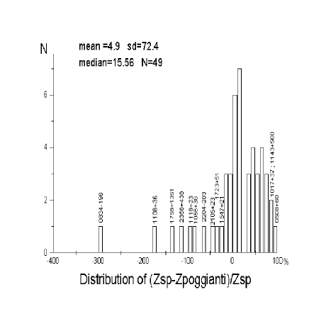
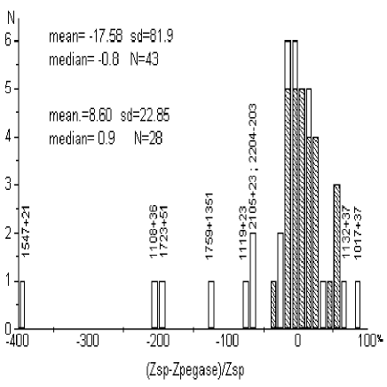
Figure 1: The histogram of distribution of the normalized difference (in percent) of the redshift (spectral, $z_{sp}$) and the redshift obtained from the SED models: (a) for Poggianti’s models, (b) for PEGASE models. The shaded columns in Fig. 1b represent the sample of classical FR II objects marked with an asterisk in Tables 1, 5. The object 1547+21 is a gravitational lens, the redshift estimates for the objects 1108+36 and 1017+37 do not conform to possible photometric redsift limits, this is why they must be excluded from the discussion; the object 1119+25 is N galaxy; the radio source 1132+37 has a GPS spectrum.

Should all the data of Table 5 be used with no selection (leaving only one of the versions for each object), the formal error of one measure of the redshift equals 70–80 % (Fig. 1 a, b), which is almost an order of magnitude worse than for nearby objects (see e. g. Benn et al., 1989). For Poggianti’s models residuals are less clustered in their distribution (compare Fig. 1 a and 1 b).

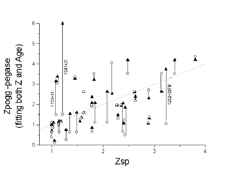
Figure 2: The relationship between PEGASE and Poggianti model redshifts and spectral redshift. The data for one and the same source are joined by the vertical lines. The triangles are for the PEGASE models, the circles are for Poggianti’s. The names of the sources are given in cases where the difference between the models is large. $Y=X$ is represented by the dotted line.

The situation improves considerably if Table 5 is restricted only by the population of classical FRİI-type objects (marked by asterisks in Tables 1, 5). For the PEGASE models the error decreases to 23 %. It is essential that this error has not been revealed to rise with $z_{sp}$ (Fig. 2). Part of the error is without a doubt associated with quality and dissimilarity of observational data, part with the real difference between the SEDs of host galaxies and adopted models.

In a number of properties the PEGASE models turn out to be closer to the real SED for radio galaxies than Poggianti’s models. This is why it is conceived to employ the former for distant FR II-type galaxies until models of higher quality appear.

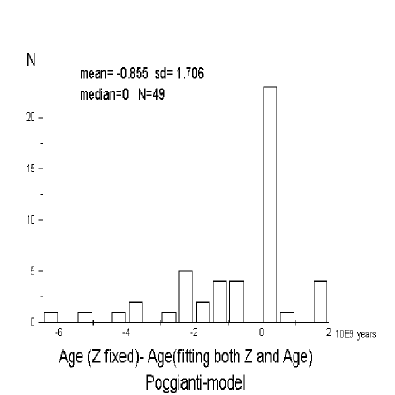
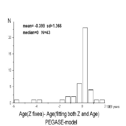
Figure 3: The distribution of the difference in the ages obtained when computing with $z_{sp}$ and when selecting both parameters simultaneously for Poggianti’s and PEGASE models, (a) and (b), respectively.

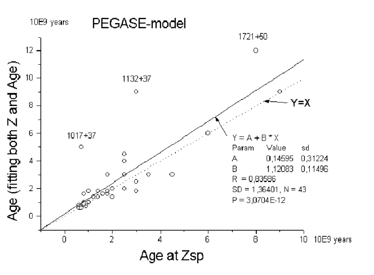
Figure 4: Comparison of the ages of stellar population of the host galaxy obtained from the PEGASE models in different ways. The ordinate is the age when searching for redshift and age simultaneously. The age with a fixed known spectral redshift is plotted on an abscissa. The straight solid line is the linear regression, the dotted line is the $Y=X$ line. For the highly “sallied out” points, the names of the sources are indicated.

The errors in age estimates of the stellar population from the data of Tables 4 and 5 can so far be determined only by comparing results of different models, which may not represent the true error. Histograms of such “model” errors in age determination of the stellar population of host galaxies are displayed in Fig. 3a, b. The ages derived from the PEGASE models with a fixed (spectroscopic) redshifts are generally little (10 %) different from the version of simultaneous selection of both age and redshift (Fig. 4).

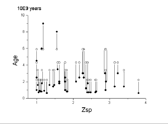
Figure 5: The age of the stellar population of the host galaxy (with a fixed $z$) vs. the redshift for PEGASE (filled circles), Poggianti (open circles). The data for one and the same source are joined by the vertical lines.

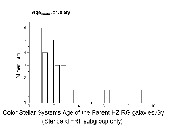
Figure 6: The histograms of the age distribution of the host galaxy stellar population from the PEGASE models for the subsample of radio galaxies of FR II type (in Tables 1 and 5 these objects are marked with the asterisks).

Fig. 5 shows the differences in age from the models of Poggianti and PEGASE, depending on the spectroscopic redshift. The average age of radio galaxies turned out to be about 2 billion years (see e. g. Fig. 6) and only slightly depends on $z_{sp}$. The dispersion of age values decreases with growing $z_{sp}$, though the statistical significance of this inference is not high. Besides, there is a systematic difference in the ages estimated from these two models. Poggianti’s model yields a larger by about 1.5–2 billion years age value, except for the utmost ages. Note that the larger the age, the lower its estimation accuracy. For the oldest systems, the differences in the ages estimated from the two models may amount to 100 % and above.

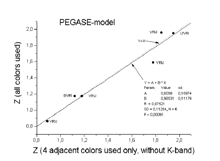
Figure 7: The redshift derived from all the data available, including K bands, (see Table 5) against that obtained with the use of only four adjacent bands, which cover continuously a certain spectrum region. The bands used in the computation (Table 6) are indicated. The solid line is the linear regression, the dotted line is the $Y=X$ line.

The part played by the red filters, especially K, grows with increasing $z$, but it turns out that the “continuity” in the location of the filters across the determined spectrum region is essential. To illustrate this we have compared the accuracy of determination of colour redshifts in two cases: using all the data available, including the K filter and with the application of four neighbouring filters that cover continuously a specified region of the spectrum. We have managed to select 6 of such cases (Tables 6 and 7), and all of them are used in Fig. 7. It follows from the figure that the difference in colour redshifts is as small as 11 %. This allows us to hope for being able to estimate colour redshifts with a sufficient accuracy by using the standard equipment available at SAO RAS.

In selecting the most likely version of colour redshift one can use photometry data in a separate filter since the difference between these versions exceeds sometimes the errors in photometric estimates (see e. g. objects 1108+38, 1017+37).

Using the age of stellar systems of the host galaxies, one can roughly evaluate the time of the latest mass star formation T_sf and the redshift $z_{sf}$, corresponding to that moment. These estimates are model dependent and we restrict ourselves to the standard CDM model of the Universe.

Table 6: Estimated ages at fixed $z$ for studied radio galaxies for Poggianti and PEGASE models for selected filters

		Poggianti		PEGASE
IAU name	$z_{sp}$	Age,	$\sigma_{d}$	Age,	$\sigma_{d}$	Used
		Gyr		Gyr		bands
B022036$+$394717	1.176	5.9	0.055	$\geq$19.0	0.040	BVRI
B100839$+$464309	1.781	4.3	0.135	2.0	0.113	VRIJ
B101909$+$221439	1.617	4.3	0.076	3.5	0.042	VRIJ
B172117$+$500848	1.55	5.9	0.106	$\geq$19.0	0.143	VRIJ
B180919$+$404439	2.267	5.9	0.071	$\geq$19.0	0.093	VRIJ
B193140$+$480509	2.348	8.7	0.119	1.0	0.156	UVRI

Table 7: Estimated ages and $z$ for studied radio galaxies for Poggianti and PEGASE models in assumption of unknown $z$ using selected filters

		Poggianti			PEGASE
Object	$z_{sp}$	Age,	$z_{e}st$	$\sigma_{d}$	Age,	$z_{e}st$	$\sigma_{d}$
		Gyr			Gyr
B022036$+$394717	1.176	5.9	1.29	0.043	$\geq$19.00	1.12	0.027
B100839$+$464309	1.781	4.3	0.89	0.028	2.50	0.89	0.022
		7.4	2.84	0.024
B101909$+$221439	1.617	10.6	3.73	0.022	7.00	1.78	0.009
B172117$+$500848	1.55	7.4	1.46	0.014	$\geq$19.00	1.18	0.017
B180919$+$404439	2.267	5.9	2.08	0.038	3.00	1.85	0.037
		10.6	4.18	0.045
		15.0	3.84	0.043
B193140$+$480509	2.348	4.3	1.98	0.082	1.20	1.95	0.017

The distribution of T_sf for the FR subsample is displayed in Fig. 8. For the average $z_{sf}$ of this sample, the mean age of stellar systems of host galaxies equals 1.8 billion years, which corresponds to $z_{sf}=5.5\pm 3.7$. A considerable part of galaxies have $z_{sf}$ larger than 8, which is important for the reconstruction of the history of the Universe. The presence of a certain number of “negative” ages may be due to the error in age estimates of old objects. The well-studied “negative”-age object 53W091, having $z_{sf}=1.55$ and age of 3.5–4 billion years, has been found to conflict with the CDM model. The conflict can readily be resolved by introduction of the $\Lambda$ term (Dunlop et al., 1996; Krauss, 1997). In any event it is vital that the mean epoch of mass star formation for a population of galaxies with $z>1$ occurs much earlier than, on average, for field galaxies (Cowie et al., 1995).

6 Conclusions

1. It is shown that one can measure redshifts with an accuracy of 25–30 % up to the limiting values for 40 radio galaxies with $1<z<4$, having measured stellar magnitudes in more than 3 filters. These measures are valid first of all for the PEGASE models of SED evolution with time. Therefore it is hoped we will succeed in obtaining sufficiently reliable redshifts from the 6 m telescope multicolour photometry data, using the PEGASE models for the sample of the “Big Trio” project RC objects, though we have no measurements in the K filter. Thus we have obtained good agreement between spectral and colour redshifts for one of the distant RC objects (Dodonov et al., 1999).

2. Ages and moments of the latest vigorous star formation have been estimated for the radio galaxies with $z>1$ discussed above. Stellar population of most objects of this sample is not too old (median PEGASE model age is 1.5 billion years). The age of the stellar population from the models of Poggianti is by 2–2.5 billion years greater. There is not a single object having an age over 7–12 billion years. No perceptible relationship between the age of the stellar population and redshift is observed.

3. The errors can be distinguished as rough ones, that are introduced by the quasiperiodic SED structure, and random errors, which are due to the quality of observational data. The former may reach 100 %, the latter 5–10 %. Simple photometric redshift evaluations allow false estimate to be discarded in a number of cases.

4. A better insight into evolutionary tracks of synthetic spectra in the first generation galaxies must result in a considerable improvement of accuracy of colour estimates. These may not be much different direct spectroscopic values for at least ultimately faint objects.

• The authors are grateful to V. V. Vlasyuk for reading the manuscript and helpful remarks. The work was supported by the RFBR through grants No. 99-07-90334, and partially by the Federal Programme “Astronomy” (grants 1.2.2.1 and 1.2.2.4) and Federal Programme “Integration” (grants No. 206 and No. 578). This research has made use of the NASA/IPAC Extragalactic Database (NED) which is operated by the Jet Propulsion Laboratory, California Institute of Technology, under contract with the National Aeronautics and Space Administration.

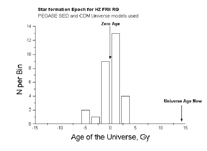
Figure 8: The age distribution of the star formation epoch for the PEGASE model in the CDM model of the Universe.

References

- [1] Arimoto N., Yoshii Y., 1987, Astron. Astrophys., 179, 23
- [2] Benn C.R., Wall J., Vigotti M., Grueff G., 1989, Mon. Not. R. Astron. Soc., 235, 465
- [3] Barabaro S., Olivi F.M., 1991, Astron. J., 101, 922
- [4] Chambers K., Charlot S., 1990, Astrophys. J. Lett., 348, L1
- [5] Cowie L., Hu E.M., Songaila A., 1995, Nature, 377, 603
- [6] Dunlop J., Peacock J., Spinrad H., Dey A., Jimenez R., Stern D., Windhorst R., 1996, Nature, 381, 581
- [7] Dodonov S.N., Parijskij Yu.N., Goss W.M., Kopylov A.I., Soboleva N.S., Temirova A.V., Verkhodanov O.V., Zhelenkova O.P., 1999, Astron. Zh., 76 (in press)
- [8] Fanaroff B.L., Riley J.M., 1974, Mon. Not. R. Astron. Soc., 167, 31P
- [9] Fioc M., Rocca-Volmerange B., 1997, Astron. Astrophys., 326, 950
- [10] Krauss L., 1997, Astrophys. J., 480, 466
- [11] Kurutz R., 1992, in: “The stellar population of Galaxies”, IAU Symp. No 149, ed. Barbuy B., Penzini A., Kluwer Dordrecht, 225
- [12] Lilly S., 1987, Mon. Not. R. Astron. Soc., 229, 573
- [13] Lilly S., 1990, in: “Evolution of the Universe”, ed. Kron R.G., Astron. Soc. Pacific, 344.
- [14] Lancon A., Rocca-Volmerange B., 1992, Astron. Astrophys. Suppl. Ser., 96, 593.
- [15] McCarthy P.J., 1993, Annu. Rev. Astron. Astrophys., 31, 639
- [16] Parijskij Yu. N., Goss W.M., Kopylov A.I., Soboleva N.S., Temirova A.V., Verkhodanov O.V., Zhelenkova O.P., Naugolnaya M.N., Bull. Spec. Astrophys. Obs., 40, 1996, 5
- [17] Parijskij Yu.N., Soboleva N.S., Temirova A.V., Kopylov A.I., Verkhodanov O.V., 1997, Prepr. SAO No. 121, St.Petersburg
- [18] Poggianti B.M., 1997, Astron. Astrophys., 122, 399
- [19] Rocca-Volmerange B., Guiderdoni B., 1988, Astron. Astrophys. Suppl. Ser., 75, 93
- [20] Schlegel D., Finkbeiner D., Davis M., 1998, Astrophys. J., 500, 525
- [21] von Hoerner S., 1974, in: “Galactic and extragalctic radio astronomy”, eds. G.L.Verschuur & K.I.Kellermann, Springer-Verlag
- [22] Verkhodanov O.V., 1996, Bull. Spec. Astrophys. Obs., 41, 149
- [23] Verkhodanov O.V., Kopylov A.I., Parijskij Yu.N., Soboleva N.S., Temirova A.V., 1998a, in: “Aktualnye problemy vnegalakticheskoi astronomii” (“Current Problems of Extragalactic Astronomy”), Proc. XV Conf., Pushchino, May 25–29, Pushchino Sci. Center, 24
- [24] Verkhodanov O.V., Kopylov A.I., Parijskij Yu.N., Soboleva N.S., Temirova A.V., Zhelenkova O.P., 1998b, in: “Prospects of Astronomy and Astrophysics For the New Millennium”. Joint European and National Astronomical Meeting, JENAM’98. 7th Europ. & 65th Ann. Czech Astron. Conf., Prague, 9-12 Sept., 302