Identification of a complete sample of northern ROSAT All-Sky Survey X-ray sources

Abstract

We present the statistical evaluation of a count rate and area limited complete sample of the ROSAT All-Sky Survey (RASS) comprising 674 sources. The RASS sources are located in six study areas outside the galactic plane ($|b^{II}|\ga 20^{\circ}$) and north of $\delta=-9^{\circ}$. The total sample contains 274 (40.7%) stars, 26 (3.9%) galaxies, 284 (42.1%) AGN, 78 (11.6%) clusters of galaxies and 12 (1.8%) unidentified sources. These percentages vary considerably between the individual study areas due to different mean hydrogen column densities $N_{\rm H}$. For the accuracy of the RASS positions, i.e., the distance between optical source and X-ray position, a 90% error circle of about 30″ has been found. Hardness and X-ray-to-optical flux ratios show in part systematic differences between the different object classes. However, since the corresponding parameter spaces overlap significantly for the different classes, an unambiguous identification on the basis of the X-ray data alone is not possible. The majority of the AGN in our sample are found at rather low redshifts with the median value of the whole sample being $z_{\rm med}=0.24$. The median values for the individual fields vary between $z_{\rm med}=0.15$ and $z_{\rm med}=0.36$. The slope of the $\log\,N\,-\,\log\,S$ distributions for our AGN ($-1.44\pm 0.09$) is in good agreement with the euclidian slope of $-1.5$. The BL Lacs (with a slope of $-0.72\pm 0.13$) exhibit a much flatter distribution.

1 Introduction

The ROSAT All-Sky Survey (RASS) was the first all-sky survey in the soft X-ray range (0.07 keV to 2.4 keV) with an imaging telescope (Aschenbach Aschenbach88 (1988)). It started on July 30, 1990, two months after the launch of the ROSAT X-ray satellite (Trümper Trumper83 (1983)) on June 1, 1990. Using the Position Sensitive Proportional Counter (PSPC) ROSAT scanned the sky during the All-Sky Survey in great circles perpendicular to the direction of the sun, and thus covered the whole sky in half a year. The RASS allowed for the first time to study unbiased, spatially complete samples of X-ray sources. Previous knowledge of the composition of the X-ray sky at high galactic latitudes was mainly based on the EINSTEIN Medium Sensitivity Survey (EMSS) (Stocke et al. Stockeetal91 (1991)) containing serendipitious sources found in X-ray images of fields with otherwise scientifically interesting objects.

On the basis of the X-ray data alone it is usually not possible to determine the physical nature of the X-ray source. In order to do so, optical follow-up observations have to be carried out. Since during the RASS about 60 000 sources were detected (Voges et al. Vogesetal99 (1999)), it is obvious that a complete identification of all sources is beyond any reasonable scope. In order to obtain representative subsamples six study areas from the RASS were selected for a complete optical identification. These study areas are located north of $\delta=-9^{\circ}$, with $|b^{II}|\ga 20^{\circ}$ including one region near the North Galactic pole (NGP) and one near the North Ecliptic Pole (NEP).

A detailed description of the fields, the selection criteria, the optical observations and the criteria for the optical identification bave been extensively discussed in Zickgraf et al. (Zickgrafetal97a (1997)), hereafter Paper II. As described in Paper II, in order to reduce the sample to a manageable but still statistically significant size, we chose minimum count rates of 0.03 cts s^-1 for five of our areas and 0.01 cts s^-1 for one area. A catalogue of the complete optical identifications of our flux limited sample is presented in Appenzeller et al. (Appenzelleretal98 (1998)), hereafter Paper III. On the basis of this paper we shall give in the following a detailed statistical analysis of the final results from our identification programme.

2 Basic Statistics

Some basic statistical information on the optical identifications in our six study areas is given in Table 1. The field designations are essentially those defined in Table 1 of Paper II. However, for study areas IV and V we have used a slightly modified field definitions: Study area IV of this paper corresponds to IVac of Paper II, and study area V to Va of Paper II. We note, that the designations used here correspond to those already used in Paper III.

The first row of Table 1 gives the number of sources in the individual study areas which fulfill our flux criteria mentioned above. In the second row the number of sources is given for which the identification exclusively rests on a comparison with the SIMBAD or NED data bases. The third row gives the number of sources observed by ourselves (91.8% of all sources).

Table 1: Basic statistical information on the identifications. The class “stars” includes normal stars, Ke, Me stars, CVs, binaries, and white dwarfs.

study area	I	II	III	IV	V	VI	total
No. of sources:	100	122	124	110	125	93	674
SIM/NED id.:	6	20	12	8	6	3	55
Observed:	94	102	112	102	119	90	619
Identified:	100	120	120	109	123	90	662
stars	63	52	43	13	43	34	248
galaxies	2	6	9	4	0	2	23
AGN	19	44	48	68	55	38	272
clusters of gal.	7	8	11	14	22	10	72
multiple sources	9	10	9	10	3	6	47
no id.	0	2	4	1	2	3	12

In the lower part of the table the number of identified sources for different object classes as well as the number of unidentified sources is given. Only for a total of 12 sources (1.8%) no identification could be found. This fraction is lower by more than a factor of two than the 3.9% unidentified sources in the EMSS (Stocke et al. Stockeetal91 (1991)). As already mentioned in Paper III, there are 21 sources (3.1%) for which we have a likely, but uncertain identification (’identification quality index’ Q=3 in Table 1 of Paper III). A discussion of these sources can be found in the comments on the individual sources in Paper III. In the following we shall not distinguish these cases from the reliable identifications.

For 47 X-ray sources (7.0%) (’mult. sources’ in Table 1) two possible optical counterparts were found (cf. the discussion in Paper II). In Paper III both sources are listed in the order of likelihood or suspected relative contribution to the total X-ray flux. Table 2 lists the number of ’pairs’ of object classes for these multiple sources:

Table 2: Distribution of multiple sources according to object classes

. star - star: 19 star - AGN: 11 star - gal: 1 star - galaxy cl: 6 AGN - AGN: 2 AGN - gal: 2 AGN - galaxy cl: 2 gal - galaxy cl: 4

Of the 47 multiple sources 37 (78%) contain at least one star. For our statistical purposes we consider as the optical identification the more likely source which is listed first in column 12 of Paper III. (The same procedure was applied by Stocke et al. Stockeetal91 (1991) for the EMSS.)

2.1 Distribution of sources

With the inclusion of the more plausible parts of the multiple sources we obtain the following distribution of all identified sources for the complete sample: stars: 274 (40.7%), galaxies: 26 (3.9%), AGN: 284 (42.1%) and clusters of galaxies: 78 (11.6%). Table 3 lists this distribution along with the distribution in the individual fields and a detailed subdivision of the object classes.

Table 3: Number distribution of optical counterparts for the different study areas. The abbreviations mean: ES: hot emission line star (including cataclysmic variables), S: Seyfert galaxy, Nl1: Narrow line Seyfert 1 galaxy, AGN uncl.: Active galactic nucleus for which a more accurate classification was not possible from our spectra, int. gal.” interacting galaxy.

study area	I	II	III	IV	V	VI	total
No. of sources:	100	122	124	110	125	93	674
Stars:	70	60	48	15	44	37	274
A stars:	2	0	1	0	0	0	3
F stars:	13	14	8	2	12	4	53
G stars:	15	16	8	3	2	10	54
K stars:	11	7	11	4	13	8	54
M stars:	0	1	1	1	1	1	5
Ke stars:	9	9	7	0	5	5	35
Me stars:	17	7	10	5	8	6	53
ES:	1	6	2	0	2	3	14
WD:	2	0	0	0	1	0	3
Act. gal. nuc.:	20	45	50	74	56	39	284
S1:	11	22	32	43	20	18	146
S1.5:	1	0	0	3	2	4	9
S2:	0	2	3	4	3	4	16
LINER:	0	2	0	1	0	0	3
NL1:	1	1	0	0	0	1	3
QSO:	3	8	9	18	24	8	70
BL Lac:	3	9	4	4	7	3	30
AGN uncl.:	1	1	2	1	1	1	7
Galaxies	3	6	11	4	0	2	26
normal:	2	2	10	2	0	1	17
int. gal.:	0	1	0	1	0	0	2
radio gal.:	1	3	1	1	0	1	7
Galaxy clusters:	7	9	11	16	23	12	78

Nearly the same fraction of stars and AGN are found in our RASS sample (40.7% and 42.1%, respectively). Together they represent nearly 83% of all sources. This differs significantly from the distribution of sources in the EMSS (Stocke et al. Stockeetal91 (1991)). The RASS sample shows a much higher fraction of stellar counterparts than the EMSS (40.7% vs. 25.8%), but a lower fraction of AGN (42.7% vs. 54.5%). The fraction of clusters of galaxies is with 11.6% (RASS) and 12.2% (EMSS) about the same in both samples. The same applies for galaxies with 3.9% (RASS) and 2.7% (EMSS) which do not show significant differences either.

More than half of all Active Galactic Nuclei were found to be Seyfert 1 galaxies. Alltogether the Seyfert galaxies form 62.3% of the AGN counterparts. About 25% are QSO and the fraction of BL Lac objects amounts to 10.6% This fraction corresponds to 4.5% of the whole sample which is nearly the same fraction as found for the EMSS. However, among the AGN the fraction of the BL Lac objects is with 7.8% somewhat lower in the EMSS.

2.2 Stellar counterparts

Among the stellar counterparts K stars (including Ke stars) occur most frequently (32.5%). F, G and M/Me stars have about the same frequency (19.3, 19.7, and 21.2%, respectively). About 39% of the K star and more than 90% of the M star counterparts display emission lines. This obviously reflects the fact that emission lines in the optical spectrum indicate strong stellar activity which tends to give rise to X-ray emission. The frequency of Ke stars may have been underestimated, since at our low spectral resolution weak emission lines could not always be detected.

In order to check whether some of our stellar identifications could be due to a random positional coincidence with field stars, we calculated the number of stars $n_{\rm err}$ expected for the total area of our 674 error circles (0.147 deg²). For our calculations we used the luminosity function by spectral type presented in Table 4-7 by Mihalas & Binney (MihalasBinney81 (1091)). For the scale heights in $z$ direction we used the numbers given in Table 4-16 by Mihalas and Binney. The numbers for $n_{\rm err}$ were calculated for Galactic Latitude $b^{\rm II}$ of 45 degrees. Interstellar extinction was not taken into account.

For both F and M stars random positional coincidences do not play any significant role. For F stars brighter than our detection limit of $V\sim$ 14 mag we expect 0.8 stars in the total area of our error circles, for M stars brighter than the limit of $V$ = 15 mag we expect 0.3 stars, respectively.

The situation is different, however, for G and K stars. Here we expect for stars down to a brightness limit of $V$ = 15 mag some 7.6 and 6.6 stars, respectively, in the total area of our error circles. For a brightness limit of 13 we expect for the G stars still 3.4 stars in the error circles, whereas for the K star the expectation value of 0.8 stars drops below one. The expectation value of one star per error circle area is reached for G stars at $V\sim$ 12 mag.

These results show that the number of dwarf stars randomly present in the total area of our error circles should be of the order of $\sim$15 sources. However, the actual number of G stars fainter than 12th magnitude and K stars fainter than 13th magnitude incorrectly identified as X-ray sources due to a random positional coincidence, should be much lower. Firstly, as all G and K stars emit X-rays at some level, it is unlikely that all the stars in the error circles are unrelated to the observed X-ray flux. Secondly, as most error circles contain another plausible optical counterpart (such as an AGN), the majority of the randomly present dwarf stars are expected to appear as the less probable component in multiple sources. (There are nine multiple sources, where we considered a faint G or K star to be the less likely counterpart). Thirdly, a source with, for instance, a bright AGN and a faint dwarf star normally has not been classified as multiple source. Therefore, even with most pessimistic assumptions a random positional coincidence should not have resulted in more than about two to three G and the same number of K stars incorrectly identified as optical counterparts of the observed X-ray sources. These numbers are significantly smaller than the $\sqrt{n}$ statistical uncertainties of our results for these stars and, therefore, do not affect our statistical conclusions.

Our resolution was, unfortunately, not sufficient, to detect the lithium $\lambda$6707 absorption line which would be an indicator for a relatively young age of the star. In a follow-up study of the present identification project, Zickgraf et al. Zickgrafetal98 (1998) found among 35 K and M stars of field I nine stars which display significant Li $\lambda$6707 absorption. First results of a detailed study of field VI by Zickgraf et al. (in preparation) indicate that here the fraction of Li stars among the K stars is lower than in field I.

We note that three A stars (two A2, one A5) were found in our sample. This is unexpected, since, according to theoretical predictions, early to mid A stars should not show any X-ray emission because of the missing convection zone (e.g. Haisch & Schmitt Haisch96 (1996)). In most cases, where X-ray emission seemed to be present in A stars, it was found to originate from a cool companion.

2.3 Comparison of individual fields

As can be seen from Table 3, there are in part distinct differences between the individual fields. While in field I the stellar counterparts outnumber the AGN by a factor of 3.5, there are 5 times more AGN than stars in field IV. These differences are of high statistical significance. The main reason for this differing ratios are different mean hydrogen column densities $N_{\rm H}$. In field I $<N_{\rm H}>(11.5\cdot 10^{20}$ cm${}^{-2})$ is more than seven times higher than in field IV (1.6$\cdot 10^{20}$ cm^-2). The main reason for this strongly differing hydrogen column density is the location at different galactic latitudes $b^{II}$. While field I is at an intermediate galactic latitude $b^{II}\sim-37^{\circ}$, field IV is close to the North Galactic Pole (mean latitude $b^{II}\sim+84^{\circ})$.

In fields II, III, V, and VI the ratios n_stars/n_AGN are between 0.79 (field V) and 1.33 (field II). In fields III and VI about the same numbers of stars and AGN have been identified. These four fields have - with $<N_{\rm H}>$ values between 3.9$\cdot 10^{20}$ and 5.5$\cdot 10^{20}$ cm^-2 - intermediate mean hydrogen column densities. For these fields no correlation between the ratio of stars and AGN with $<N_{\rm H}>$ could be found.

2.4 Accuracy of the RASS positions

With our complete sample it is possible to derive final values for the positional uncertainty of RASS X-ray sources, i.e., the mean distance of the identified optical sources from the X-ray positions. We follow the same procedure as outlined in section 5.2 of Paper II. Figure 1 shows the positional uncertainties in right ascension (solid line) and in declination (dashed line) of our sources. 1 $\sigma$, (i.e. the 67% error circle) corresponds to 13.5″ for right ascension and 12.8″ for declination, i.e. about the same for each coordinate. The sytematic offset towards the east due to the motion of the satellite during read-out of the data is 1.5″. The standard deviation found here is about 4″ larger than in the preliminary data presented in Paper II.

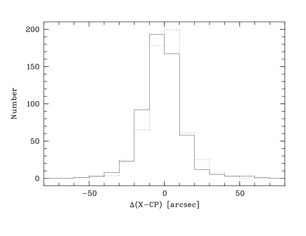
Figure 1: Histograms of the positional uncertainties. The differences in arcsec between X-ray position (’X’) and optical counterpart position (’CP’) are plotted separately for RA (solid line) and DEC (dashed line).

For the total distance between the optical source and the X-ray position we derive a 1 $\sigma$ standard deviation of 17″ and a 90% error circle of 30″. These numbers are significantly smaller than those calculated by the SASS (Standard Analysis Software System) where a 90% error circle of 40-45″ was derived (Voges et al., in preparation) and also smaller than the 50″ 90% confidence radii from the EMSS (Stocke et al. Stockeetal91 (1991)).

Because of the smaller area of the error circle of the RASS as compared to the EMSS, confusion of X-ray sources should be lower in the RASS than in the EMSS. Stocke et al. (Stockeetal91 (1991)) found for their EMSS a source confusion level of the order of 2.5% (21 out of 835 sources). Since the sensitivity levels of the RASS and the EMSS are not too different, we conclude that source confusion in our flux limited RASS sample should be well below 1%.

3 X-ray, optical and radio quantities

3.1 Hardness ratios

Tables 4 and 5 show mean hardness ratios of our samples. (For the definition of the hardness ratios see e.g. Paper II). For the calculation of the mean values only hardness ratios with internal errors $\sigma\leq 0.5$ have been used. In addition, all hardness ratios below -1.0 and above +1.0 were set to -1.0 and +1.0, respectively. Values of $|HR1|\geq 1.0$ are purely artificial without physical meaning. They arise from the fact that for very soft or and for very hard sources the X-ray flux in the hard or soft range, respectively, is below the detection limit. So fluctuations in the background subtraction can give (physically meaningless) negative values in these bands.

For the individual study areas mean hardness ratios have been calculated for stars and AGN only. For the three other groups, galaxies, cluster of galaxies, and sources with no optical identification (which are included for completeness reasons) the number of objects in the individual fields is too low to get any significant results.

As Tables 4 and 5 show, for the mean values of HR2, which subdivides the hard range, there are only marginal differences between the individual classes of objects. This applies to both the total sample and to the individual fields. Even in the case of strongly differing $<$HR1$>$ values are found (like for the AGN in fields I and IV, +0.83 vs. -0.12), the $<$HR2$>$ values are essentially the same. There is a trend that galaxies and clusters of galaxies seem to have somewhat higher $<$HR2$>$ values than stars.

For $<$HR1$>$ more pronounced differences are found between the individual classes of objects. Stars have on the average the lowest HR1, i.e., they have the softest spectral energy distributions (SED). This holds even, if one removes the white dwarfs and the emission line stars (cf. Paper III) from the sample, since $<$HR1$>$ changes from +0.11 to +0.12 only. AGN display on the average ($<$HR1$>$=+0.35) a somewhat harder SED than stars.

A significantly harder SED is found for clusters of galaxies with $<$HR1$>$=+0.65$\pm$0.26. This is indeed what is expected for this class of objects which exhibit a rather hard intrinsic spectrum caused by thermal bremsstrahlung from a hot (10⁷-10⁸ K) plasma (cf. e.g. Böhringer Boehringer96 (1996)).

For isolated galaxies $<$HR1$>$=+0.66$\pm$0.31 has been found. This is nearly the same mean hardness ratio as found for clusters of galaxies and that strongly supports the presumption discussed in Paper II that most of the isolated galaxies found in the RASS are in fact members of groups or even cluster of galaxies. The limited field of our optical images may not always have allowed to recognize the cluster. The X-ray data themselves provide little evidence, since the extension parameter given by the ROSAT SASS is, as discussed by Kneer (Kneer96 (1996)), of limited use only for the identification of clusters of galaxies.

Table 4: Mean hardness ratios HR1 and HR2. ’No. of sources’ gives the number of sources which fulfill the selection criteria discussed in the text.

study area
	I	II	III	IV	V	VI	total
stars
No. of sources	52	44	36	13	43	25	213
$<$HR1$>$	+0.01$\pm$0.49	+0.16$\pm$0.40	+0.08$\pm$0.37	-0.09$\pm$0.25	+0.14$\pm$0.37	+0.30$\pm$0.53	+0.11$\pm$0.43
$<$HR2$>$	+0.04$\pm$0.30	+0.10$\pm$0.34	+0.04$\pm$0.30	+0.15$\pm$0.39	-0.02$\pm$0.24	+0.01$\pm$0.32	+0.05$\pm$0.31
AGN
No. of sources	13	40	47	64	54	33	251
$<$HR1$>$	+0.83$\pm$0.17	+0.59$\pm$0.26	+0.39$\pm$0.33	-0.13$\pm$0.34	+0.43$\pm$0.34	+0.65$\pm$0.27	+0.35$\pm$0.43
$<$HR2$>$	+0.30$\pm$0.30	+0.22$\pm$0.27	+0.20$\pm$0.29	+0.12$\pm$0.29	+0.17$\pm$0.25	+0.19$\pm$0.30	+0.18$\pm$0.28

Taken both hardness ratios together, there is no galaxy and only one cluster with negative values in both bands. Since this conclusion is based on a total of 93 objects, one may safely conclude that two negative hardness ratios are very rare for galaxies and cluster of galaxies, even in fields with very low hydrogen column densities.

For the AGN pronounced variations of the $<$HR1$>$ values have been found between the individual fields. For field IV one gets a softer average X-ray spectrum of the AGN with $<$HR1$>_{IV}$=-0.13$\pm$0.34, whereas for field I one gets a very hard AGN spectrum with $<$HR1$>_{I}$=+0.83$\pm$0.17 with no HR1 below +0.39. For the whole sample individual HR1 values as low as -0.83 were found. These differences of the HR1 hardness ratios reflect mainly the differences in the absorbing hydrogen column densities. For the other four fields the mean ratios $<$HR1$>$ are between +0.39 and +0.65, i.e., in between the two extreme values. It is interesting that the second highest value of +0.63 is found in field VI which exhibits the second highest value of $N_{\rm H}$ too.

For the stars the situation is different. There are no significant differences in the mean HR1 ratios between the individual fields, not even between fields I and IV, for which significant differences have been found for the AGN. The fact that there are no differences in the mean hardness ratios between the stellar samples in fields which differ by about a factor of seven in the hydrogen column density wheras there are siginificant differences in the hardness ratios for the extragalactic sources clearly shows that at least the vast majority of all our stellar counterparts must be located in front of the absorbing hydrogen. We note that the mean $N_{\rm H}$ values are not based on our X-ray data, but, as discussed in Paper II, on radioastronomical measurements compiled by Dickey & Lockman (DickeyLockman90 (1990)).

With the exception of two sources there are no stellar sources in the area of hardness ratios with both HR1 $\geq$ 0.0 and HR2 $\geq$ +0.5, whereas the other three classes of objects fairly densely populate this area. With the exception of a few very soft sources there are no stellar objects with HR1 $\leq$ -0.45. However, the very soft sources are a somewhat special case, since they have the major fraction of their X-ray flux in the soft band and only little or nothing at all in the hard band. This means that usually HR2 is not well defined and affected by a large error. If one includes also sources with high errors in HR2 one obtains a total of 22 sources with HR1 $\leq$ -0.5. Including these sources in the total sample of stellar counterparts one obtains $<$HR1$>$=+0.03$\pm 0.47$ which is slightly lower than the value given in Table 4.

Table 5: Mean hardness ratios HR1 and HR2 for galaxies, clusters and X-ray sources without optical counterparts for the total sample.

	galaxies	clusters	no ident.
No. of sources:	25	72	9
$<$HR1$>$	+0.66$\pm$0.31	+0.65$\pm$0.26	+0.43$\pm$0.39
$<$HR2$>$	+0.27$\pm$0.39	+0.22$\pm$0.30	+0.26$\pm$0.39

3.2 X-ray-to-optical flux ratios

As already noted by earlier studies (e.g. Maccacaro et al. Maccacaroetal88 (1988) or Stocke et al. Stockeetal91 (1991)) the X-ray-to-optical flux ratios differ significantly between the object classes. Therefore, for the identification of their objects they used this criterion in order to pre-select the sources they actually observed. While this methods leads in many cases to reliable pre-identification, it is nevertheless obvious that this pre-selection does also bias any statistical derivation of the X-ray-to-optical flux ratio.

In the present study, as discussed in Section 4 of Paper II, a somewhat different approach had been chosen for the identification of the optical counterparts. There was no pre-selection according to the X-ray-to-optical flux ratio. Only in doubtful cases the X-ray-to-optical flux ratio was used (as well as hardness ratios HR1 and HR2) as secondary criterion for the identification. Hence, the X-ray-to-optical flux ratios of our sample should be less biased than those of the EMSS.

The conversion of count rates to fluxes which depends on the intrinsic spectral energy distribution and on the hydrogen column density has been extensively discussed in Paper II. Figs. 2 and 3 show X-ray-to-optical flux ratios log$[f_{x}$/$f_{V}]$ vs. the optical flux $f_{V}$ for various object classes. In Table 6 the limits of the log[$f_{x}$/$f_{V}$] ratios as well as average values are given. Clusters of galaxies are not included, since, contrary to the EMSS sample, in our case usually no brightness has been determined for the individual members of the clusters.

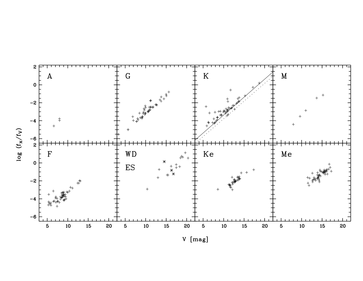
Figure 2: X-ray-to-optical flux ratios log$[f_{x}$/$f_{V}]$ vs. the optical flux $f_{V}$ for the stars in our sample. The letters denote the spectral type. ’WD’ means white dwarf (asterisks) and ’ES’ emission line star (crosses). The lines plotted in the diagram of the K stars are lower flux limit for coronal sources (see text).

The lower boundaries of the distributions shown in Figs. 2 and 3 are determined by the count limit chosen. As already mentioned, they depend on the spectral energy distribution assumed and the hydrogen column density. For demonstration purposes we have plotted in the diagram of the K stars the lower limit for coronal sources with the flux limit of 1.8$\cdot$10^-13 erg s^-1 cm^-2 (solid line) given in Table 3 of Paper II. In addition, we have also plotted the lower limit for 0.6$\cdot$10^-13 erg s^-1 cm^-2 for field V (dashed line) which has the lowest hydrogen column density. It is obvious that the sources below the lower boundaries are missed in our sample because of the count rate limit.

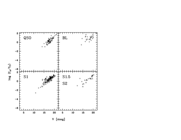
Figure 3: X-ray-to-optical flux ratios log$[f_{x}$/$f_{V}]$ vs. the optical flux $f_{V}$ for various classes of AGN.

Table 6: Ranges and average values of X-ray-to-optical flux ratios for various classes of objects.

Object class	log$[f_{x}$/$f_{V}]_{limits}$		$<log[f_{x}$/$f_{V}]>$
	min	max
starstot	-5.52	+1.13	-2.46$\pm$1.27
A stars	-4.59	-3.78	-4.11$\pm$0.42
F stars	-4.82	-1.97	-3.70$\pm$0.68
G stars	-5.52	-0.80	-2.89$\pm$1.02
K stars	-4.57	+0.20	-2.77$\pm$1.04
M stars	-4.41	-1.14	-2.68$\pm$1.37
Ke stars	-2.99	-0.76	-2.02$\pm$0.51
Me stars	-2.51	-0.14	-1.33$\pm$0.50
WD	-1.22	+0.14	-0.63$\pm$0.70
ES	-2.91	+1.13	-0.42$\pm$1.12
AGNtot	-2.62	+2.02	+0.41$\pm$0.65
S1	-2.62	+1.40	+0.37$\pm$0.61
S1.5	-1.01	+0.61	+0.07$\pm$0.61
S2	-1.22	+1.43	+0.47$\pm$0.86
QSO	-1.00	+1.71	+0.35$\pm$0.57
BL Lac	-0.56	+2.02	+0.94$\pm$0.54
Galaxies	-2.14	+1.61	-0.27$\pm$0.92

As compared with the EMSS, most object classes in the RASS sample display a somewhat wider range in the $<log[f_{x}$/$f_{V}]>$ ratios, even if one takes into account that in the numbers given in Stocke et al.’s Table 1 objects with extreme values are excluded. This means that in the RASS samples there are larger overlapping areas which do not allow an unequivocal pre-selection on the basis of the $<log[f_{x}$/$f_{V}]>$ ratios. This is shown in Fig. 4 which displays the ranges of $\log f_{\rm x}/f_{V}$ listed in Table 6.

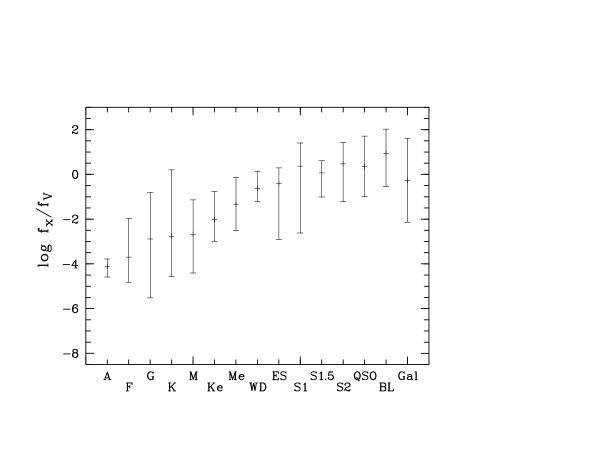
Figure 4: Mean values and ranges of $\log f_{\rm x}/f_{V}$ as listed in Table 6 for the different classes of X-ray emitters. The various classes overlap considerably.

In particular we would like to note that there is a large overlapping area between the stars and the AGN, even if one excludes white dwarfs and cataclysmic binaries which show the highest $<log[f_{x}$/$f_{V}]>$ ratios among the stellar counterparts.

The large difference for the maximal values for galaxies can be explained by the fact that a significant fraction of the galaxies in the RASS sample are, as discussed above, indeed groups or clusters of galaxies. Another striking difference is the presence of a significant number of AGN with $<log[f_{x}$/$f_{V}]>\>$ 1. In the EMSS only very few AGN with such high ratios of X-ray-to-optical flux have been found. A possible explanation for this difference could be that the limiting magnitudes of the optical identifications for the RASS sample are lower than those of the EMSS, since the highest X-ray-to-optical flux ratios are indeed found for the faintest objects.

As one would expect for the stellar counterparts in our sample (cf. e.g. Schmitt Schmitt90 (1990)), the maximal value of the $<log[f_{x}$/$f_{V}]>$ ratio increases with decreasing T_eff. On the average, Ke and Me stars show, as expected (see 2.2), higher X-ray luminosities than the K and M stars without emission lines. The Ke and Me stars display a much smaller range of $<log[f_{x}$/$f_{V}]>$ ratios than the normal K and M stars which is either due to the fact that no X-ray faint Ke and Me stars are found or simply, that there were no optically bright emission line stars in our sample.

3.3 Stellar counterparts

Fig. 5 shows the visual brightness distribution of the stellar counterparts. It peaks around around 11th to 13th magnitude which is due to the large number of K and M stars in this brightness range. Among the faintest counterparts ($V\ga 17$) objects classified ”ES” dominate, i.e. mostly cataclysmic variables (hashed histogram in Fig. 5).

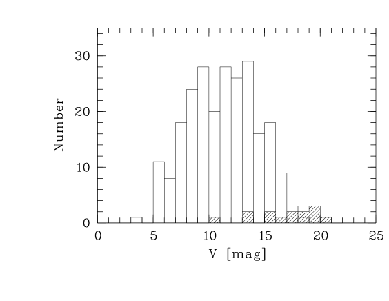
Figure 5: Histogram showing the number distribution of the visual brightness of the stellar counterparts. The class ”ES” is separately plotted as hashed histogram.

Fig. 6 shows the $\log\,N\,-\,\log\,S$ distribution for the stellar sample, excluding objects of classes “ES” and “WD”. For fluxes below $1.8\,10^{-13}$ erg s^-1 cm^-2 the smaller survey area of study area V has been taken into account (cf. Paper II). The slope in the range $S_{\rm x}=2\,10^{-13}-10^{-11}$ erg s^-1 cm^-2 is $-1.36\pm 0.11$ (maximum likelihood), hence slightly flatter than expected for the Euclidian slope of $-1.5$. This indicates that our sample is affected by the scale height of the galactic distribution of the stellar counterparts.

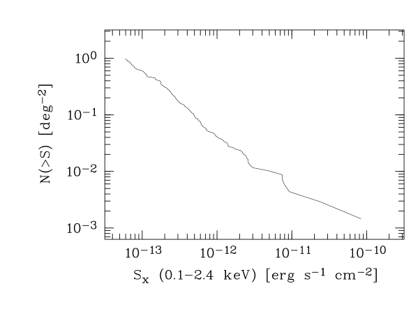
Figure 6: Area-corrected $\log\,N\,-\,\log\,S$ distribution for stellar counterparts (exluding classes “ES” and “WD”).

3.4 Active Galactic Nuclei

3.4.1 Redshift distribution

The redshift distribution of the AGN of the whole sample is presented in Fig. 7. As can be seen, the majority of the AGN in our sample are found at rather low redshifts with the median value of the whole sample being z_med=0.24. The median values for the individual fields vary between z_med=0.15 and z_med=0.36. The highest value of z_med=0.36 is found in field V where the minimum count rate of 0.01 cts s^-1 is lower by a factor of 3 as compared to 0.03 cts s^-1 in the other five fields. The second highest median z value z_med=0.31 is found in field IV which is the field with the lowest $N_{\rm H}$. Correspondingly, the lowest median value z_med=0.15 for the redshift distribution is found in field I, the field with the highest $N_{\rm H}$.

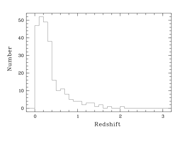
Figure 7: Redshift distribution of the AGN of the whole sample. Not included is the quasar at z=4.28

We note that the highest redshift z=4.28 found for the quasar RXJ1028.6-0844 (Zickgraf et al. Zickgrafetal97b (1997)) is one of the highest redshifts at all found for RASS sources.

3.4.2 $\log\,N\,-\,\log\,S$ distributions

Because of the limited RASS exposure time as well as the flux limit chosen by us (cf. Paper II), only the brighter AGN show up in our RASS sample. Hence, our sample is the ideal complement to the deep surveys where preferentially low-luminosity AGN are found. Both data sets combined allow to construct a $\log\,N\,-\,\log\,S$ function which covers a wide range of luminosities and which can be used for cosmological studies. This has been done and discussed by Lehmann et al. Lehmannetal98 (1998) and Miyaji et al. Miyajietal98 (1998) who combined our sample with 207 ksec PSPC observations of the Lockman Hole and with the 1.112 Msec HRI ultradeep survey observations (Hasinger et al. Hasingeretal98 (1998)).

In order to correct for the variation of the survey area as a function of flux, we computed $\log\,N\,-\,\log\,S$ distributions by taking the area as displayed in Fig. 8 into account. We used the flux limits given in Paper II for each of the individual study areas. The area drops from the total of 685 deg² at fluxes 10^-12 erg s^-1 cm^-2 in several steps at the individual limiting fluxes to 37 deg², which is the size of area V. The area corrected $\log\,N\,-\,\log\,S$ distributions for all AGN and for the BL Lac objects in our sample are diplayed in Fig. 9. The distributions are linearly increasing towards the lowest flux. For the AGN no indication of a flattening due to incompleteness is indicated except at the lowest fluxes.

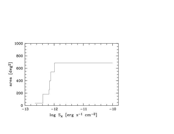
Figure 8: Survey area as a function of flux. The limiting fluxes for the individual study areas were taken from Paper II.

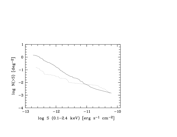
Figure 9: Area-corrected $\log\,N\,-\,\log\,S$ distributions for AGN (solid line) and BL Lacs (dashed line).

The slope of the $\log\,N\,-\,\log\,S$ distributions for AGN is with $-1.44\pm 0.09$ in good agreement with the euclidian slope of $-1.5$. The BL Lacs exhibit with a slope of $-0.72\pm 0.13$ a much flatter distribution. The errors have been calculated using the formula given by Crawford et al. (Crawfordetal70 (1970)) basing on the maximum-likelihood technique. We suspect that the much lower slope of the BL Lac objects is due to incompleteness. In addition, it could be that a major fraction of the 12 undidentified sources are in fact BL Lac objects. Moreover, due to the low number (30) of BL Lacs our $\log\,N\,-\,\log\,S$ distribution is affected by statistical uncertainties.

A rather flat $\log\,N\,-\,\log\,S$ distribution for BL Lacs has been also found by Bade et al. Badeetal98 (1998), who studied a sample of 37 BL Lac objects from the RASS. In their sample the $\log\,N\,-\,\log\,S$ curve starts to flatten at 8$\cdot$10^-12 erg cm^-2 s^-1 which, taking into account their different energy range (0.5-2.0 keV) this corresponds to 1.8 $\cdot$10^-12 erg cm^-2 s^-1 in our energy range (0.07-2.4 keV). However, contrary to the above conclusions for our sample they do not ascribe this flattening to incompleteness. For our RASS sample the $\log\,N\,-\,\log\,S$ curve for BL Lacs lies slightly above the curve found by Bade et al. Unfortunately, it is not possible to compare the redshift and luminosity distributions of the two samples, since the low resolution spectra used for our optical identification did not allow us to derive the redshifts of the BL Lac objects.

3.4.3 Radio fluxes

The radio fluxes at 4.85 GHz, the X-ray flux $f_{\rm x}$ in the 0.1-2.4 keV energy range, and the $B$ magnitudes given in Paper III were used to calculate the continuum slopes $\alpha_{\rm ro}$ and $\alpha_{\rm ox}$. The definition of these coefficients is given e.g. in Stocke et al. (Stockeetal91 (1991)). The optical fluxes at 2500 Å were derived from the the $B$ magnitudes using the relation given by Schmidt (Schmidt68 (1968)) for $\alpha_{\rm o}=-0.5$. For BL Lacs we assumed $\alpha_{\rm o}=-1.4$ (Ghisellini et al. Ghisellinietal86 (1986)). The monochromatic X-ray flux at 2 keV was obtained from the integrated flux $f_{\rm x}$ using a photon index of -2. Radio fluxes at 4.85 GHz from the 87GB catalog listed in Paper III were K-corrected for spectral index $\alpha_{\rm r}=-0.5$ for QSOs and Seyfert galaxies, 0.0 for BL Lacs, and -0.7 for galaxies. For BL Lacs a redshift of 0.3 was assumed for those without measured $z$. The resulting $\alpha_{\rm ro}$-$\alpha_{\rm ox}$ diagram is shown in Fig. 10.

The sources are distributed in a similar way as shown in Stocke et al. (Stockeetal91 (1991)) (cf. their Fig. 6) with the exception that our sample contains only a few radio-quiet objects (with respect to the limits shown in Stocke et al.). This is due to the flux limit of the 87GB catalog. Most of the BL Lacs are located in a region between $\alpha_{\rm ro}=0.3$ and 0.5 which is separated from that occupied by the radio-loud QSOs and Seyferts, although some overlap exists in particular at large $\alpha_{\rm ox}$. The extension of the BL Lac region towards larger $\alpha_{\rm ox}$ also contains three radio galaxies. At least for the X-ray bright BL Lacs (i.e. small $\alpha_{\rm ox}$) a reliable classification based on the $\alpha_{\rm ox}$ - $\alpha_{\rm ro}$ diagram is possible. Likewise, both radio-loud and X-ray-bright AGN are well separated in the upper left corner of the diagram.

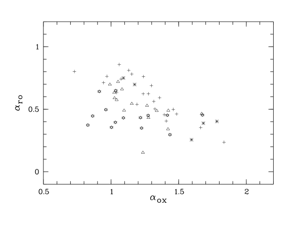
Figure 10: $\alpha_{\rm ro}$-$\alpha_{\rm ox}$ diagram for QSOs ($+$), Seyfert galaxies (triangles), BL Lacs (star symbols), and radio galaxies (asterisks).

4 Conclusions

The results of a complete optical identification of a spatially complete, count rate limited of ROSAT All-sky survey X-ray sources show that the RASS is dominated by stellar sources and AGN. While nearly the same fraction of stars and AGN (40.7% and 42.1%, respectively) are found in our total sample which comprises six individual fields outside the galactic plane, distinct variations are found between the individual fields. The main parameter responsible for these variations is the mean hydrogen column density $N_{\rm H}$ in the field which, however affects more the number of AGN than the stars. As the distribution of the mean hardness ratios $<$HR1$>$ shows, at least the vast majority of the stellar sources must be located in front of the absorbing hydrogen.

For the accuracy of the RASS positions, i.e., the total distance between optical source and X-ray position, a 90% error circle of about 30″ has been found. This error circle is considerably lower than the 40-45″ found by the SASS which is basing on X-ray data alone.

Hardness and X-ray-to-optical flux ratios vary between the different object classes. However, since there are in the corresponding parameter spaces large overlapping areas between the different classes, an unambiguous identification on the basis of the X-ray data alone is not possible. Optical follow-up observations are therefore indispensable for an identification.

RASS data are the ideal complement to deep surveys for e.g. constructing $\log\,N\,-\,\log\,S$ distributions for cosmological studies. In the RASS mainly objects at the bright end of the X-ray luminosity function are found. However, because of its large spatial area a significant number of the high luminosity objects which have a low space density are found.

Because of the low resolution used for the spectroscopy in this identification project more detailed investigations, such as searches for Li $\lambda$6707 absorption in stellar sources were not possible. However, as first publications based on our catalog show, the results of our identification program offers a rich mine for many more detailed follow-up studies.

- (1) Appenzeller, I., Thiering, I., Zickgraf, F.-J., et al., 1998, ApJS 117, 319 (Paper III)
- (2) Aschenbach, B., 1988, Appl. Optics, 27, 1404
- (3) Bade, N., Beckmann, V., Douglas, N.C., Barthel, P.D., Engels, D., Cordis, L., Nass, P., Voges, W., 1998, A&A 334, 459
- (4) Böhringer, H., 1996. In: H.U. Zimmermann, J.E. Trümper, H. Yorke (eds.), MPE Rreport 263, “Röntgenstrahlung from the Universe”, Garching 1996, p. 537
- (5) Crawford, D.F., Jauncey, D.L., Murdoch, H.S., 1970, ApJ 162, 405
- (6) Dickey J.M., Lockman F.J., 1990, ARA&A 28, 215
- (7) Ghisellini G., Maraschi L., Tanzi E.G., Treves A., 1986, ApJ 310, 317
- (8) Haisch, B., Schmitt, J.H.M.M., 1996, PASP 108, 113
- (9) Hasinger G.R., Burg R., Giacconi R., et al., 1998, A&A 329, 482
- (10) Kneer R., 1996, Ph.D. thesis, University of Heidelberg
- (11) Lehmann, I., Hasinger, G., Schwope, A., Boller, T., 1998, in: Proceedings of the Symposium “Highlights in X-ray Astronomy in honour of Joachim Trümper’s 65th birthday”, eds. B. Aschenbach & M.J. Freyberg, MPE Report 269 (in press)
- (12) Maccacaro, T., Gioia, I., Wolter, A., Zamorani, G., Stocke, J., 1988, ApJ 326, 680
- (13) Mihalas, D., Binney, J., Galactic Astronomy, 1981, W. H. Freeman and Company, San Francisco
- (14) Miyaji, T., Hasinger, G., Schmidt, M., 1998, in: Proceedings of the Symposium “Highlights in X-ray Astronomy in honour of Joachim Trümper’s 65th birthday”, eds. B. Aschenbach & M.J. Freyberg, MPE Report 269 (in press)
- (15) Schmidt, M., 1968, ApJ 151, 393
- (16) Schmitt, J.H.M.M., 1990, Adv. Space Res. 10, 115
- (17) Stocke, J.T., Morris, S.L., Gioia, I.M., et al., 1991, ApJS 76, 813
- (18) Trümper, J., 1983, Adv. Space Res. vol. 2, No. 4, 241
- (19) Voges W., Aschenbach B., Boller, Th., et al., 1999 A&A 349, 389
- (20) Zickgraf, F.-J., Thiering, I., Krautter, J., et al., 1997, A&AS 123, 103 (Paper II)
- (21) Zickgraf, F.-J., Voges, W., Krautter, J., Thiering, I., Appenzeller, I., Mujica, R., Serrano, A., 1997, A&A 323, L21
- (22) Zickgraf, F.-J., AlcalaÁ, J.M., Krautter, J., Appenzeller, I., Sterzik, M.F., Motch, C., Pakull, M.W. 1998, A&A 339, 457