Hubble Space Telescope weak lensing study of the $z=0.83$ cluster MS 1054-03¹

Abstract

We have measured the weak gravitational lensing of faint, distant background galaxies by MS 1054-03, a rich and X-ray luminous cluster of galaxies at a redshift of $z=0.83$, using a two-colour mosaic of deep WFPC2 images. The small corrections for the size of the PSF and the high number density of background galaxies obtained in these observations result in an accurate and well calibrated measurement of the lensing induced distortion.

The strength of the lensing signal depends on the redshift distribution of the background galaxies. We used photometric redshift distributions from the Northern and Southern Hubble Deep Fields to relate the lensing signal to the mass. The predicted variations of the signal as a function of apparent source magnitude and colour agrees well with the observed lensing signal. The uncertainty in the redshift distribution results in a 10% systematic uncertainty in the mass measurement.

We determine a mass of $(1.2\pm 0.2)\times 10^{15}~{}h_{50}^{-1}~{}{\rm M}_{\odot}$ within an aperture of radius 1 $h_{50}^{-1}$ Mpc. Under the assumption of an isothermal mass distribution, the corresponding velocity dispersion is $1311^{+83}_{-89}$. For the mass-to-light ratio we find $269\pm 37h_{50}{\rm M}_{\odot}/{\rm L}_{B\odot}$ after correcting for pass-band and luminosity evolution. The errors in the mass and mass-to-light ratio include the contribution from the random intrinsic ellipticities of the source galaxies, but not the (systematic) error due to the uncertainty in the redshift distribution. However, the estimates for the mass and mass-to-light ratio of MS 1054-03 agree well with other estimators, suggesting that the mass calibration works well.

The reconstruction of the projected mass surface density shows a complex mass distribution, consistent with the light distribution. The results indicate that MS 1054-03 is a young system. The timescale for relaxation is estimated to be at least 1 Gyr.

We have also studied the masses of the cluster galaxies, by averaging the tangential shear around the cluster galaxies. Using the Faber-Jackson scaling relation, we find the velocity dispersion of an $L_{*}$ galaxy (${\rm L}_{B}=8\times 10^{10}h_{50}^{-2}{\rm L}_{B\odot}$ for MS 1054-03) is $203\pm 33$ km/s.

^⋆ Kapteyn Astronomical Institute, University of Groningen,
P.O. Box 800, 9700 AV Groningen, The Netherlands
e-mail: hoekstra, kuijken@astro.rug.nl
  
^† Leiden Observatory,
P.O. Box 9513, 2300 RA Leiden, The Netherlands
e-mail: franx@strw.strw.leidenuniv.nl

Accepted for publication in the ApJ

Subject headings: cosmology: observations $-$ gravitational lensing $-$ dark matter $-$ galaxies: clusters: individual (MS1054-03)

1 Introduction

Studying the mass distribution of massive clusters at high redshifts is important as their existence puts strong constraints on possible cosmological models (e.g. Eke et al. 1996; Bahcall & Fan 1998; Donahue et al. 1998). Furthermore, these systems may be young and thus much can be learned about the formation of massive clusters of galaxies.

Massive structures in the universe induce a systematic distortion of the images of faint background sources, providing a powerful diagnostic to study their mass distributions (e.g. Mellier 1999). The weak lensing signal allows us to map the projected mass surface density of the lens (e.g. Kaiser & Squires 1993), and determine its mass. Although the weak lensing mass estimate does not require assumptions about the dynamical state or geometry, it does require a good estimate for the redshift distribution of the faint sources.

Since Tyson, Wenk, & Valdes (1990) succesfully measured the systematic distortion of faint galaxies by a foreground cluster, many massive clusters of galaxies have been studied (e.g. Bonnet, Mellier, & Fort 1994; Fahlman et al. 1994; Squires et al. 1996). These studies concentrated on massive clusters with redshifts $z\sim 0.2-0.5$.

Smail et al. (1994) tried to measure the weak lensing signal for the optically selected, high redshift cluster Cl 1603+43 $(z=0.89)$. Its observed velocity dispersion is $1226^{+245}_{-154}$ km/s (Postman, Lubin, & Oke 1998). Smail et al. (1994) used source galaxies down to a limiting magnitude of $I=25$, but failed to detect a signal. Their results are consistent with a lower mass for the cluster. This is supported by the cluster’s X-ray luminosity of $L_{x}(0.1-2.4~{}{\rm keV})=1.1\times 10^{44}h_{50}^{-2}$ ergs/s (Castander et al. 1994), which is an order of magnitude lower than the X-ray luminosity of the brightest, high redshift, X-ray selected clusters

The X-ray emission of clusters of galaxies provides an efficient means to select massive clusters of galaxies. Since the work of Smail et al. (1994), several high redshift, X-ray luminous clusters have been discovered from Einstein (Gioia & Luppino 1994) and ROSAT observations (Henry et al. 1997; Ebeling et al. 1999; Rosati et al. 1998).

Luppino & Kaiser (1997; LK97 hereafter) successfully detected the weak lensing signal from the X-ray selected, high redshift cluster MS 1054-03 using deep ground based imaging. Clowe et al. (1998) reported on the detection of weak lensing signals for the X-ray selected, high redshift clusters MS 1137+66 and RXJ1717+67, from deep Keck imaging. However, these studies suffered from the lack of knowledge of the redshift distribution of the faint sources.

Lensing studies of high redshift clusters are difficult because the lensing signal is low and most of the signal comes from small, faint galaxies. This is the regime where HST observations have great advantage over ground based imaging, because the background galaxies are much better resolved. As a result, higher number densities of sources can be reached, the images are not crowded, and more importantly the correction for the circularization by the PSF is much smaller. Especially for high redshift clusters, where the redshift of the lens approaches that of the sources, the lensing signal depends strongly on the redshift distribution of the sources.

In this paper we present our weak lensing analysis of the cluster MS 1054-03 using a mosaic of deep WFPC2 images. It is the second cluster we studied using a mosaic of deep HST observations. In Hoekstra et al. (1998, HFKS98 hereafter) we presented the analysis of Cl 1358+62, a rich cluster of galaxies at a redshift of $z=0.33$.

MS 1054-03 $(z=0.83)$ is the most distant cluster in the Einstein Extended Medium Sensitivity Survey (Gioia et al. 1990; Gioia & Luppino 1994). It is extremely rich and has a restframe X-ray luminosity $L_{x}(2-10~{}{\rm keV})=2.2\times 10^{45}h_{50}^{-2}$ ergs/s (Donahue et al. 1998), which makes it one of the brightest X-ray clusters known. From their ASCA observations Donahue et al (1998) find a high X-ray temperature of $12.3^{+3.1}_{-2.2}$ keV.

Our space based observations allow us to study the cluster mass distribution in much more detail than LK97. Photometric redshift distributions inferred from the Hubble Deep Field North (Fernández-Soto, Lanzetta, & Yahil 1999) and South (Chen et al. 1998) give a good approximation of the redshift distribution of the sources used in this weak lensing analysis. As a result it is possible to obtain well calibrated mass estimates for high redshift clusters of galaxies from multi-colour imaging, even if the availability of spectroscopic redshift data for the sources is limited.

The observations and data reduction are outlined in section 2. In section 3 we briefly discuss the method we use to analyse the galaxies. Section 4 deals with the light distribution of the cluster. In section 5 we present the measurements of the lensing induced distortions of the faint galaxies and the reconstruction of the projected mass surface density. Section 6 deals with the redshift distribution of the faint galaxies. Our mass determination is presented in section 7. In this section we also discuss several effects that complicate accurate mass determinations. The results for the mass-to-light ratio are given in section 8. In section 9 we examine in more detail the substructure of the cluster. The lensing signal due to the cluster galaxies themselves is studied in section 10.

2 Observations

In this analysis we use WFPC2 images taken with the Hubble Space Telescope (GO proposal 7372, PI Franx). Figure 2 shows the layout of the mosaic constructed from the 6 pointings of the telescope. The integration time per pointing was 6400s in both the $F606W$ and $F814W$ filter. For the weak lensing analysis we omitted the data of the Planetary Camera because of the brighter isophotal limit. The total area covered by the observations is approximately 26 arcmin².

Fig. 1.—: Layout of the observed field. The six pointings are indicated and numbered. The positions of the 20 brightest cluster galaxies are indicated by the black dots. The dashed circle indicates an aperture with a radius of 1 $h_{50}^{-1}$ Mpc. The image is oriented such that North is up. The area covered by the observations is approximately 26 arcmin^-2.

For each pointing the exposures of a given passband were split into two sets. The images in each set were offset from each other by integer pixels ($\pm 3$ pixels). Both sets were reduced and combined separately, resulting in two images (for details see van Dokkum et al. 1999; van Dokkum 1999). These two images were designed to be offset by 5.5 pixels, to allow the construction of an interlaced image (e.g. Fruchter & Hook 1998; van Dokkum 1999), which has a sampling that is a factor $\sqrt{2}$ better than the original WFPC2 images.

Except for the images in the first pointing in F814W, all offsets were within 0.1 pixel of the requested value. We found that we had to omit the shape measurements in the $F814W$ band for pointing 1, because of the deviating offset for this exposure. However, we could use the $F606W$ image, and as the noise in the shear estimate is dominated by the intrinsic ellipticities of the galaxies, the loss in signal-to-noise is minimal.

3 Object analysis

Our analysis technique is based on that developed by Kaiser, Squires, & Broadhurst (1995; KSB95 hereafter) and LK97, with a number of modifications which are described in HFKS98.

The first step in the analysis is the detection of the galaxy images, for which we used the hierarchical peak finding algorithm from KSB95. We selected objects with a significance $\nu$ larger than $5\sigma$ over the local sky. The detected objects were analysed, yielding estimates for the sizes, magnitudes and shapes of the objects. The detection and analysis were done per WFPC2 chip and filter. As a new feature, our software computes an estimate for the error on the polarization from the data. This error estimate is discussed in Appendix A.

The resulting catalogs were inspected visually in order to remove spurious detections, like diffraction spikes, HII regions in resolved galaxies, etc. 4402 objects were detected in the $F606W$ images, whereas the $F814W$ images yielded 4290 stars and galaxies. The combined catalog consisted of 5848 stars and galaxies, of which 2844 were detected in both filters.

Fig. 2.—: Plot of the apparent magnitude in the F606W filter (upper panel) and the F814W filter (lower panel) versus half light radius. In both figures the vertical locus where stars are found is easily identified.

For all detected objects we estimated the apparent magnitude using an aperture with a diameter of $6\sqrt{2}r_{g}$ pixels (where $r_{g}$ is the Gaussian scalelength of the object as given by the peak finding algorithm). We converted the measured counts to $F606W$ and $F814W$ magnitudes, zero-pointed to Vega, using the zeropoints given in the HST Data Handbook (STScI, Baltimore). We added 0.05 magnitude to the zero-points to account for the Charge Transfer Efficiency (CTE) effect.

Figure 3 shows the apparent magnitude versus the half light radius of the object. Moderately bright stars are easily identified as they are located in the vertical locus. Bright stars saturate and hence their measured sizes increase. Using figure 3 we selected a sample of moderately bright stars, which were used to examine the PSF.

To obtain a catalog of galaxies we removed the stars from the catalog. At faint levels the discrimination between stars and galaxies is not possible, but by extrapolating the number counts of moderately bright stars to faint magnitudes, we find that the stars contribute less than 2% to the total counts.

We attempted to determine colours for all detected objects (including galaxies detected in only one filter), using the same aperture in both filters. The software failed to determine colours for some of the galaxies. Most of these were extremely faint, and detected only in the $F814W$ band. For the weak lensing analysis we only used galaxies for which colours were determined. Due to this selection we lost 30% of the galaxies fainter than $F814W=26.5$ (533 galaxies).

The shape parameters of the galaxies were corrected for the PSF (cf. section 3.1) and the camera distortion We used the estimated errors on the shape measurements (cf. Appendix A) to combine the results from the $F606W$ and $F814W$ images in an optimal way, resulting in a final catalog of 4971 galaxies.

The better sampling of the interlaced images improved the object detection and analysis significantly. HFKS98 showed that due to the poor sampling of WFPC2 images only the shapes of galaxies with sizes $r_{g}>0\hbox{$.\!\!^{\prime\prime}$}12$ could be measured reliably. The images used here allow us to use all detected galaxies. HFKS98 found a number density of 79 galaxies arcmin^-2 from 3600s exposures in both $F606W$ and $F814W$. The observations presented here yield a number density of 191 galaxies arcmin^-2. This higher number density is due to both the longer integration time, and the improved sampling of the interlaced images. An analysis of the effect of small pointing errors in the interlaced images shows that these are not important for our analysis (cf. Appendix B).

Figure 3.1 shows the observed number counts of galaxies in our observations versus apparent magnitude. For comparison we also show the counts from the HDF-North (Williams et al. 1996). This indicates that our catalog of galaxies is complete down to $F606W=26.5$ and $F814W=26$.

3.1 Corrections

Several observational effects systematically distort the images of the galaxies. To obtain an accurate and unbiased estimate of the weak lensing signal these effects have to be corrected for. To do so, we follow the scheme outlined in KSB95, LK97, and HFKS98.

Fig. 3.—: Plot of the number counts of detected galaxies in the $F606W$ band (solid circles) and $F814W$ band (open triangles). The dashed line shows the number counts from the HDF-N (Williams et al. 1996) in the $F814W$ filter, and the solid line shows the counts in the $F606W$ filter. This indicates that our catalog is complete down to $F606W=26.5$ and $F814W=26$.

Fig. 4.—: The polarization field of stars taken from the interlaced observations in the F814W filter. The orientation of the sticks indicates the direction of the major axis of the PSF, whereas the length is proportional to the size of the anisotropy. The polarization values are measured using a Gaussian weight function with a dispersion of $0\hbox{$.\!\!^{\prime\prime}$}07$. The lower left panel corresponds to chip 2, lower right to chip 3, and the upper right one denotes chip 4. We have omitted chip 1, which is the planetary camera.

HFKS98 showed that the PSF of WFPC2 is highly anisotropic at the edges of the chips. We selected a sample of moderately bright stars from the observations of MS 1054. Figure 3.1 shows the observed polarization of these stars in the F814W band. The anisotropy pattern is similar to the pattern presented in HFKS98.

Because the PSF changes slightly with time, we fitted the shape parameters of our new observations to a scaled model of the PSF polarization measured from the globular cluster M4 and added a first order polynomial:

$$p_{i}^{\rm new}=a\cdot p_{i}^{\rm old}+c_{0}+c_{1}x+c_{2}y.$$

This procedure gave excellent fits to the observed PSF anisotropy in our observations of MS 1054.

The PSF also circularizes the images of the small, faint galaxies, thus lowering the amplitude of the lensing signal. Compared to ground based observations, the small faint galaxies are much better resolved in HST observations, resulting in much smaller corrections for the circularization by the PSF. This allows us to measure a well calibrated lensing signal.

To obtain estimates for the real shapes of the faint galaxies, we determined the ’pre-seeing’ shear polarizability $P^{\gamma}$ (LK97; HFKS98). The measurements of $P^{\gamma}$ for individual galaxies are rather noisy, and therefore we binned the data as a function of size of the object.

Fig. 5.—: Required correction factor $1/P^{\gamma}$ to estimate the ’pre-seeing’ ellipticity of the object. The solid line shows the results for the $F606W$ filter, and the dashed line shows the correction factor for $F814W$. The pre-seeing shear polarizability $P^{\gamma}$ corrects for the circularization by the weight function and the PSF. It depends strongly on the size of the object, and increases rapidly as the object’s size approaches the size of the PSF. As the PSF in ground based data is much larger, the corrections for galaxies of similar sizes would be much larger. The upper panel shows the cumulative number of objects as a function of size. The objects for which the peak finder assigned a size smaller than the PSF are analysed with a fixed weight function matched to the PSF. These objects end up in the bin of the smallest objects.

Fig. 6.—: Colour-magnitude diagram of the objects for which colours could be determined. The cluster colour-magnitude relation is clearly visible. The errorbars at the bottom of the plot correspond to the errorbars on the $F814W$ magnitude.

The results are presented in figure 3.1, which shows the required correction factor to obtain the true ellipticity of a galaxy from the observed polarization. The upper panel shows the cumulative number of objects as a function of object size. The objects for which the peak finder assigned a size smaller than the PSF were analysed with a weight function matched to the PSF. These objects end up in the bin corresponding to the smallest objects.

The correction for objects with sizes comparable to the size of the PSF is large. The PSF in ground based images is much larger, and therefore large correction factors are required for objects that are still well resolved in HST images. From a $0\hbox{$.\!\!^{\prime\prime}$}65$ deep ground based image we found that $P^{\gamma}\approx 0.2$ for galaxies of $R\sim 25$, whereas galaxies of similar brightness in our HST images have $P^{\gamma}\approx 0.6$.

As a test of our procedure we compared the distortion measured from the $F606W$ images and the $F814W$ images (which included the correction for the circularization) using only objects for which shape parameters could be measured in both images. We compared the average tangential distortions and found that the results for the two filters agree well to one another (we found $\langle g_{T}\rangle=0.0366\pm 0.0066$ from the $F606W$ data and $\langle g_{T}\rangle=0.0375\pm 0.0068$ for the $F814W$ images).

Recently it has been found that the Charge Transfer Efficiency problem for WFPC2 has worsened. This can systematically change the shapes of the faint galaxies, as charge is ’smeared’ along the CCD columns. This could result in a detectable change in the shapes of the galaxy images.

We compared the shapes of the objects in the regions where the pointings overlap (cf. figure 2). Unfortunately the number of objects was low, and the contribution of shot noise to the shape estimates substantial. We did not detect a systematic change in the shapes, but we cannot put strong constraints on the size of the effect. We also simulated the effect, assuming that the change in shape increased linearly with row number for each chip, with no change at low row numbers and a shear of 10% at high row numbers. We found that this resulted in a neglegible change in our mass estimate.

4 Light distribution

Figure 6 shows a plot of the colour of the galaxies versus their $F814W$ magnitude. The cluster is visible as the concentration of galaxies with $F606W-F814W\sim 2$. The galaxies on this colour-magnitude relation are generally early type galaxies, which are among the reddest objects in the cluster.

We selected 324 galaxies brighter than $F814W=24.5$, lying close to the colour-magnitude relation, to study the cluster light distribution. This catalog was compared to the spectroscopic catalog (van Dokkum 1999). The contamination by field galaxies is small, and we removed galaxies with redshifts incompatible to that of the cluster. Many of these belong to a small group at $z=0.547$ (van Dokkum 1999).

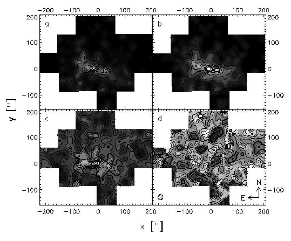
Fig. 7.—: (a) Luminosity distribution of cluster galaxies brighter than $F814W$ 24.5. The contours are 10%, 20%, etc. of the peak value; (b) Number density distribution of this sample of cluster galaxies; (c) Number density distribution of all detected galaxies brighter than $F814W$ 25; (d) Number density distribution of all detected galaxies fainter than $F814W$ 25, where we corrected the counts for the area covered by the (large) bright galaxies. In panels b–d the interval between subsequent contours are 20 galaxies arcmin^-2, and the thick lines indicate levels of 100 and 200 galaxies arcmin^-2. All distributions have been smoothed with a Gaussian filter with a FWHM of 20 arcseconds (indicated by the shaded circle). The mosaic covers approximately 26 arcmin^-2, and the total field shown is 7 by 6 arcmin.

We have use SExtractor (Bertin & Arnouts 1996) to determine total magnitudes for these galaxies. Figure 7 shows grey scale plots of the luminosity and number density weighted light distributions. The images have been smoothed with a Gaussian with a FWHM of 20 arcseconds. The galaxy number density and the luminosity weighted distributions look quite similar. The cluster light distribution is elongated east-west, and three clumps can be identified.

Figure 7 also shows gray scale images of the smoothed number density when we split the sample of all detected galaxies into a bright ($F814W<25$) and a faint sample ($F814W>25$). The cluster is clearly visible in the bright sample, but does not show up in the number counts of the faint galaxies (which have been corrected for the area covered by large bright galaxies). Figure 7d shows several significant peaks, indicative of some clustering at high redshift.

We estimate the luminosity in the redshifted $B$ band following van Dokkum (1999). The direct transformation from the HST filters to the passband corrected $B$ band is given by

$$B_{z}=F814W-0.03(F606W-F814W)+1.23,$$

where $B_{z}$ denotes the passband corrected $B$ band magnitude. The luminosity is given by

$$L_{B}=10^{0.4(M_{B\odot}-B_{z}+DM+A_{F814W})}L_{B\odot},$$

where $M_{B\odot}=5.48$ is the solar absolute $B$ magnitude, $DM$ is the distance modulus, and $A_{F814W}$ is the extinction correction in the $F814W$ filter towards MS 1054-03. The redshift of $0.83$ for MS 1054 gives a distance modulus of $44.09-5\log h_{50}$. Taking galactic extinctions from Burstein & Heiles (1982) we use a value of 0.03 for $A_{F814W}$.

At faint magnitudes, the colour-magnitude relation is less clearly defined. To estimate the total light of the cluster, an estimate of the amount of light contributed by galaxies fainter than $F814W=24.5$ is required. To do so, we fitted a luminosity function to the sample of bright, colour selected cluster galaxies. We found that a Schechter function with $\alpha=-1.0$ and ${\rm M}_{B}^{*}=-21.8+5\log h_{50}$ $({\rm L}_{*}=8\times 10^{10}h_{50}^{-2}{\rm L}_{B\odot})$ could fit the observed counts of the sample of bright, colour selected cluster galaxies. For nearby clusters one typically finds ${\rm M}_{B}^{*}=-21.0+5\log h_{50}$ (eg. Binggeli, Sandage, & Tammann 1988), indicating that the galaxies in MS 1054-03 are approximately twice as bright as nearby cluster galaxies. This is in good agreement with the results of van Dokkum et al. (1998) who studied the fundamental plane in MS 1054-03. The luminosity function indicates that we miss approximately 5% of the light when not including the faint galaxies.

MS 1054-03 is a high redshift cluster and one might expect a relatively high fraction of blue cluster galaxies, which are too blue to be included in our colour selected sample of cluster galaxies. Comparison of our sample to a sample of bright, spectroscopically confirmed members (van Dokkum 1999) indicates that we miss 16% of the total light in the $B$ band.

The cumulative light profile as a function of radius from the centre for the sample of bright galaxies is presented in figure 5. The profile is multiplied by a factor $1.05\times 1.16$ to account for the light from the faint cluster galaxies and the bluest galaxies. The solid line corresponds to the observed profile, whereas the dashed line shows a isothermal profile for comparison. We estimate the total luminosity within an aperture of 1 $h_{50}^{-1}$ Mpc to be $1.0\times 10^{13}h_{50}^{-2}L_{B\odot}$.

5 Weak lensing signal

Due to the intrinsic ellipticities of the galaxies, their individual shape estimates are very noisy measurements of the lensing induced distortion. We therefore need to average the measurements of a large number of galaxies to obtain a useful estimate for the distortion $g$.

To estimate the average distortion, we weight each object with the inverse square of the uncertainty in the distortion, which includes the contribution of the intrinsic ellipticies of the galaxies and the shot noise in the shape measurement (cf. Appendix A):

Fig. 8.—: The cumulative, passband corrected, $B$ band luminosity as a function of radius from the assumed cluster centre. The solid line corresponds to the observed profile. The profile was calculated using the colour selected sample of cluster galaxies, and was corrected for the contribution of very blue galaxies and faint galaxies. The dashed line corresponds to an isothermal profile, which is shown for comparison. The arrow indicates a radius of 1 $h_{50}^{-1}$ Mpc.

$$\langle g_{i}\rangle=\frac{\sum g_{i,n}\sigma_{g,n}^{-2}}{\sum\sigma_{g,n}^{-2}}.$$ (1)

Selecting galaxies with $22<F814W<26.5$ and $F606W-F814W<1.6$ (the ’source’ sample from table 1), and smoothing using a Gaussian with a FWHM of 20 arcsec, we obtain the distortion field presented in figure 5. The sticks indicate the direction of the distortion, and the length is proportional to the amplitude of the distortion. It shows that on average the faint galaxies tend to align tangentially to the (elongated) cluster mass distribution, as expected from gravitational lensing.

The average tangential distortion $g_{T}$ in radial bins is a useful measure of the lensing signal. It is defined as $g_{T}=-(g_{1}\cos 2\phi+g_{2}\sin 2\phi)$, where $\phi$ is the azimuthal angle with respect to the assumed centre of the mass distribution. We assume that the position of the Brightest Cluster Galaxy defines the centre of the cluster. At large radii from the cluster centre, where we do not have data on complete circles, we account for possbile azimuthal variation of $g_{T}$ by fitting

$$g_{T}(r,\phi)=\langle g_{T}\rangle(r)(1+g_{2,c}\cos(2\phi)+g_{2,s}\sin(2\phi))$$ (2)

to the observed distortions. This procedure gives the correct value for an ellipsoidal mass distribution. Although the cluster appears elongated, no large azimuthal variations in the tangential distortion were found.

Fig. 9.—: Distortion field $g$ obtained from the sample of source galaxies, smoothing the data using a Gaussian with a FWHM of 20 arcsec (indicated by the shaded circle). The orientation of the sticks indicates the direction of the distortion, whereas the length is proportional to the amplitude of the signal. Due to gravitational lensing the images of the faint sources tend to align tangentially to the cluster mass distribution.

Fig. 10.—: (a) Tangential distortion as a function of radius from the cluster centre using the sample of source galaxies as defined in table 1. A clear lensing signal is detected, although the dependence of the signal on radius indicates a complex mass distribution. (b) Measured signal when the phase of the distortion is increased by $\pi/2$. If the signal observed in (a) is due to gravitational lensing, $g_{X}$ should vanish as is observed. In both figures the arrows indicate a radius of $1~{}h_{50}^{-1}$ Mpc.

The average tangential distortion as a function of radius is presented in figure 10a. In the absence of lensing, the points should scatter around zero. The figure shows a systematic tangential alignment of the sources. The dependence of the signal on radius is quite complicated, indicative of a complex mass distribution. The results of the two-dimensional mass reconstruction (cf. section 5.1) show that the sharp decrease in the tangential distortion around 40” is due to substructure in the cluster mass distribution.

As a test, figure 10b shows the results when the phase of the distortion is increased by $\pi/2$ (i.e. rotating the sources by $\pi/4$). In this case the signal should vanish if it is due gravitational lensing, as is observed.

We divide our sample of galaxies in several subsamples, based on their apparent magnitude and colours. Table 1 lists some details of the subsamples. It shows that even our ’bright’ sample in fact consists of rather faint galaxies.

(1)	(2)	(3)	(4)	(5)	(6)
name	$F814W$	$F606W-F814W$	# galaxies	$\bar{n}$	$\bar{m}$
	[mag]	[mag]		arcmin-2	[mag]
source	$22-26.5$	$<1.6$	2643	102	25.2
bright	$22-25$	$<1.6$	1137	44	24.2
faint	$25-26.5$	$-$	1906	73	25.8
blue	$22-26.5$	$<0.8$	1198	46	25.4
red	$22-26.5$	$0.8-1.6$	1445	55	25.1

Table 1:: Properties of the various subsamples taken from the final catalog of galaxies.

The tangential distortion profiles of the various subsamples are presented in figure 5. A clear lensing signal is detected for all subsamples. The signals of the bright and the faint sample are independent measurements, and agree well with one-another. Although the profiles of the blue and the red sample agree well, the difference in the amplitude of the lensing signal is clear. This is due to the fact that, on average, the redder galaxies are at lower redshifts than the blue galaxies. In section 6 the issue of the redshift distribution of the background galaxies is discussed in detail.

Fig. 11.—: Tangential distortion as a function of radius from the cluster centre for the various subsamples: (a) bright galaxies; (b) faint galaxies; (c) blue galaxies; (d) red galaxies. The signals for the bright and the faint galaxies are quite similar in both strength and shape. Although the shapes of the signals for the blue and the red sample are similar, the difference in strength of the signal is clear. In these figures the arrows indicates a radius of $1~{}h_{50}^{-1}$ Mpc.

5.1 Projected mass distribution

Figure 6 shows the reconstructed mass surface density based on the distortion field presented in figure 5. We used the maximum probability extension of the original KS algorithm (Kaiser & Squires 1993; Squires & Kaiser 1996), which does not suffer from some of the biases of the original KS93 inversion, and can be applied directly to fields with complicated boundaries. Several effects complicate a direct interpretation of the mass map (cf. section 7.1). However, if the distortions are relatively small, it gives a fair description of the cluster mass distribution.

The mass reconstruction shows that the cluster mass distribution is quite complex: three distinct peaks are visible. The positions of the peaks coincide fairly well with the peaks in the light distribution (cf. Fig. 7). The results presented in LK97 lacked the resolution to detect the substructure.

Donahue et al. (1998) studied the X-ray properties of MS 1054 and found that the distribution of the gas is elongated similar to the weak lensing mass distribution. They also find evidence for substructure. However, the peak in their map of the X-ray brightness coincides with the western clump. Deeper X-ray observations by Neumann et al. (1999) show that the peak in the X-ray is close to the central clump. In section 9 we investigate the substructure in more detail.

Towards the edges of the observed field the noise in the reconstruction increases rapidly, and therefore the significance of the structures at the edge of the field is low.

The reconstruction after increasing the phase of the distortion by $\pi/2$ is shown in figure 6b. As this corresponds to the imaginary part of the mass surface density, no signal should be present if the observed distortion is due to gravitational lensing. We find no significant large scale structures in this map.

6 Redshift distribution

To relate the observed lensing signal to a measurement of the mass one has to estimate the mean critical surface density

$$\Sigma_{\rm crit}=c^{2}(4\pi GD_{l}\beta)^{-1},$$

where $D_{l}$ is the angular diameter distance to the lens and

$$\beta=\left\langle{\rm max}\left(0,D_{ls}/D_{s}\right)\right\rangle,$$

where $D_{s}$ and $D_{ls}$ are the angular diameter distances from observer to the source and lens to the source respectively. The angular diameter distance to MS 1054-03 is 1.96 $h_{50}^{-1}$ Gpc, which yields $\Sigma_{\rm crit}=845\beta^{-1}h_{50}\hbox{${\rm M}_{\odot}{\rm pc}^{-2}$}$ (using $\Omega_{m}=0.3$, and $\Omega_{\Lambda}=0$).

The question that remains is the value of $\langle\beta\rangle$. The uncertainty in the redshift distribution of the sources has hampered the mass estimates from previous lensing studies of high redshift clusters of galaxies (LK97; Clowe et al. 1998).

Down to $I\sim 23$ the redshift distribution of galaxies is fairly well known from redshift surveys, but the galaxies used in weak lensing analyses are generally too faint to be included in spectroscopic surveys. However, photometric redshift distributions derived from broad band photometry of the Northern HDF (Fernández-Soto, Lanzetta, & Yahil 1999) and Southern HDF (Chen et al. 1998) may be used to obtain an estimate of $\langle\beta\rangle$ as a function of apparent magnitude and colour. The photometric redshift distributions can be compared to our data, because we use the same filters, and the catalogs are complete down to the magnitude limit of our weak lensing analysis $(F814W<26.5)$. Figure 7.1.2 shows the comparison of the weak lensing signal with the predicted trends based on the HDFs in independent magnitude and colour bins.

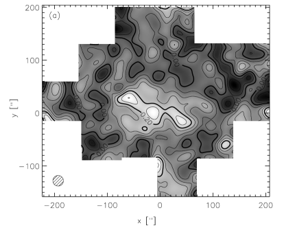
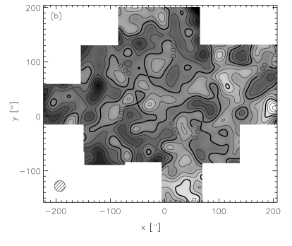
Fig. 12.—: (a) Reconstruction of the projected mass surface density. Towards the edges of the observations the signal-to-noise in the reconstruction decreases rapidly. The origin coincides with the assumed cluster centre. The reconstruction shows that the mass distribution consists of three distinct mass concentrations, similar to the light distribution. (b) The reconstructed mass surface density when the phase of the distortion is increased by $\pi/2$. As this projects out the imaginary part of the surface density, the signal should vanish if it is due to gravitational lensing. The mass distribution was smoothed using a Gaussian with a FWHM of 20” (indicated by the shaded circle). The interval between adjacent contours is 0.05 in $\kappa$.

Though there is some variation between the redshift distributions in the Northern and Southern fields, the results from the weak lensing analysis agree well with the predictions, giving us confidence that the calibration of the lensing signal using photometric redshifts works.

The average photometric redshift of $F814W<26.5$ galaxies in the HDF South is higher than it is in the Northern field. If this difference is representative of field to field variations the redshift distribution the uncertainty in weak lensing mass estimates of high redshift clusters $(z\sim 0.8)$ is significant: on the order of 10% (a bootstrapping analysis of the photometric redshift catalog indicates that the relative uncertainty in $\langle\beta\rangle$ for each individual deep field is only 2%). For clusters at lower redshifts the introduced uncertainty is smaller.

The value of $\langle\beta\rangle$ does not only depend on the redshifts of the sources, but it also depends on the cosmological parameters that define the angular diameter distances. Figure 7.1.2 shows how the average value of $\beta$ depends on $\Omega_{m}$ and $\Omega_{\Lambda}$ for MS 1054. For a given value of the cosmological constant, the dependence on $\Omega_{m}$ is weak, but given $\Omega_{m}$, the average value for $\beta$ is more sensitive to the value of the cosmological constant. In an $\Omega_{\Lambda}$ dominated universe the value of $\beta$ is approximately 20% higher than in a low $\Omega_{\Lambda}$ universe, and as a result the estimated mass for MS 1054-03 would be 20% lower.

In our estimates of the lensing signal we weight the contribution of each source according to its error on the distortion (cf. appendix A). Thus faint galaxies, which tend to be at higher redshifts are given less weight. Applying the same weight function (as a function of apparent magnitude) to the HDF galaxies shows that the effective average $\beta$ is slightly (6%) lower than the value indicated in figure 7.1.2. We use $\langle\beta\rangle=0.23$ $(\Omega_{\Lambda}=0)$ for our catalog of sources. Using $\Omega_{m}=0.3$ and $\Omega_{\Lambda}=0.7$ yields a higher value of 0.27 for $\langle\beta\rangle$.

7 Mass estimates

One of the advantages of gravitational lensing over other methods to estimate masses of clusters is that no assumptions have to made about the dynamical state or geometry. From the weak lensing signal we can directly estimate the projected mass within some aperture, although this requires rather good estimates for the redshift distribution of the background sources (cf. section 6).

However, several effects complicate a precise measurement of the total mass of a cluster. These are discussed in section 7.1. In section 7.2 we present our mass estimate for MS 1054-03. The result is compared to other estimators in section 7.3.

7.1 Complications in accurate mass determinations

7.1.1 Mass sheet degeneracy

The mass sheet degeneracy (Gorenstein, Shapiro, & Falco 1988) reflects the fact that the observed distortion is invariant under the transformation:

$$\kappa^{\prime}=(1-\lambda)\kappa+\lambda.~{}$$ (3)

Thus scaling the surface density, while adding a sheet of constant surface density, leaves the (observed) distortion unchanged. Measuring the distortion out to large radii, and arguing that the cluster surface density is neglegible at large radii, solves the problem if no intervening sheet of matter is present. In the analysis presented here we assume that this is the case.

The degeneracy can be lifted by measuring the magnification of the sources relative to an unlensed population of sources (e.g. Broadhurst, Taylor, & Peacock 1995). However, it is difficult to measure the magnification effect with sufficient accuracy to detect a mass sheet $\lambda$ of a few percent.

7.1.2 Measuring large distortions

Simulations of sheared images show that the correction scheme we use to measure the shapes of the galaxies works well for relatively small distortions $(\leq 0.3)$. The KSB95 approach assumes that the distortion is small everywhere. The pre-seeing shear polarizability $P^{\gamma}$ is derived from the average over all objects, and hence it is not accurate in the regime where

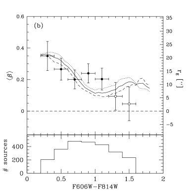
Fig. 13.—: (a) Comparison of the photometric redshift distribution with the observed weak lensing signal. The solid line is the predicted value of $\langle\beta\rangle$ as a function of apparent magnitude in the $F814W$ band, using the photometric redshift distribution of galaxies with $F606W-F814W<1.6$ and $F814W<26.5$. The dashed line shows the results using only the photometric redshifts from the HDF-North, and the dotted line gives the results for the Southern field. The variation in the value of $\langle\beta\rangle$ obtained from the two deep fields introduces an additional uncertainty in the weak lensing mass estimate. The points correspond to the weak lensing signal, which is obtained by a SIS model fit to the data ($\kappa(r)=r_{E}/2r$, where $r_{E}$ corresponds to the Einstein radius.) to the data at radii larger than 75 arcseconds. The right $y-$axis indicates the vertical scale in $r_{E}$. (b) The comparison as a function of colour of the background galaxies. We used galaxies with $22<F814W<26.5$. For the reddest bins (open circles), the contamination by cluster members is significant $(30-50\%)$, resulting in an underestimate of the lensing signal. The points in both figures are independent, and clearly show that the red galaxies carry a lower lensing signal and thus their average redshift is lower than that of the blue galaxies. The dependence of the lensing signal on the apparent magnitude is quite weak for the faint galaxies. In both figures the lower panels show a histogram of the number of objects in each bin. The widths of the bins are indicated by the horizontal errorbars.

Fig. 14.—: Contour plot of $\langle\beta\rangle$ as a function of $\Omega_{m}$ and $\Omega_{\Lambda}=1$, based on the photometric redshift distributions inferred from the HDF-N (Fernández-Soto et al. 1999) and HDF-S (Chen et al. 1998). For a given value of $\Omega_{\Lambda}$, the value of $\langle\beta\rangle$ depends only slightly on $\Omega_{m}$.

the distortions are large. When the average distortion is 0.4, the method already underestimates the distortion by 10%, and the discrepancy increases with increasing distortion. Other methods, like that proposed by Kuijken (1999), are more accurate when the distortion is large.

Due to the high redshift of MS 1054-03 the distortions are relatively small (cf. figure 10), and the KSB95 still works. However, placing the cluster at $z=0.2-0.4$ would produce much larger distortions, and the effect mentioned here has to be corrected for.

7.1.3 Converting $g$ to $\gamma$

The data provide a measure of the distortion $g$, which is related to the shear by $\gamma=(1-\kappa)g$. In the inner regions of the cluster, where $\kappa$ is significant, the factor $(1-\kappa)$ is important.

7.1.4 Broad redshift distribution

Another effect is related to the redshift distribution of the sources. When computing the average distortion, we use an average value for $\beta$ for the sources, i.e. we assume that the redshift distribution can be approximated by a sheet of sources at redshift corresponding to the average $\beta$. As we show now, this results in an overestimate of the lensing signal.

For an individual galaxy the distortion is

$$g=\frac{\gamma}{1-\kappa}=\frac{\beta_{s}\gamma_{\infty}}{1-\beta_{s}\kappa_{\infty}},$$ (4)

where $\kappa_{\infty}$ and $\gamma_{\infty}$ correspond to the dimensionless surface density and shear for a source at infinite redshift, and $\beta_{s}=\beta/\beta_{\infty}$. If we adopt a common value of $\beta$ for all background galaxies, we estimate the distortion as

$$\langle\tilde{g}\rangle=\frac{\langle\beta_{s}\rangle\gamma_{\infty}}{1-\langle\beta_{s}\rangle\kappa_{\infty}},$$ (5)

whereas the true average distortion is in fact given by the average of equation 4:

$$\langle\hat{g}\rangle=\left\langle{\frac{\beta_{s}\gamma_{\infty}}{1-\beta_{s}\kappa_{\infty}}}\right\rangle.$$ (6)

The ratio $\hat{g}/\tilde{g}$ indicates by what factor the shear $\gamma$ is overestimated. To first order it can be approximated by:

$$\frac{\langle\hat{g}\rangle}{\langle\tilde{g}\rangle}\approx 1+\left(\frac{\langle\beta_{s}^{2}\rangle}{\langle\beta_{s}\rangle^{2}}-1\right)\kappa=1+\left(\frac{\langle\beta^{2}\rangle}{\langle\beta\rangle^{2}}-1\right)\kappa.$$ (7)

This result was also derived by Seitz & Schneider (1997) in their analysis of non-linear mass reconstructions. Using the photometric redshift distributions for the HDFs, we find that for MS 1054-03, one would overestimate the shear by a factor $(1+0.62\kappa)$: this represents a 7% effect at a radius of 500 $h_{50}^{-1}$ kpc. The size of the effect increases with lens redshift as is demonstrated in figure 7.1.4.

Fig. 15.—: (a) Plot of $(\langle\beta^{2}\rangle/\langle\beta\rangle^{2}-1)$ as a function of lens redshift, based on the distribution of photometric redshifts from the HDF-N and HDF-S. To produce this figure we used galaxies with $F606W-F814W<1.6$ and $F814W<26.5$. The effect increases with lens redshift. (b) Plot of $(\langle\beta^{2}\rangle/\langle\beta\rangle^{2}-1)\kappa$ as a function of lens redshift. We used the value of $\kappa$ at a distance of 0.5$h_{50}^{-1}$ Mpc for a cluster with an isothermal mass distribution and a velocity dispersion of 1000 km/s. For MS 1054-03 the shear at this distance from the cluster centre would be overestimated by 7%.

7.1.5 Magnification

A further source of error arises from the fact that lensed images of background sources are not only distorted, but also magnified. Their total flux is increased by a factor $\mu=((1-\kappa)^{2}-\gamma^{2})^{-1}$. As a result the average redshift of the sources increases. The change in $\beta$ is approximately $2.2\kappa{\rm d}\beta/{\rm d}m$, which is small.

All mass estimates presented below have been corrected for the effects listed above. Since they are proportional to $\kappa$, they mainly affect the inner regions of the cluster.

7.2 Mass of MS 1054-03

To obtain an estimate of the mass of MS 1054, we fit a simple mass model to the data. It is straightforward to include corrections for the effects mentioned in section 7.1.1 into the model. However, the result depends on the assumed radial surface density profile, and given the complex mass distribution of MS 1054, fitting a simple model might not yield the best mass estimate. Nevertheless, it should give a fair indication of the mass (within a factor of 1.5, depending on the radial profile). We fitted a singular isothermal sphere model $(\kappa=r_{E}/2r)$ to the tangential distortion at radii larger than 75”. We found a value of $r_{E}=11\hbox{$.\!\!^{\prime\prime}$}5\pm 1\hbox{$.\!\!^{\prime\prime}$}4$, which corresponds to a velocity dispersion $\sigma=1365\pm 84$ km/s.

Another approach is often referred to as aperture mass densitometry. The shear can be related directly to a density contrast. We will use the statistic of Clowe et al. (1998), which is related to the $\zeta$ statistic of Fahlman et al. (1994):

$$\zeta_{c}(r_{1})=2\int\limits_{r_{1}}^{r_{2}}d\ln r\langle\gamma_{T}\rangle+2(1-\frac{r_{2}^{2}}{r_{\rm max}^{2}})^{-1}\int\limits_{r_{2}}^{r_{\rm max}}d\ln r\langle\gamma_{T}\rangle.$$ (8)

$\zeta_{c}$ yields the mean dimensionless surface density interior to $r_{1}$ relative to the mean surface density in the annulus from $r_{2}$ to $r_{\rm max}$:

$$\zeta_{c}(r_{1})=\bar{\kappa}(r^{\prime}<r_{1})-\bar{\kappa}(r_{2}<r^{\prime}<r_{\rm max}).$$ (9)

It shows that one can measure the average surface density within $r_{1}$ up to a constant if the shear were observable. We used the two-dimensional mass reconstruction, to obtain an estimate of the shear from the observed distortion.

Fig. 16.—: Plot of the $\zeta_{c}$ statistic as a function of radius from the assumed cluster centre. The values for $\zeta_{c}$ were calculated using the sample of source galaxies (cf. table 1), and using $r_{2}=105.2^{\prime\prime}$ (1 $h_{50}^{-1}$ Mpc) and $r_{\rm max}=200^{\prime\prime}$. At small radii it is difficult to correct for the effects mentioned in 7.1.1, and as a result these points are overestimates of the true values. The arrow indicates a radius of 1 $h_{50}^{-1}$ Mpc.

(1)	(2)	(3)	(4)	(5)	(6)	(7)
$\Omega_{m}$	$\Omega_{\Lambda}$	1 $h_{50}^{-1}$ Mpc	$\langle\beta\rangle$	$\Sigma_{\rm crit}$	$M(<1h_{50}^{-1}{\rm Mpc})$	$\sigma$
		[”]		$[\beta^{-1}h_{50}\hbox{${\rm M}_{\odot}{\rm pc}^{-2}$}]$	$[10^{15}h_{50}^{-1}{\rm M}_{\odot}]$	[km/s]
0.3	0.0	105.2	0.23	845	$1.25\pm 0.17$	$1311^{+83}_{-89}$
0.3	0.7	93.8	0.27	754	$1.07\pm 0.12$	$1215^{+63}_{-67}$
1.0	0.0	120.6	0.23	969	$1.38\pm 0.19$	$1379^{+89}_{-97}$

Table 2:: Mass estimates for various choices of $\Omega_{m}$ (1) and $\Omega_{\Lambda}$ (2); (3) angular scale of 1 $h_{50}^{-1}$ Mpc in arcseconds; (4) average $\beta$ for our catalog; (5) critical surface density; (6) mass within an aperture of 1 $h_{50}^{-1}$ Mpc radius; (7) corresponding velocity dispersion if the mass distribution were isothermal.

Figure 7.2 presents the measurement of $\zeta_{c}(r)$ using the sample of source galaxies as defined in table 1 (cf. Fig. 10), and taking $r_{\rm max}=200^{\prime\prime}$. At large radii from the cluster centre we cannot average the data on complete circles, and therefore we used equation 2 to estimate the average tangential shear. The results show that the surface density in the centre is quite high, making it difficult to accurately correct the measurements at small radii for the effects listed in section 7.1.1.

We find $\zeta_{c}=0.070\pm 0.014$ at a radius of 1 $h_{50}^{-1}$ Mpc (indicated by the arrow). This yields a lower limit on the mass within this aperture of $(8.0\pm 1.7)\times 10^{14}~{}h_{50}^{-1}~{}{\rm M}_{\odot}$. To obtain the total mass, we need to estimate the average surface density in the outer annulus. To this end we use the results of the SIS model fit. This gives $0.038\pm 0.005$ for the average dimensionless surface density in the outer annulus. Thus we find that the total mass within an aperture of 1 $h_{50}^{-1}$ Mpc is $(1.2\pm 0.2)\times 10^{15}~{}h_{50}^{-1}~{}{\rm M}_{\odot}$. If the mass distribution were isothermal, this mass estimate would correspond to a velocity dispersion of $1311^{+83}_{-89}$ km/s.

Table 2 lists the mass estimates for different cosmologies. It shows that the mass estimate for MS 1054-03 decreases for an increasing value of the cosmological constant.

The uncertainties in the mass estimates presented in this section only reflect the contribution from the intrinsic ellipticities of the source galaxies. As shown in section 6, the uncertainty in the redshift distribution of the sources may contribute an additional 10% systematic uncertainty.

7.3 Comparison with other estimates

For some time MS 1054-03 was the only very massive, X-ray selected, high redshift cluster known, and therefore it has been studied extensively.

LK97 were the first to detect a weak lensing signal for this cluster. The tangential distortion presented in LK97 is about a factor 1.5 higher than the signal from our HST observations (using galaxies with $21.5<F814W<25.5$). The difference in the signals might be due to the large corrections for the circularization by the PSF in the ground based observations of LK97. Furthermore, their mass estimate was hampered by the lack of knowledge of the redshift distribution of the faint galaxies.

Donahue et al. (1998) measured a high X-ray temperature of $12.3^{+3.1}_{-2.2}$ keV from ASCA observations, which corresponds to a velocity dispersion of $1400\pm 170$ km/s (90% confidence limits) under the assumption of an isothermal mass distribution. This estimate is in excellent agreement with our weak lensing mass estimate. However, the agreement is somewhat surprising: the cluster is clearly not relaxed, and one might expect that the gas is shock heated as the three massive clumps are merging.

The dynamical velocity dispersion was measured by van Dokkum (1999), who finds a value of $1150\pm 90$ km/s based on 81 galaxies. Earlier reported measurements based on smaller samples (Donahue et al. 1998; Tran et al. 1999) are consistent with this result.

All the evidence gathered so far indicates that MS 1054 is a very massive cluster, and using a Press-Schechter analysis one can estimate the likelihood of finding such a cluster in the EMSS catalog. Based on such analyses, LK97, and Donahue et al. (1998) have argued that the presence of MS 1054 in the EMSS catalog is hard to reconcile with $\Omega_{m}=1$. However, in an open or $\Omega_{\Lambda}$ dominated universe, the likelihood of finding massive high redshift clusters is much greater (e.g. Bahcall & Fan 1998). If the primordial density fluctuations are non-gaussian, the presence of MS 1054-03 in the EMSS catalog does not necessarily exclude a high density universe (Willick 1999).

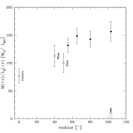
Fig. 17.—: Average mass-to-light ratio within an aperture for radii larger than 50 arcseconds from the cluster centre (filled circles). The mass in the aperture was estimated using equation 8 and assuming that the average dimensionless surface density in the outer annulus $\kappa(105{\hbox{$.\!\!^{\prime\prime}$}}2<r<200^{\prime\prime})=0.038\pm 0.005$. The points are correlated and the errorbars only reflect the uncertainty in the measurement of the distortion. The open circles denote the observed mass-to-light ratios of the three clumps in the mass distribution, using the results listed in table 4. The arrow indicates a radius of 1 $h_{50}^{-1}$ Mpc.

(1)	(2)	(3)	(4)	(5)
$\Omega_{m}$	$\Omega_{\Lambda}$	$L_{B}$	$M/L_{B}$	$M/L_{B}~{}(z=0)$
		$[10^{13}~{}h_{50}^{-2}L_{B\odot}]$	$[h_{50}{\rm M}_{\odot}/{\rm L}_{B\odot}]$	$[h_{50}{\rm M}_{\odot}/{\rm L}_{B\odot}]$
0.3	0.0	1.0	$124\pm 17$	$269\pm 37$
0.3	0.7	1.2	$90\pm 10$	$225\pm 25$
1.0	0.0	0.85	$163\pm 22$	$299\pm 41$

Table 3:: Average mass-to-light ratio within an aperture with a 1 $h_{50}^{-1}$ Mpc radius for different choices of the cosmological parameters (columns (1) and (2)); (3) Total light within the aperture; (4) observed average mass-to-light ratio in the passband corrected $B$ band; (5) mass-to-light ratio in the $B$ band, corrected for luminosity evolution as inferred from the evolution of the fundamental plane for the various choices of $\Omega_{m}$ and $\Omega_{\Lambda}$ (van Dokkum et al. 1998).

(1)	(2)	(3)	(4)	(5)	(6)	(7)
Clump	$\sigma_{SIS}$	$\zeta_{c}(26^{\prime\prime})$	$\bar{\kappa}(100^{\prime\prime}<r<150^{\prime\prime})$	M ($<250~{}h_{50}^{-1}$ kpc)	$L_{B}$	$M/L_{B}$
	[km/s]			$[10^{14}h_{50}^{-1}{\rm M}_{\odot}]$	$[10^{13}h_{50}^{-2}L_{B\odot}]$	$[h_{50}{\rm M}_{\odot}/{\rm L}_{B\odot}]$
East	$702\pm 75$	$0.184\pm 0.040$	$0.050\pm 0.006$	$1.7\pm 0.3$	1.7	$100\pm 17$
Centre	$623\pm 76$	$0.194\pm 0.037$	$0.047\pm 0.006$	$1.7\pm 0.3$	2.2	$77\pm 13$
West	$628\pm 80$	$0.181\pm 0.037$	$0.050\pm 0.006$	$1.7\pm 0.3$	1.5	$113\pm 19$

Table 4:: Mass estimates for the subclumps. (1) position of the clump; (2) velocity dispersion obtained by simultaneously fitting 3 singular isothermal spheres to the observed distortion; (3) the observed value of $\zeta_{c}$ at 250 $h_{50}^{-1}$ kpc; (4) the average dimensionless surface density in the control annulus ($\bar{\kappa}(100^{\prime\prime}<r<150^{\prime\prime}))$ assuming an isothermal mass distribution with $\sigma=1311\pm 85$ km/s ; (5) total projected mass within an aperture of 250 $h_{50}^{-1}$ kpc radius; (6) total luminosity in an aperture of 250 $h_{50}^{-1}$ kpc radius; (7) average mass-to-light ratio in an aperture of 250 $h_{50}^{-1}$ kpc.

8 Mass-to-light ratio

Combining measurement of the mass with the estimate of the total light in the passband corrected $B$ band within an aperture of 1 $h_{50}^{-1}$ Mpc radius (cf. section 4) yields $(124\pm 17)h_{50}{\rm M}_{\odot}/{\rm L}_{B\odot}$. This result has to be corrected for luminosity evolution in order to compare it to values found for lower redshift clusters. Studies of the fundamental plane of clusters of galaxies at various redshifts have quantified the luminosity evolution (e.g. van Dokkum & Franx 1996; Kelson et al. 1997; van Dokkum et al. 1998). The fundamental plane of MS 1054 was studied by van Dokkum et al. (1998). They found that the mass-to-light ratio of early type galaxies in MS 1054-03 is $\sim 50\%$ lower than the present day value. Under the assumption that the total luminosity of the cluster has changed by the same amount, the corrected mass-to-light ratio of MS 1054 is $269\pm 37h_{50}{\rm M}_{\odot}/{\rm L}_{B\odot}$.

The resulting mass-to-light ratio depends on the cosmological parameters. In table 3 the observed mass-to-light ratios in the passband corrected $B$ band are listed (column (4)). Column (5) lists the mass-to-light ratio corrected for luminosity evolution as determined from the evolution of the fundamental plane for MS 1054-03 for the various cosmologies considered here (van Dokkum et al. 1998).

HFKS98 measured a mass-to-light ratio of $(175\pm 26)h_{50}{\rm M}_{\odot}/{\rm L}_{B\odot}$ for Cl 1358+62, which changes to $(231\pm 34)h_{50}{\rm M}_{\odot}/{\rm L}_{B\odot}$ after correction for luminosity evolution. Carlberg, Yee, & Ellingson (1997) studied a sample of 16 rich clusters of galaxies, and they find a value of $(134\pm 9)h_{50}{\rm M}_{\odot}/{\rm L}_{r\odot}$ for the average mass-to-light ratio. Using $B-r\sim 1.1$ as found for nearby early type galaxies (Jørgensen, Franx, & Kjaergaard 1995) this transforms to $(260\pm 17)h_{50}{\rm M}_{\odot}/{\rm L}_{B\odot}$ in the $B$ band.

This comparison indicates that the mass-to-light ratio of MS 1054 is similar to what is found from other studies, suggesting that the range in cluster mass-to-light ratios is rather small. LK97 argued that MS 1054-03 might be a relatively dark cluster, but our analysis does not confirm their results.

We also studied the radial dependence of the mass-to-light ratio using equation 8 and an estimate for the average surface density in the control annulus. This allows us to estimate the average mass-to-light ratio $M(<r)/L_{B}(<r)$ as a function of radius. To avoid confusion with the clumps in the mass distribution, we present the results for radii larger than 50 arcseconds in figure 7.3 (solid points). The open circles indicate the mass-to-light ratios measured for the three clumps in the mass distribution, using the results listed in table 4. The results indicate that the light is more concentrated towards the centre of the cluster than the mass.

9 Substructure

The data enable us to study the observed substructure in the cluster mass distribution in detail. Figure 10a shows the mass reconstruction of the central 3.3 by 2.7 arcminute of the HST mosaic. The origin coincides with the assumed cluster centre. Figure 10b is the overlay of the reconstruction and the $F814W$ image. To allow a direct comparison of the mass reconstruction with the light distribution, we also present the overlay of the smoothed light distribution in figure 10c. This shows that the projected mass distribution compares well with the light distribution.

Next we estimate the masses of the three clumps from the observed distortions (see Table 4). We use two measures:

• a simultaneous fit of three isothermal spheres to the full distortion field;

• the $\zeta_{c}$-statistic (equation 8).

A simultaneous fit of three SIS models to the observed distortion shows that the masses of the three clumps are similar, with corresponding velocity dispersions of $600-700$ km/s. Comparison with the estimate of the total cluster mass indicates that most of the mass is in the three clumps. For the $\zeta_{c}$ statistic we need to estimate the average dimensionless surface density in a control annulus around each clump (we use $r_{2}=100^{\prime\prime}$ and $r_{\rm max}=150^{\prime\prime}$ as at these radii the effect of the substructure is expected to be small). To do so, we assume that the surface density profile at large radii is isothermal with a velocity dispersion of $\sigma=1311\pm 85$ km/s as found above. The results are listed in Table 4.

The results from the $\zeta_{c}$-statistic correspond to the total projected mass in the aperture, which also includes mass from the other clumps. Therefore we consider the results of the fitting procedure (column (1)) as the best estimates for the mass.

However, to estimate the average mass-to-light ratio of the clumps within a radius of 250 $h_{50}^{-1}$ kpc we do use the $\zeta_{c}$ statistic, as both mass and light are measured in the same aperture. The mass-to-light ratios are around $90h_{50}{\rm M}_{\odot}/{\rm L}_{B\odot}$, somewhat lower than the average mass-to-light ratio within an 1 $h_{50}^{-1}$ Mpc radius aperture around the cluster centre.

New X-ray telescopes like Chandra or XMM will have the sensitivity to study the X-ray properties of high redshift clusters in detail. MS 1054-03 will be an interesting target as we know how the mass is distributed. Thus high resolution measurements of the X-ray emission and temperature gradients can provide important information about the thermodynamics of cluster formation.

9.1 Relaxation timescale

The redshift catalog of van Dokkum (1999) enables us to study the velocity structure of the cluster. The galaxies more that 100” west of the centre show a velocity difference of about 800 km/s with respect to the average velocity. However, their contribution to the total velocity dispersion is small. The three clumps are located closer to the centre, and cannot be separated in velocity. Therefore the radial motion of the clumps appears to be small compared to the velocity dispersion of the cluster.

Both outer clumps in the mass distribution are in projection 500$h_{50}^{-1}$ kpc away from the central clump. If we assume that all motion is perpendicular to the line of sight, and using a relatively slow approach (500 km/s) we estimate the timescale for relaxation to be on the order of 1 Gyr. Therefore the cluster should be relaxed at a redshift of $z\sim 0.65$. If the physical separations of the clumps are larger, the relaxation time increases correspondingly.

10 Galaxy-galaxy lensing

To study the mass distribution of MS 1054-03, we concentrated on the lensing signal on relatively large scales. However, the cluster galaxies themselves introduce a small signal as well. Measuring this galaxy-galaxy lensing signal can be used to study the halo properties of field galaxies (e.g. Brainerd, Blandford, & Smail 1996; Schneider & Rix 1997, Hudson et al. 1998).

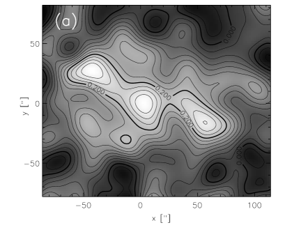
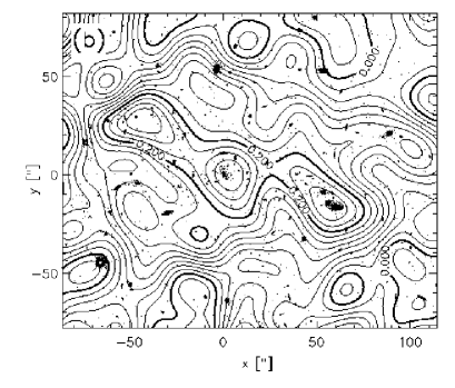
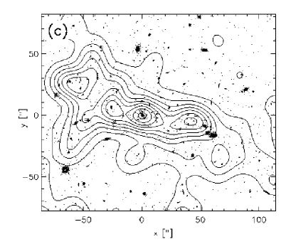
Fig. 18.—: (a) Gray scale image of the mass reconstruction of the central 3.3 by 2.7 arcminute region of the HST mosaic; (b) Overlay of the mass map on the $F814W$ image of MS 1054-03; (c) Overlay of the smoothed light map and the $F814W$ image. All images have been smoothed using a Gaussian filter with a FWHM of 20 arcsec. The interval between adjacent contours is 0.025 in $\kappa$. Comparison of the mass reconstruction with the light distribution shows that there is a fair agreement between the distributions of mass and light.

A robust method to examine the cluster galaxies is to measure the average tangential distortion around an ensemble of cluster members. The results are not very sensitive to the precise cluster mass distribution, provided one confines the analysis to small radii. Due to the clustering of the lenses, the signal at large radii is dominated by the smooth cluster signal. When measuring the signal out to large radii, a careful removal of the cluster signal is required. We subtracted the contribution of the smooth cluster mass distribution from the observed distortion using the two-dimensional mass reconstruction, and computed the shear $\gamma$ taking the $(1-\kappa)$ correction into account.

We used a sample of galaxies brighter than $F814=24.5$ $(\sim 0.05L_{*})$, with colours close to the cluster colour-magnitude relation to study the masses of the cluster galaxies. To minimize the effect of the large scale cluster mass distribution, we excluded galaxies near the centres of the three clumps, resulting in a sample of 241 galaxies. In total, 4300 cluster galaxy-background galaxy pairs were used to measure the distortion.

Massive galaxies produce a larger distortion than less massive galaxies and therefore we normalized the amplitudes of the signals from the various galaxies correspondingly. To do so, we assumed that the shear $\gamma\propto\sigma^{2}\propto\sqrt{L_{B}}$, i.e. we assumed a Faber-Jackson scaling relation. The results are presented in figure 11.

A fit of a singular isothermal model to the data, yielded a detection of the lensing signal at the 99.8% confidence limit. We found for the Einstein radius of an $L_{*}$ galaxy (${\rm L}_{*B}=8\times 10^{10}h_{50}^{-2}{\rm L}_{B\odot}$ for MS 1054-03) a value of $r_{\rm E}=0.26\pm 0.09$ arcseconds, which corresponds to a velocity dispersion of $\sigma=203\pm 33$ km/s. The mass-to-light ratio within a radius of $20h_{50}^{-1}$ kpc is ${\rm M}/{\rm L}_{B}=7.5\pm 2.4h_{50}{\rm M}/{\rm L}_{B\odot}$. Correcting this result for luminosity evolution yields ${\rm M}/{\rm L}_{B}=17\pm 5h_{50}{\rm M}/{\rm L}_{B\odot}$.

If we neglect the effect of the smooth cluster contribution, we find a slightly higher mass for the galaxies: $\sigma=212\pm 32$ km/s. This indicates that the mass estimate determined using the direct averaging method is indeed robust.

Natarayan & Kneib (1998) studied the halo properties of the cluster galaxies in AC 114. They used a maximum-likelihood analysis to constrain the mass and the extent of the galaxy halos. Constraining the extent of the halos of the cluster galaxies in MS 1054 is a delicate task which has not been attempted here. It requires a careful analysis of the smooth cluster mass distribution in a maximum likelihood analysis.

11 Conclusions

We have measured the weak gravitational lensing of faint, distant galaxies by MS 1054-03, a rich cluster of galaxies at $z=0.83$. The data consist of a two-colour mosaic of 6 interlaced images taken with the WFPC2 camera on the Hubble Space Telescope.

The expected lensing signal is low for high redshift clusters, and most of the signal comes from small, faint galaxies. Compared to ground based observations, these galaxies are much better resolved in HST observations. High number densities of sources are reached, and the correction for the circularization by the PSF is much smaller. This enables us to measure an accurate and well calibrated estimate of the lensing induced distortion of the faint background galaxies.

Several effects complicate an accurate analysis when the distortions or the surface density are non-neglegible (e.g. in the cluster cores). We do not measure the shear, but the distortion $g$. Neglecting the effect of a non-zero surface density results in an overestimate of the lensing signal. Furthermore, the method used (KSB95; LK97) underestimates the distortion when it is larger than $\sim 0.3$. Although we correct for these effects, it is best to restrict the analysis to the weak lensing regime, where the convergence $\kappa$ is low, and the distortions are small.

Fig. 19.—: (a) Average tangential shear around an ensemble of cluster galaxies. The signal induced by the smooth cluster mass distribution is removed from the observed signal, using the mass reconstruction. The signal for each lens galaxy has been scaled to match the signal for a $L_{*}$ ($L_{*B}=8\times 10^{10}h_{50}^{-2}L_{B\odot}$) galaxy, assuming that mass scales with $\sqrt{L}_{B}$. The solid line is a singular isothermal sphere fitted to the measured points. It corresponds to a velocity dispersion of $\sigma=203\pm 33$ km/s. (b) Average tangential shear around the cluster galaxies when the phase of the shear is increased by $\pi/2$.

Converting the lensing signal into a mass estimate requires knowledge of the redshift distribution of the faint sources. We have explored the use of photometric redshift distributions inferred from the Northern (Fernández-Soto et al. 1999) and Southern (Chen et al. 1998) Hubble Deep Fields. Comparison of the results for the two fields suggest field to field variations which lead to a 10% systematic uncertainty in the mass estimate for MS 1054-03. Our results for the mass and mass-to-light ratio of MS 1054-03 agree well with other estimators, suggesting that these photometric redshift distributions are a fair approximation of the true distribution. This gives us confidence that we are able to measure a well calibrated weak lensing mass for this high redshift cluster.

Using the $\zeta_{c}$ statistic (Clowe et al. 1998), we find a mass $(1.2\pm 0.2)\times 10^{15}h_{50}^{-1}{\rm M}_{\odot}$ within an aperture of 1 $h_{50}^{-1}$ Mpc radius. Under the assumption of an isothermal mass distribution, this corresponds to a velocity dispersion of $1311^{+83}_{-89}$ km/s. A fit of an isothermal sphere model to the observed tangential distortion at large radii, yields a velocity dispersion of $1365\pm 84$ km/s. However, this result depends on the assumed radial surface density profile. The uncertainties in the mass estimates only reflect the contribution from the intrinsic ellipticities of the sources. The weak lensing mass estimate is in good agreement with the X-ray estimate from Donahue et al. (1998) and the observed velocity dispersion (Tran et al. 1999; van Dokkum 1999).

The observed average mass-to-light ratio in the passband corrected $B$ band is $124\pm 17h_{50}{\rm M}_{\odot}/{\rm L}_{B\odot}$ (measured within a 1 $h_{50}^{-1}$ Mpc radius aperture). We use the results from van Dokkum et al. (1998) to correct our estimate for luminosity evolution. The resulting mass-to-light ratio of $269\pm 37~{}h_{50}{\rm M}_{\odot}/{\rm L}_{B\odot}$ can be compared to results obtained for nearby clusters, and is in excellent agreement with the findings of Carlberg et al. (1997).

Our high resolution mass reconstruction shows three distinct peaks in the mass distribution, which are in good agreement with the irregular light distribution. The results of LK97 lacked the resolution to detect this substructure. In projection the clumps are approximately 500 $h_{50}^{-1}$ kpc apart, and we estimate the timescale for virialization to be at on the order of $\sim$ 1 Gyr. Thus the cluster should be virialized at a redshift $z\sim 0.65$. We found that the clumps are of roughly equal mass, with corresponding velocity dispersions of $\sim 700$ km/s.

To study the masses of the cluster members, we have measured the average tangential shear around a sample of 241 bright cluster galaxies. Assuming the Faber-Jackson scaling relation we find a velocity dispersion of $203\pm 33$ km/s for an $L_{*}$ galaxy (${\rm L}_{*B}=8\times 10^{10}h_{50}^{-2}{\rm L}_{B\odot}$ for MS 1054-03). The mass-to-light ratio within a radius of $20h_{50}^{-1}$ kpc is ${\rm M}/{\rm L}_{B}=7.5\pm 2.4h_{50}{\rm M}/{\rm L}_{B\odot}$. Correcting this result for luminosity evolution yields ${\rm M}/{\rm L}_{B}=17\pm 5h_{50}{\rm M}/{\rm L}_{B\odot}$.

The number of known massive high redshift clusters of galaxies is increasing rapidly. The results presented here demonstrate that these systems can be studied with sufficient signal-to-noise to be of interest for studies of cluster formation. The improved sampling and throughput of the Advanced Camera for Surveys, that will be installed on the HST in the near future, will be very useful for weak lensing analyses of high redshift clusters of galaxies, especially when the results are combined with forthcoming X-ray observations. The combination of detailed weak lensing analyses and X-ray observations by Chandra and XMM will provide important information on the thermodynamics of cluster formation.

The authors thank Pieter van Dokkum for making the data available in reduced form, which has been invaluable for this analysis.

APPENDIX

A Error analysis

The weak lensing signal is obtained by averaging the shape measurements of a number of faint galaxies. The noise in the shape estimate differs from object to object, and therefore it is important to weight the measurements properly. For bright galaxies the error on the shear measurement is dominated by the intrinsic ellipticity distribution of the galaxies. At fainter magnitudes, shot-noise increases the uncertainty in the measurements. As these galaxies require large seeing corrections, the measurement error on the distortion can be quite high. This is illustrated in figure A.1. Figure A.1a shows the observed scatter in the polarization as a function of apparent magnitude in the $F814W$ band. As fainter objects suffer more from the circularization by the PSF one would expect the scatter to decrease towards fainter magnitudes. However, the increasing contribution by shot noise (indicated by the solid line) cancels out the effect of the circularization. Figure A.1b shows the observed scatter in the ellipticities (shear) of the objects. The scatter at faint magnitudes increases rapidly due to the combination of shot noise and large PSF corrections. The solid line indicates the expected scatter due to the combination of shot noise and PSF correction. We estimate the weighted mean of the distortion using:

$$\langle g_{i}\rangle=\frac{\sum w_{n}e_{i,n}/P^{\gamma}_{n}}{\sum w_{n}},$$ (A1)

where the weight $w_{n}$ is the inverse of the variance of the distortion:

$$w_{n}=\frac{1}{\sigma_{g}^{2}}=\frac{P_{\gamma}^{2}}{\langle\gamma_{0}^{2}\rangle P_{\gamma}^{2}+\langle\Delta e^{2}\rangle},$$ (A2)

where $\langle\gamma_{0}^{2}\rangle$ is the scatter due to the intrinsic ellipticity of the galaxies, $P_{\gamma}$ is the pre-seeing shear polarizability and $\langle\Delta e^{2}\rangle^{1/2}$ is the error estimate for the polarization, which is derived below. This procedure, however, gives only the optimal estimate for the average ellipticity, but does not account for the fact that the nearby bright galaxies are lensed less efficiently than faint high redshift galaxies. To get the best lensing estimate it is therefore also necessary to weight with $\beta$ as well. This is demonstrated in figure A.1a, where we show the weight function as a function of apparent magnitude (solid line). The dashed line shows the weight function hen we include the strength of the lensing signal. This effectively decreases the weight of bright (nearby) galaxies and increases the relative weight of the faint (distant) galaxies. It is also interesting to see which magnitude range contributes most to the measurement of the distortion. In figure A.1b we plot the weight function for each magnitude bin times the number of galaxies in that bin. This gives the total contribution of each bin to the measurement of the distortion. Although the bright galaxies have the highest weight function (cf. figure A.1a), they are not so numerous to contribute significantly to the lensing signal. At the faint end both incompleteness and increasing noise causes the contribution to decrease rapidly. Figure A.1b also shows that including the strength of the lensing signal $(\beta)$ changes the profile only slightly. It shows that galaxies with $F814W$ magnitudes between 24 and 26.5 contribute most to the lensing signal.

A.1 Estimating the measurement error on the polarization

Here we derive an expression to estimate the error on the polarization measurement, using the observations. The observed quadrupole moments are given by:

$$I_{ij}^{\rm obs}=\int d^{2}xx_{i}x_{j}W(\vec{x})f_{\rm obs}(\vec{x}),$$ (A3)

which are combined to form the two-component polarization.

$$e_{1}=\frac{I_{11}-I_{22}}{I_{11}+I_{22}}~{}{\rm and}~{}e_{2}=\frac{2I_{12}}{I_{11}+I_{22}}$$ (A4)

Due to noise, the true image $f_{\rm true}(\vec{x})$ is changed to the observed image $f_{\rm obs}(\vec{x})$:

$$f_{\rm obs}(\vec{x})=f_{\rm true}(\vec{x})+\sigma b(\vec{x})+d(\vec{x})\sqrt{f(\vec{x})},$$ (A5)

where we take $\langle b(\vec{x})^{2}\rangle^{\frac{1}{2}}=\langle d(\vec{x})^{2}\rangle^{\frac{1}{2}}=1$. The first term in equation A5 gives the true image, the second term is the noise in the background, and the third contribution comes from the shot noise due to the image. We therefore observe quadrupole moments given by:

$$I^{\rm obs}_{ij}=I^{\rm true}_{ij}+\int d^{2}xx_{i}x_{j}W(x)\left(\sigma b(\vec{x})+d(\vec{x})\sqrt{f(\vec{x})}\right)$$ (A6)

As $\langle b(\vec{x})\rangle=\langle d(\vec{x})\rangle=0$, this shows that $\langle I^{\rm obs}_{ij}\rangle=I^{\rm true}_{ij}$. Thus noise does not introduce a bias in the average measurement of the quadrupole moments. However, it does introduce a neglegible bias in the polarization. We now can estimate the variance in the observed Fig. A20.—: (a) Plot of the observed scatter in the polarization as a function of apparent magnitude in the $F814W$ band. The scatter is fairly constant with apparent magnitude. The PSF circularizes the images of the faint galaxies, but the increasing scatter due to shot noise cancels out this effect. (b) Plot of the observed scatter in the ellipticities (shear) of the galaxies. At bright magnitudes the scatter is dominated by the intrinsic ellipticities of the galaxies. At fainter magnitudes the scatter increases rapidly due to increasing shot noise and large PSF corrections. The contribution of the shot noise to the scatter is indicated by the solid line. quadrupole moments using equation A6 and noting that $\langle b(\vec{x})b(\vec{y})\rangle=\langle b(\vec{x})b(\vec{y})\delta(\vec{x}-\vec{y})\rangle$, $\langle d(\vec{x})d(\vec{y})\rangle=\langle d(\vec{x})d(\vec{y})\delta(\vec{x}-\vec{y})\rangle$, and $\langle b(\vec{x})d(\vec{y})\rangle=0$, where $\delta(\vec{x}-\vec{y})$ is the Dirac delta function. This yields:

$$\langle\Delta I_{ij}\Delta I_{kl}\rangle=\int d^{2}xx_{i}x_{j}x_{k}x_{l}W^{2}(\vec{x})\left(\sigma^{2}+f(\vec{x})\right)$$ (A7)

Fig. A21.—: (a) Weight function as a function of apparent $F814W$ magnitude (solid line). For bright galaxies the weight function is dominated by the intrinsic ellipticities of the galaxies. At fainter magnitudes, the weight function decreases rapidly due to the increasing measurement error on the distortion. Including the strength of the lensing signal ($\beta$) yields a different weight function (dashed line), which lowers the weight of bright (nearby) galaxies and thus increases the relative weight of faint (distant) galaxies. (b) Plot of the weight function times the number of objects in each magnitude bin as a function of apparent $F814W$ magnitude (solid line). This plot shows which magnitude bin contributes most to the signal. Although bright galaxies have the highest weight (cf. figure A.1), they are not so numerous that they contribute significantly to the lensing signal. Including the strength of the lensing signal $(\beta)$ changes the profile mainly at the bright end, but the differences are small. The lensing signal is dominated by galaxies with $F814W$ magnitudes between 24 and 26.5.

We now want to estimate the errors on the measurements of the polarizations $e_{1}$ and $e_{2}$ and express them in terms of the errors on the quadrupole moments. This finally gives:

Fig. A22.—: Left panel: Ellipticity introduced by constructing an interlaced images from images with imperfect offsets. The reference star (a Tiny Tim PSF) is centered exactly on a pixel. This image is shifted $(\Delta x,\Delta y)$ and an interlaced image is created, assuming the shift was (0.5, 0.5) pixel; Right panel: The same procedure was repeated for the case in which the reference star is placed at the intersection of four pixels. The sticks indicate the direction and the size of the introduced ellipticity. If the shifts are half pixel, the measured ellipticity is correct. The offsets of our observations for $F814W$ (open circles) and $F606W$ (solid triangles) are also indicated. For one $F814W$ pointing the offset is such that results of the interlaced images are biased.

$$\langle\Delta e_{1}^{2}\rangle = \frac{1}{(I_{11}+I_{22})^{2}}[(1-e_{1})^{2}\langle\Delta I_{11}^{2}\rangle+(1+e_{1})^{2}\langle\Delta I_{22}^{2}\rangle$$ (A8)

$$\qquad-2(1-e_{1}^{2})\langle\Delta I_{12}^{2}\rangle]$$

and

$$\langle\Delta e_{2}^{2}\rangle = \frac{1}{(I_{11}+I_{22})^{2}}[e_{2}^{2}(\langle\Delta I_{11}^{2}\rangle+\langle\Delta I_{22}^{2}\rangle)$$ (A9)

$$\qquad+(4+2e_{2}^{2})\langle\Delta I_{12}^{2}\rangle$$

$$\qquad-4e_{2}(\langle\Delta I_{11}\Delta I_{12}\rangle+\langle\Delta I_{22}\Delta I_{12})\rangle].$$

From simulations and real images we find that the errors on both $e_{1}$ and $e_{2}$ are similar. This estimate for the error on the polarization can be calculated from the observations and allows us to properly weight the signals of the galaxies using equation A2.

B The effects of interlacing

The images of small, faint galaxies in WFPC2 observations are poorly sampled. HFKS98 showed that as a result the smallest objects cannot be corrected reliably for the PSF effects. However, several techniques can be used to improve the sampling of WFPC2 observations by dithering the exposures (Fruchter & Hook 1998). When the shifts are half pixel in both $x$ and $y$ (modulo integer pixel shifts) one can construct an interlaced image (Fruchter & Hook 1998) which has a $\sqrt{2}$ better sampling. Interlaced images were constructed from the observations of MS 1054-03. Doing so, we assumed that the offsets were exactly half pixel. Due to pointing errors and the camera distortion the real offsets are slightly different.

Fig. B23.—: Ellipticity introduced by imperfect offsets and WFPC2 camera distortion. (a): The introduced ellipticities for the worst offset in the $F814W$ filter $(\Delta x,\Delta y)=(5.71,5.89)$ as a function of position. In this case it is clear that interlacing introduces a bias in the observed shapes, and therefore these data (the $F814W$ image of the first pointing) are not used in the weak lensing analysis. (b): The introduced ellipticity for the second worst offset (5.53, 5.60). In this case the bias is very small. Due to the telescope distortion the effect is somewhat larger at the edges of the chips. The sticks indicate the direction and the size of the introduced ellipticity.

In this section we examine the effect of imperfect offsets on the shape measurements. To do so, we examine the change in the shape of a model PSF. Although interlacing is not a convolution, it affects large objects (as these are well sampled even before interlacing) less than small objects. By examining the effects on the PSF, we study a worst case scenario. The effects should be less for most of the galaxies used in the weak lensing analysis. We use a ten times oversampled model PSF calculated using Tiny Tim. This PSF is shifted and rebinned to WFPC2 sampling and convolved with the pixel scattering function, in order to realistically mimic the WFPC2 PSF. We start with a reference image in which the star is centered exactly on a pixel. This image is shifted $(\Delta x,\Delta y)$ and an interlaced image is created assuming the shift was exactly (0.5, 0.5) pixels. The resulting image is analysed and the measured ellipticities are compared to the correct value. The change in ellipticity as a function of the applied offset is presented in figure A22 (left panel). When the reference star is placed at the intersection of four pixels the results are different, as is indicated in figure A22 (right panel). These two extreme cases should cover the full range of possible configurations. In figure A22 we also plot the observed offsets for our data. The open circles represent the offsets of the $F814W$ images, and the solid triangles show the offsets for the $F606W$ images. Only one $F814W$ pointing has such a deviating offset that the shape measurements cannot be used for our weak lensing analysis. In all other images the offsets are such that no significant bias is introduced by the interlacing. Even if the offset is perfect in the centre of the image, telescope distortions will result in imperfect offsets at the edges. We simulated the amplitude of the effect using the coefficients for the telescope distortions from Holtzman et al. (1995). Figure B23 shows the introduced ellipticity for our worst offset (5.71, 5.89). The bias in the observed ellipticities is clear in this case. These data (the $F814W$ image of the first pointing) were not used in the weak lensing analysis. The second worse offset (5.53, 5.60) is also shown in this figure. The ellipticity introduced in this case is small. Only at the edges of the chips the camera distortion introduces a small effect. As the effect is even smaller for galaxies, we feel certain that we can use the interlaced images for our weak lensing analysis.

References

- Bahcall & Fan Bahcall, N.A., & Fan, X. 1998, ApJ, 504, 1
- Bertin & Arnouts Bertin, E., & Arnouts, S. 1996, A&AS, 117, 393
- Binggeli Binggeli, B., Sandage, A., & Tammann, G.A. 1988, ARA&A, 26, 509
- Brainerd et al. 1996 Brainerd, T.G., Blandford, R.D., & Smail, I. 1996, ApJ, 466, 623
- Broadhurst et al. 1995 Broadhurst, T. J., Taylor, & A. N., Peacock, J.A. 1995, ApJ, 438, 49
- Burstein & Heiles 1982 Burstein, D., & Heiles, C. 1982, AJ, 87, 1165
- Castander et al. 1994 Castander, F., Ellis, R., Frenk, C., Dressler, A., & Gunn, J. 1994, ApJ, 424, L79
- Carlberg et al. 1997 Carlberg, R.G., Yee, H.C., & Ellingson 1997, ApJ, 478, 462
- Chen et al. 1998 Chen, H.-W., Fernández-Soto, A., Lanzetta, K.M., Pascarelle, S.M., Puetter, R.C., Yahata, N., & Yahil, A., preprint, astro-ph/9812339 http://www.ess.sunysb.edu/astro/hdfs/home.html
- Clowe et al. 1998 Clowe, D., Luppino, G.A., Kaiser, N., Henry, J.P., & Gioia, I.M. 1998, ApJ, 497, L61
- Donahue et al. 1998 Donahue, M., Voit, G.M., Gioia, I., Luppino, G.A., Hughes, J.P., & Stocke, J.T. 1998, ApJ, 502, 550
- Ebeling et al. 1999 Ebeling, H., Jones, L.R., Perlman, R., Scharf, C., Horner, D., Wegner, G., Malkan, M., & Mullis, C.R. 1999, submitted to ApJ
- Eke 1996 Eke, V.R., Cole, S., & Frenk, C.S. 1996, MNRAS, 282, 263
- Gunn et al. 1986 Gunn, J., Hoessel, J., & Oke, J.B. 1986, ApJ, 306, 30
- Fahlman et al. 1994 Fahlman, G., Kaiser, N., Squires, G., & Woods, D. 1994, ApJ, 431, L71
- Fernandez-Soto etal. Fernández-Soto, A., Lanzetta, K.M., & Yahil, A. 1999, ApJ, 513, 34
- Fruchter and Hook 1998 Fruchter, A.S., & Hook, R.N. 1998, preprint, astro-ph/9808087
- Gioia et al. 1990 Gioia, I.M., Maccacaro, T., Schild, R.E., Wolter, A., Stocke, J.T., Morris, S.L., Henry, J.P. 1990, ApJS, 72, 567
- Gioia & Luppino 1994 Gioia, I.M., & Luppino, G.A. 1994, ApJS, 94, 583
- Gioia et al. 1998 Gioia, I.M., Henry, J.P., Mullis, C.R., Ebeling, H., & Wolter, A. 1998, AJ, accepted
- Gorenstein et al. 1988 Gorenstein, M.V., Shapiro, I.I., & Falco, E.E 1988, ApJ, 327, 693
- Holtzman et al. 1995 Holtzman, J.A., Hester, J.J., Casertano, S., Trauger, J.T., Watson, A.M., et al. 1995, PASP, 107,156
- Henry et al 1997 Henry, J.P., Gioia, I.M., Mullis, C.R., Clowe, D.I., Luppino, G.A., Boehringer, H., Briel, U.G., Voges, W., & Huchra, J.P. 1997, AJ, 114,1293
- Hoekstra et al. 1998 Hoekstra, H., Franx, M., Kuijken, K., & Squires, G. 1998, ApJ, 504, 636 (HFKS98)
- Jorgensen et al. 1995 Jørgensen, I., Franx, M., & Kjaergaard, P. 1995, MNRAS, 273, 1097.
- Kaiser & Squires 1993 Kaiser, N., & Squires, G. 1993, ApJ, 404, 441
- Kaiser, Squires & Broadhurst 1995 Kaiser, N., Squires, G., & Broadhurst, T. 1995, ApJ, 449, 460
- Kelson et al. 1997 Kelson, D.D., van Dokkum, P.G., Franx, M., Illingworth, G.D., & Fabricant, D. 1997, ApJ, 478, L13
- Kuijken Kuijken, K. 1999, A&A, in press (astro-ph/9904418)
- Luppino & Kaiser 1997 Luppino, G.A., Kaiser, N. 1997, ApJ, 475, 20 (LK97)
- Mellier 1999 Mellier, Y. 1999, preprint, astro-ph/9812172
- Neumann et al. 1999 Neumann, D., Arnoud, M., Joy, M., & Patel, S.K. 1999, in preparation
- Postman et al. 1998 Postman, M., Lubin, L.M., & Oke, J.B. 1998, AJ, 116, 560
- Rhodes et al. 1999 Rhodes, J., Refregier, A., & Groth, E. 1999, preprint, astro-ph/9905090
- Rosati et al. 1998 Rosati, P., Della Ceca, R., Norman, C., & Giacconi, R. 1998, ApJ, 492, L21
- Schneider & Rix 1997 Schneider, P., & Rix, H.-W. 1997, ApJ, 474, L25
- Seitz & Schneider 1997 Seitz, C., & Schneider, P. 1997, A&A, 318, 687
- Smail et al. 1994 Smail, I., Ellis, R., Fitchett, M., & Edge, A. 1994, MNRAS, 270, 245
- Squires & Kaiser 1996 Squires, G. & Kaiser, N. 1996, ApJ, 473, 65
- Tyson et al. 1990 Tyson, J.A., Wenk, R.A., & Valdes, F. 1990, ApJ, 349, L1
- Tran et al. 1999 Tran, K.-V. H., Kelson, D.D., van Dokkum, P.G., Franx, M., Illingworth, G.D., & Magee, D. 1999, preprint, astro-ph/9902349
- Van Dokkum 1999 van Dokkum, P.G. 1999, PhD Thesis, Groningen University
- Van Dokkum & Franx 1996 van Dokkum, P.G., & Franx, M. 1996, MNRAS, 281, 985
- Van Dokkum et al. 1999 van Dokkum, P.G., Franx, M., Kelson, D.D., & Illingworth, G. 1998 ApJ, ApJ, 504, L17
- Van Dokkum et al. 1998 van Dokkum, P.G., Franx, M., Fabricant, D., Kelson, D.D., & Illingworth, G. D 1998, ApJ, preprint, astro-ph/9906152
- Williams et al. 1996 Williams, R.E., et al. 1996, AJ, 112, 1335
- Willick 1999 Willick, J.A. 1999, preprint, astro-ph/9904367