Excesses of faint galaxies around seven radio QSOs at 1.0$<z<$1.6

Abstract

We have conducted an optical study of the environments of seven radio-loud quasars at redshifts $1<z<1.6$. In this paper we describe deep $B$ and $R$ band images obtained for fields of $\sim$6$\times$6 arcmin around these quasars with 3$\sigma$ limiting magnitudes of $B\sim 26$ and $R\sim 25.4$. We found an statistically significant excess of faint ($B>22.5$ and $R>22.0$) galaxies on scales of $r<$170” and $r<$35” around the quasars. The number of excess galaxies, their magnitudes and the angular extension of the excesses are compatible with clusters of galaxies at the redshift of the QSOs. We also found that the quasars of our sample are in general not located at the peak of the density distribution, lying in a projected distance of about $\sim$70” from it. This result agrees with the scenario of a link between overdensities of galaxies around radio sources and the origin of their radio emission.

1 Introduction

Evidence has been accumulating over the last decade that there is a link between quasar activity and the environment of the host galaxy (e.g., Stockton 1982; Yee & Green 1984, 1987; Gehren et al. 1984; Hutchings et al. 1984; Hintzen 1984; Yee 1987; Ellingson et al. (1991); Hintzen et al. (1991); Yee & Ellingson (1993); Fisher et al. (1996);Yamada et al. (1997); Hall et al. (1998); Hall & Green (1998)). In particular, the galaxy-galaxy interaction appears to play a substantial role as the triggering or fuelling mechanism of the nuclear activity. The large fraction of host galaxies (HG) of radio-loud quasars undergoing tidal interactions/merging processes (e.g. Disney et al. 1995; Hutchings & Neff 1997), the high absolute magnitudes of these galaxies (e.g. Carballo et al. 1998, and references therein), and the velocity distribution of galaxies around the QSOs (Heckman et al. 1984; Ellingson et al. (1991)) lend support to this scenario (Yee & Ellingson (1993)).

Furthermore, Yee & Green (1987), Ellingson et al. (1991) and Yee & Ellingson (1993) presented strong evidence of a link between radio emission and clustering of galaxies around QSOs. They found that there are significant differences between the environments of radio-loud and radio-quiet quasars. While radio-loud quasars are associated with clusters of galaxies of Abell richness class 0-2, radio-quiet quasars inhabit environments of Abell richness class poorer than 0.

These results are based on searches of overdensities around low-redshift quasars ($z\leq$0.7). At higher redshifts the number of studies are scarce, or they are focused in one or a few objects (Hintzen et al. 1991; Boyle & Couch 1993, Hutchings et al. 1993, Yamada et al. 1997, Hall & Green 1998). It seems that the dichotomy of radio-loud/radio-quiet environment extrapolates to higher redshifts. Hintzen et al. (1991) reported on the observation of 16 fields around radio-loud QSOs with $0.9\leq z\leq 1.5$. Their sample was selected as radio-loud quasars from the Véron-Cetty & Véron (1984) catalog. They found a significant excess of galaxies within a radius of 15 arcsec around the quasars. However, Boyle & Couch (1993) found no excess of galaxies around their sample of 27 radio-quiet quasars, at the same redshift.

Hall et al. (1998) and Hall & Green (1998) have recently reported on an excess of faint galaxies ($K\geq$19) around a sample of 31 radio-loud quasars, covering a redshift range $z$=1-2. Although the sample was observed at the optical and NIR wavelengths, the excess was found in their $K$-band images. The excess occurs on two spatial scales: a peak at $\theta<$35” from the quasars and a smooth component down to $\theta\sim$100”, which is the largest scale sampled by their $K$-band images. The magnitudes and colors of the excess galaxies are consistent with a population of early-type galaxies at the quasar redshift. This excess is stronger for the more radio-powerful and steep-spectrum radio-quasars, and it is consistent with a cluster of galaxies with Abell richness class $\sim 1.5\pm 1.5$.

It is still an open question whether the most important factor affecting the evolution of radio-loud QSOs in clusters is the absolute density of the environment, the density within $\sim$0.5Mpc, or even the conditions in the host galaxy and any galaxies interacting with it (Hall & Green 1998). It is important to determine if clusters around quasars at high-$z$ are really embedded in large-scale overdensities, or if they are young, less-peaked, smoothed clusters that extend to large scales ($\sim$2-3Mpc). Paraphrasing Hall & Green (1998) “…larger areas (4’$\times$4’) around our sample need to be imaged to confirm the large-scale ($\theta\sim$100”) galaxy excess around z=1-2 radio-loud quasars and to determine the true angular extent of this excess…”.

In this paper we report on the results obtained from deep CCD imaging survey of the fields around 7 radio-quasars selected from the B3-VLA quasar sample (Vigotti et al. 1997), in the redshift range $1<z<1.6$. The quasars are steep-spectrum radio-sources and they have been selected as the brightest ones of this sample at this $z$ range ($\langle z\rangle\sim 1.4$), using the available optical information when the selection was made (Vigotti et al. 1997). New optical observations show that it is not true any longer (Carballo et al. 1999), but they are still on the range of the brightest ones, having $\langle M_{\rm B}\rangle\sim-26.6$. The size of the images (6’$\times$6’) will allow us to sample the density of galaxies to scales down to $\sim$190”. In Sect. 2 we describe the observations and data analysis. In Sect. 3 we analyse the possible projected clusters around the QSOs, describing some of their properties. In Sect. 4 we compare with previous results, and discuss about possible interpretations. The conclusions are presented in Sect. 5. Throughout this paper we adopt $H_{0}$=50 km s^-1Mpc^-1 and q₀=0.5 .

2 Observation and data processing

Observations were carried out during the night of 1997 March 13 at the Cassegrain focus of the 2.2m Telescope at Calar Alto (Spain). $B$ and $R$ standard Johnson’s filters were used and the pixel scale was 0.533 arcsec$\cdot$pixel^-1. The field of view corresponds to $\sim$6${}^{\prime}\times 6^{\prime}$ in all the images. The seeing was $\sim$1.6”, and variations along the night were lower than 0.2”.

An standard observing procedure was used. CCD bias were measured taking 0 s. exposure time images. Sky flat-fields for each filter were obtained during twilight. Dome-flats were also obtained in order to check the sky flat-fields stability; however, sky flat-fields have been found to work properly and to produce better flat-fielding. In order to reduce the cosmic ray events, and obtain a proper cleaning of them, the following observing procedure was applied: two frames of 900 seconds exposure time at the $R$ band and three frames (two of 900 seconds and another one of 600 seconds) at the $B$ band were obtained for each QSO.

The individual frames were reduced using standard tasks in IRAF¹ package. First, the corresponding bias was subtracted for each image. A flat-field image was obtained for each filter using the average of the sky flats with higher signal-to-noise and without saturated pixels. The images were corrected using these flat-fields, and the error produced by this correction was lower than 0.8%. Cosmic ray events in each frame were detected and replaced by the average of the neighbours using the COSMICRAYS task on IRAF packages.

The final images, with 1800 and 2400 seconds exposure time for the $R$ and $B$ band respectively , were obtained by coadding the reduced individual frames for each object and filter.

2.1 Photometric calibration

Flux calibration for each night and filter was carried out by a standard procedure using 28 Landolt faint photometric standard stars (Landolt 1992, and references therein), that were observed for each filter along the night. The extinction coefficient and zero-point were obtained by a least-square fitting between the instrumental magnitude ($-2.5\cdot{\rm log}_{\rm 10}(N_{c}/t)$, where $N_{c}$ is the number of counts), and the air-mass ($X$). The night was photometric, and the $rms$ of these least-square fits were 0.086 and 0.027 for the $B$ and $R$ band respectively.

The QSO magnitudes were measured on the images using circular apertures centred at the emission peak. The aperture radius was fixed for the seven QSOs to 6.4”, and it was set to the value at which the intensity of the object reached the background for the QSO with the larger seeing image. Table 1 lists a summary of these results, including some useful radio properties of the quasars and their redshifts. Carballo et al. (1999) report on the optical photometry of 73 B3-VLA quasars. They observed the seven objects of our sample, in both the $B$ and $R$ band, and quote magnitudes consistent with those reported here, within an error of $\sim$0.1 mag.

Table 1: QSOs sample

B3 Name $$z$$ ^a

0740+380C 1.063 -1.29 7.88 18.360.09 17.650.03

0926+388 1.630 -1.09 1.84 19.680.09 19.220.03

1123+395 1.470 -0.82 1.05 18.540.09 17.960.03

1148+387 1.303 -0.94 4.08 17.360.09 16.740.03

1206+439B 1.400 -0.85 14.90 18.410.09 17.390.03

1315+396 1.560 -0.49 3.87 18.700.09 18.280.03

1435+383 1.600 -0.85 1.91 18.230.09 17.830.03

• in $10^{28}$ W Hz^-1

2.2 Data processing and number counts

We searched for galaxies in the frames using the SExtractor package (Bertin & Arnouts (1996)). This program detects and deblends objects using an isophotal threshold above the local sky and produces a catalogue of their properties. This catalogue includes information of position, shape, profile, magnitude and type, for each detected object. Objects are classified using a neural network, which takes as input parameters 8 isophotal areas, the peak intensity and the FWHM (full width at half maximum) of each object. The $seeing$, defined as the FWHM of the stars, is another input parameter. This network determines a “star-like-index”, which is, by definition, 0 for the galaxies and 1 for the stars. In practice, a value of $\sim 0.7$ works fine to separate stars and galaxies.

We selected a detection threshold of 5 connected pixels ($\sim$1.4 arcsec²) above 2$\sigma_{\rm sky}$ level per pixel, which guarantees that $all$ the detected objects have signal-to-noise larger than 4.5. This detection criterium is similar to those reported in previous works. For instance, Hall et al. (1998) used a catalog of objects detected with a minimum area of 1.9 arcsec² and a detection threshold of 5$\sigma$. We note here that for an area of 1.9 arcsec² our detection threshold would be 5.2$\sigma$. We applied SExtractor to the 7 $R$-band and 7 $B$-band images using this detection criterium. After cleaning sources close to the frame borders or near to large foreground galaxies, we obtained the final catalogs for each field and filter. We found that the mean magnitudes of the faintest detected objects in the different fields are $B$=$25.58\pm 0.35$ and $R$=$24.80\pm 0.28$. These are the 4.5$\sigma$ limiting magnitude of our catalogs.

The $3\sigma$ limiting magnitude for 5 connected pixels of the images can be estimated by measuring the standard deviation on the sky. This yields mean values of $B^{3\sigma}_{\rm lim}$=26.0$\pm$0.4 and $R^{3\sigma}_{\rm lim}$=25.4$\pm$0.3. This would imply a 4.5$\sigma$ limiting magnitude of $B^{4.5\sigma}_{\rm lim}$=25.6$\pm$0.4 and $R^{4.5\sigma}_{\rm lim}$=24.9$\pm$0.3, which are consistent with the magnitudes of the faintest detected objects in the catalogs.

The 3$\sigma$ limiting magnitude of the $R$-band images is similar to values previously reported in recent works. Hall & Green (1998) and Hall et al. (1998) reported a $3\sigma$ limiting magnitude of $r\sim$25.5 mag, for a minimum detection area of 1.9arcsec². Taking into account the relation between the Thuan-Gunn $r$-band and the Johnson $R$-band magnitudes ($r=R+0.43+0.15(B-V)$ ; Kent 1985), and assuming a range of $B-V$ colours between 0 and 2 (for typical elliptical galaxies at $0<z<2$), the Hall & Green $3\sigma$ limiting magnitude would be $R\sim$24.8-25.1. These authors study overdensities of galaxies around radio-quasars at $1<z<2$, whereas our maximum redshift is $z\sim$1.6. Therefore we conclude that our images are adequate to search for galaxies around QSOs at these redshifts.

In order to test the validity of our method we have made a set of simulations. Seven simulated images have been built with the same magnitude-to-counts relation, background and noise than the $R$-band images of our sample. The simulated images were built using the ARTDATA tasks in the IRAF package. In each image 1200 galaxies, uniformly spatially distributed, and with a number-counts distribution following a power-law with a slope of 0.4, ranging from $R$=18.0 to 25.5, were simualted. We added 750 stars to each image, with magnitudes in the range 14 to 25 mag, and similar spatial and flux distribution than the galaxies. We have artificially increased the star/galaxy number ratio with respect to that observed in our images in order to test the galaxy detection and classification at faint flux levels.

The whole procedure was applied over these simulated images. The results have been compared with the input parameters of the objects. We found that 85% of the sources were correctly classified down to $R\leq$23.5. The percentage of objects (galaxies+stars) misclassified grows at fainter magnitudes, being around 30% at $R>$23.5. The fraction of galaxies classified as stars is roughly similar to the fraction of stars classified as galaxies. The input number-counts distribution of galaxies was recovered down to $R\leq$23.8 (objects detected up to $\sim$13$\sigma$). A similar result is expected for the objects down to $B<$24.5 mag.

2.2.1 Number counts

A proper determination of the field number-counts and its standard deviation is crucial to detect excesses of galaxies and to quantify their significances. Some authors take the statistical significance using the poissionian standard deviation. But, as have been quoted (Yee & Green 1987, and references therein; Benítez et al. 1995), galaxies tend to cluster, and the true standard deviation depends not only on the number of objects (as in the poissonian case) but also on the two-point correlation function. Therefore, the standard deviation $\sigma(r,N)$ depends on the number of galaxies $N$ and on the angular scale $r$. This is usually expressed as $\sigma(r,N)=\gamma(r)\cdot\sqrt{N}$. The factor $\gamma(r)$ takes account of the angular scale, and since there is no galaxy-galaxy correlations at any scale, it must tend to 1 at some large scale (Yee & Green 1987). The limit $\gamma=1$ corresponds to a poissonian distribution. Ellingson et al. (1991, and references therein) set $\gamma(r)$ to 1.3 for scales of $\sim$60 arcsec, whereas Benítez et al. (1995) found a value of 1.5 for scales as large as $\sim$120 arcsec and Hintzen et al. (1991) assumed a poissonian distribution for scales of $\sim$15 arcsec. We have prefered to make an internal measurement of the factor $\gamma(r)$.

The number of field galaxies in the QSOs images was measured directly and then compared with similar results available in the literature. Two different, and complementary, measurements have been made. First, the number of galaxies in the outer part of the images, in an anulus from $r_{\rm in}$=170” to $r_{\rm out}$=185” around the QSO, was measured in each image. This radius corresponds to $\sim 2.5$ Mpc at the mean redshift of the QSOs and guarantees that there are no contaminations from possible clusters members. The mean galaxy-counts obtained for each QSO field and filter defines a density of field galaxies. The measurement was repeated for different ranges of magnitude, and we obtained a number-counts distribution. This method has the advantage that possible contaminations from the putative cluster members at these scales have been minimized. On the other hand it has the disadvantage that there is only one measurement for each field, and therefore, the standard deviation is not well determined. The measured factor $\gamma$ with this method would correspond to $\gamma(170^{\prime\prime})$.

The second method consists in measuring the number of galaxies in a grid of 25 circular, not overlapping, areas of $35$ arcsec radius ($1.1$ arcmin²). This angular scale corresponds to $\sim$0.5 Mpc at the mean $z$ of the quasars. To minimize contamination from possible clusters, only areas at distances larger than 70 arcsec from the QSOs were considered. This method has the adventage that now we have 16 measurements of the number of field galaxies for each image, resulting in a total of 112 measurements for each band. This provides us with a well determined $\gamma(35^{\prime\prime})$ factor. The major caveat is that it is not possible to guarantee that the areas are not contaminated by cluster members. Recalling that $\gamma(r)\neq 1$ is due to galaxy-galaxy correlations, any clustering would produce an increase of this factor. Therefore, any contamination by cluster members tends to increase the measured value of $\gamma(35^{\prime\prime})$ and to reduce the significance of the possible excess.

Table 2 lists the number of measured field galaxies (we will refer them as expected galaxies throughout this paper, $N_{\rm exp}$) within an area of $\sim$1 arcmin² (a circular area of $r<35$”) at different magnitude ranges, using the two above refereed methods. We also list the computed $N_{\rm exp}$ taken all detected galaxies into account ($B_{\rm all}$ and $R_{\rm all}$ in Table 2). We have re-normalized the number of expected galaxies and its standard deviation to the same area assumming that the distribution of $field$ galaxies is uniform and that the deviation follows the above refereed law ($\sigma$=$\gamma(r)\sqrt{N_{\rm exp}}$). Table 2 also lists the corresponding estimates of the $\gamma$ factor at both scales.

Table 2: Number of expected galaxies within 1.07arcmin² ($r<$35”)

Mag. range N_exp ^a $$\sigma$$/ ^a N_exp ^b / ^b

all 5.882.29 0.95 6.033.27 1.330.26

2.613.57 2.21 2.701.62 0.990.20

1.151.57 1.47 1.011.10 1.100.19

0.280.50 0.95 0.350.59 1.000.13

0.250.42 0.84 0.170.40 1.000.19

0.230.41 0.84 0.070.25 0.950.27

all 8.573.78 1.30 9.093.32 1.100.17

5.085.63 2.50 5.682.33 0.980.26

2.526.33 3.99 2.541.80 1.130.16

1.193.63 3.33 1.011.12 1.110.21

0.641.65 2.06 0.420.75 1.160.22

0.370.61 1.01 0.220.51 1.090.19

• Measured in an anulus of $r_{\rm in}$=170” and $r_{\rm out}$=185”around the QSOs

• Measured in 16 circular areas of $r<$35”

Apparently, there is no significant differences between both measurements, at any band and magnitude range. As expected, the first method gives a lower value of the total expected galaxies (since there is little or no contamination from the cluster), while the second method provides a better value of the standard deviation. The mean value of $\gamma(r)$ is 1.79$\pm$1.05, with the first method, and 1.08$\pm$0.11, with the second one. Both values can not be simply compared, since they have been obtained at different angular scales, but the larger uncertainty of the first one is clear. If $\gamma$ is 1.08 at $r\sim$35”, at larger angular scales its value must be between 1.08 and 1 (the poissonian case). Therefore we will use the number counts derived from the first method and a standard deviation of $1.08\sqrt{N_{\rm exp}}$ for scales larger than or equal to 35”. This value of the $\gamma$ factor at these scales is slightly different from that quoted by Ellingson et al. (1991) who estimated $\gamma\sim 1.3$. We will be comparing our results with those obtained using this value.

As we mention above, this method guarantees little contamination from possible cluster members, but it cannot prevent contamination from large-scale structures. Postman et al. (1998) have noticed that such structures could expand to distances as large as $\sim$6 Mpc (in our adopted cosmology). It is not possible to avoid this problem with present data, since it needs a measurement over several large-scale structure correlation lengths to extimate the ’true’ number-counts. As in the case of ’cluster members’, any large-scale structure contamination will increase the ’real’ expected number counts. Therefore, any overdensity found would be more likely a lower limit, to the extent that the mean density derived from our method is slightly biased upward by the outer extent of the correlated large-scale structure.

Fig. 1 shows the galaxy number-magnitude relation or number-counts distribution for the $R$ and $B$ bands. The slopes of the distributions are $\sim$0.37-0.36 (within the magnitude range 19.0$<R<$23.0) and $\sim$0.49-0.40 (within the magnitude range 19.5$<B<$23.5) respectively. The 100% completeness magnitudes, defined as the magnitude were the number counts drops from a simple power-law, are $R\sim$23 and $B\sim$23.7. These completeness magnitudes correspond to $\sim$30$\sigma$ detections, i.e. photometric errors near to the calibration errors ($\sim$0.03 mag). Both the expected number of galaxies and the slopes obtained are compatible with the results of other authors down to this completeness magnitudes (Metcalfe et al. 1991, Ellingson et al. 1991, Hintzen et al. 1991, Boyle & Couch (1993), Benítez et al. 1995), with variations smaller than $\sim$20%. These small offsets in the number-counts quoted by different authors are mainly due to the different quality of the images (e.g., different seeing and photometric conditions), small differences in the filter transmissions and the use of different methods to detect and classify the objects (e.g., Hintzen et al. 1991, Kron 1980).

Figure 1: The $R$ and $B$-band galaxy number-counts derived from the QSO images.

3 Projected clustering around the QSOs

Since it is not known whether galaxies in the fields of the QSOs are physically associated with them or not, it is not clear which are the optimal magnitude range and angular scale to search for possible excesses. Therefore, we have preferred to use all the available information, measuring the number of galaxies at two different scales around the QSOs, $r_{1}<$170” and $r_{2}<$35”, and at different magnitude ranges. The number of galaxies found around each quasar for each filter band has been added and later compared with the expected number of galaxies. The number of expected galaxies when adding seven fields was obtained using the values listed in Table 2, and were corrected for the corresponding areas and number of fields:

$$N_{\rm exp}^{7fields}(r_{\rm i})=7\cdot(r_{\rm i}/35^{\prime\prime})^{2}\cdot N_{\rm exp}$$

and the corresponding standard deviation is

$$\sigma_{N_{\rm exp}}^{7fields}(r_{\rm i})=\gamma(r_{\rm i})\cdot\sqrt{N_{\rm exp}^{7fields}(r_{\rm i})}$$

where $r_{i}$ is either $r_{1}$ or $r_{2}$.

We have splitted the sample in bins of 1 magnitude down to the above defined “100% completeness magnitude” and an additional bin for galaxies fainter than this magnitude. It is important to note here that all the galaxies, even galaxies fainter than the 100% completeness magnitude ($R>23$ mag, $B>23.7$ mag), were detected up to the 4.5$\sigma$ level. Moreover, the number of expected galaxies was measured in the same images using the same detection/classification procedure as the “excess” galaxies, and, therefore, they are affected by the same incompleteness effects. We define the relative excess (${N-N_{\rm exp}}\over{N_{\rm exp}}$) as $\eta$, and the significance of the excess (${N-N_{\rm exp}}\over{\gamma\sqrt{N_{\rm exp}}}$) as $n\sigma_{\gamma}$.

Table 3 lists the number of detected galaxies at both scales, the number of expected galaxies and the significance of the excess for each band. The significance was computed using $\gamma=$1.08, and also $\gamma=$1.3 by comparison. These values are listed for any range of magnitude, indicated by $all$, and for the above defined bins of magnitude. We found that there is a significant excess of galaxies around the QSOs for both angular scales and filter bands. The significance of the excess ranges from 3.56$\sigma$ for the $B$ band and the largest angular scale, to 4.87$\sigma$ for the $B$ band and the smallest angular scale. The excesses are still significant if we use $\gamma=1.3$. The overdensity is detected both in the $B$ and $R$ bands at a $3-4\sigma$ level, and, therefore, the significance of the detection is larger than if it were detected only in one of the bands. A quadratic propagation of the significance of the excesses in both bands shows that the detection is significant up to 4.60$\sigma$ ($B$+$R$ all in Table 3).

Table 3: Number of galaxies within $r<$170” and $r<$35” from all the fields

Mag. range N_tot N_exp $$n\sigma_{1.3}$$ N_tot N_exp

170” 35”

all 1080 960.82 2.96 3.56 75 41.18 4.05 4.87

all 1569 1398.60 3.51 4.23 97 59.99 3.67 3.83

+ all 4.60 5.53 5.49 6.20

23.5 588 529.9 1.94 2.34 41 23.89 2.69 3.24

23.5 304 241.92 3.07 3.70 20 9.80 2.51 3.02

22.5 123 143.64 -1.32 -1.59 7 5.57 0.46 0.55

21.5 38 31.92 0.82 0.99 4 1.37 1.47 2.09

23.0 604 559.44 1.45 1.74 40 26.25 2.06 2.49

23.0 524 423.36 3.76 4.53 31 17.01 2.61 3.15

22.0 253 219.24 1.75 2.11 17 8.82 2.12 2.55

21.0 110 90.72 1.56 1.87 4 3.71 0.12 0.15

20.0 47 45.36 0.19 0.23 2 1.75 0.15 0.18

The excess presents a tendency with the magnitude range, being significant only for the faintest magnitudes (up to $\sim$3$\sigma$ for $R>22$ and $B>22.5$), for both bands and angular scales. These results indicate that most probably the excess is not due to intervening galaxies, since there is no significant excess down to $R<21$ or $B<22.5$ (see Benítez et al. 1995). The excess galaxies could be physically associated with the QSOs: at the mean redshift of the QSOs ($z\sim 1.4$), galaxies with $R\sim$23 and $B\sim$23.5 would have $M_{\rm R}\sim$-20.9 and $M_{\rm B}\sim$-18.6. A $k$+e correction typical for an E galaxy has been applied, obtained using Bruzual (1983) $c$-model and the GISSEL code (Bruzual & Charlot 1993), assuming a $z_{\rm for}$=5, 1 Gyr of initial burst and a Salpeter mass function (Salpeter 1955), with masses from 0.1 to 125 $M_{\odot}$. These absolute magnitudes are not unusual, and therefore, the galaxies are compatible with being at the quasar redshifts (Bromley et al. 1998; Muriel et al. 1998). Moreover, recent results (Hall & Green 1998) show that galaxies with $r>$23 mag could be associated with quasars at $z\sim$1.5. Taking into account the conversion between $R$ and $r$ magnitudes, their galaxies should have $R>$22.3 mag, being compatible with our result.

The spatial extension of the excesses is also compatible with this interpretation. Fig. 2 shows the radial distribution of the relative excess ($\eta$) with respect to each quasar (in arcsec), for both the $B$ and $R$ band. The mean radial distribution using the seven fields is also shown. The overdensities present a peak down to $\theta\sim$35”-40” in five of the seven fields (at least in one of the two bands). The peak is also visible in the mean distribution of the relative excess. The excess drops smoothly from this peak, and remains flat until $\theta\sim$160”-170”. If the overdensity is due to clusters of galaxies at the redshift of the QSOs ($z\sim 1.4$), the peak would extend to $\sim$350 kpc and the cut-off would be at about $\sim$1500 kpc. These scales are compatible with the physical scales of known clusters at lower redshifts (e.g., Dressler 1980, Ellingson et al. 1991).

The overdensity is produced by $\sim$20-40 galaxies in each field (for both angular scales), which corresponds to low density clusters (Abell richness class between 0-1, Abell 1958 ). Summarizing, the magnitudes, angular sizes and number of galaxies of the excess indicate that most probably we are detecting clusters around the quasars.

Figure 2: Radial distribution of the relative excess of galaxies ($\eta$) with respect to the QSOs (in arcsec) for each quasar field and averaged over all the fields (indicated as $mean$). The thick and thin solid lines correspond to the objects detected in the $R$-band and $B$-band images, respectively.

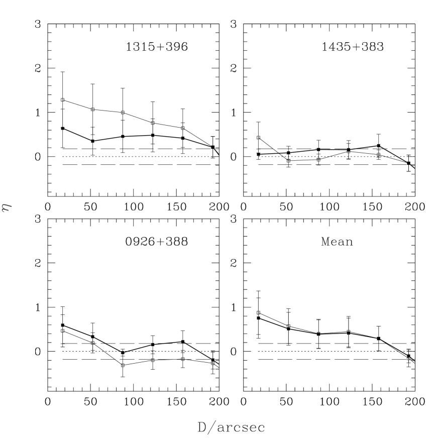
Figure 2: Continued Radial distribution of the relative excess of galaxies ($\eta$) with respect to the QSOs (in arcsec) for each quasar field and averaged over all the fields (indicated as $mean$). The thick and thin solid lines correspond to the objects detected in the $R$-band and $B$-band images, respectively.

3.1 Dependence of excesses with QSO properties

The significance of the excess is at least $\sim$4.6$\sigma$ adding the information from both filters and all the fields. This indicates that the mean significance of the excess, quasar to quasar, must be $\sim$1.7$\sigma$. It is interesting to test if the field-to-field contribution to the total excess is uniform, or it depends on any property of the quasars.

Table 4 lists the number of detected galaxies at $r<35$” from the quasars in each quasar field, together with the significance of the excess (or defect), for each filter band. There are objects where the excess is higher than 4.5$\sigma$, but others present unsignificant deficits. Moreover, although mainly all the quasar fields present a central excess, there are large differences in the spatial distribution of the excess from quasar to quasar (see Fig. 2). This could indicate that there is a dependence of the excess with some property of the quasars.

In order to investigate this possibility we have studied possible correlations between the significance of the excess at $r<35^{\prime\prime}$ and different properties of the radio quasars. No correlation was found between the significance of the excess, $n\sigma_{1.08}$ (of the $B$ and $R$ band and at any angular scale), and redshift, absolute magnitude, $B-R$ colour or radio spectral index of the QSOs. Fig. 3 shows the tendency found between this significance and the radio power of the quasars at 408MHz. The correlation coefficients between both parameters are $r_{\rm xy}$=0.8 for the $R$ band counts, $r_{\rm xy}$=0.4 for the $B$ band, and $r_{\rm xy}$=0.7 for the mean of both (mean without statistic meaning). This tendency could be thought to be due to the large contribution of the B3 1206+439B field, but, removing it, there is still a tendency for the $R$ band counts ($r_{\rm xy}$=0.7). Since our sample is short to be statistically significant this tendency has to be confirmed over larger samples of radio-quasars, but it were expected if there is a connection between radio emission and clustering (Yee & Ellingson (1993), and references therein).

Figure 3: Significance of the relative excess vs. radio power of the quasar. The dotted-line shows the result of a linear least-square fit over the mean significance.

Table 4: Number of galaxies in each field

B3 name $$N_{\rm B}$$

35”

0740+380C 5 -0.34 19 3.29

1148+387 13 2.72 13 1.40

1206+395 18 4.63 21 3.93

1123+387 11 1.95 12 1.09

1315+439B 11 1.95 12 1.09

1435+396 8 0.81 7 -0.50

0926+383 9 1.19 13 1.40

Expected 5.9 8.6

4 Comparison with other results at the same $z$ range

Although there are numerous studies about clustering around QSOs at redshifts lower than 0.9 (Yee & Green (1987), Ellingson et al. (1991), Yee & Ellingson (1993), Fisher et al. (1996), and references therein), the number of studies decreases at higher redshifts (Hintzen et al. 1991, Boyle & Couch 1993, Hall & Green (1998)) or they are focused in one or a few number of fields (Hutchings et al. 1993). At low redshift appears to be clear that radio-loud quasars inhabit groups or clusters of galaxies with an Abell richness class ranging between 0 and 2, and radio-quiet sources inhabit less dense groups of galaxies (e.g., Ellingson et al. (1991)). These results appear to reproduce at high redshift: Hintzen et al. (1991) found a significant excess of galaxies around 16 radio-loud QSOs with 0.9$<z<$1.5 (32 galaxies with $R<$23 within 15 arcsec when the expectation was 19.3), while Boyle & Couch (1993) found no significant excesses around 27 radio-quiet QSOs in the same range of redshifts. This dichotomy may imply a connection between clustering and radio emission (Yee & Ellingson (1993)), which would explain the tendency between relative excess and radio-power found in our sample. Recently, Hall et al. (1998) and Hall & Green (1998) reported their results on optical and NIR observations of a sample of 31 $z$=1-2 radio-loud quasars. They found a significant excess of faint ($K\geq$19) galaxies in these fields, which are compatible with being at the quasars redshifts.

We have found overdensities of galaxies around our radio quasars similar to those reported by Hintzen et al. (1991) and Hall & Green (1998). Hintzen et al. (1991) found that their excess galaxies are $\sim$0.5-0.8 mag brighter than first-ranked galaxies at this redshift, but only if no-evolution is assumed. This result has been used as an argument for the presence of gravitational lensing in these objects (Webster 1991). However, as it has been quoted above, the observed galaxies could be at the redshifts of the QSOs if we take in account a small amount of evolution, like in a E-type galaxy.

Hall & Green (1998) found that the excess increases with power and spectral index of radio-emission. This tendency with spectral index was also recently reported by Mendes de Oliveira et al. (1998). Our results (Sect. 3.1) agree with the first tendency, although we can not test the second one due to the small baseline in radio spectral index of our sample ($\langle\alpha_{408}^{1406}\rangle$=-0.91$\pm$0.25). Hall & Green (1998) also found that the excess was distributed in two different components: a peak within $\theta<$40” from the quasars, and a smooth component along all the covered area. It is necessary to recall here that their results were based on images that allowed to sample the overdensities within $\theta<\sim$100” from the quasars. In Fig. 2, it is possible to see that in almost all our fields the overdensities present a weak peak within $\theta\leq$40” from the quasar, and a smooth component down to $\theta\sim$160”. This structure is present in the averaged distribution (Fig.2). Hall & Green(1998) found that the peak is significant only in $\sim$25% of the fields, although the large-scale overdensity is present in all of them. This is also seen in our sample: only 1148+387 and 1206+439B fields present a strong peak in their central region.

Three different scenarios could explain these results: (1) the quasars inhabit clusters that reside in large-scale overdensities of galaxies, as has been proposed by Hall & Green (1998), (2) they inhabit dynamically young, still not virialized, clusters, which expand smoothly to larger-scales (Ellingson et al. 1991 and Hall & Green 1998), and (3) not all the quasars are at the center of the observed overdensities. This last possibility has not been tested before, and it could easily explain the observed distribution. In fact, only when the overdensity presents a clear peak in the inner region (within $\theta<$40”) it is possible to say that the quasar is roughly at the center of the overdensity.

In order to test this possibility we have estimated the density distribution of galaxies of our $R$-band fields. The density distribution has been calculated using the generalized variable kernel estimate (Silverman 1986) using the Epanechnikov kernel (Epanechnikov 1969). This method is an improvement of the nearest neighbour approach, which adapts the amount of smoothing to the local density of galaxy counts. While the most widely used estimator of the density is based on the number of observations falling in a box of fixed width centred at the point of interest, the kernel estimator is inversely proportional to the size of the box needed to contain a given number of observations (k), and also inversely proportional to a smoothing parameter (h). The number of observations, k, were selected to be roughly the mean density of galaxy counts, and the smoothing parameter was arbitrarily fixed to two points. This density estimate defines better the properties of the distribution than the generally used (see discussion in Silverman 1986).

Fig. 4 shows a contour plot of the density distribution of galaxy counts for each field. The first contour was plotted at the level of the mean density, and the separation between sucessive contours is 1$\sigma$. The position of the quasars in each field was marked as a blue star. It is clearly seen that the quasars are not at the maximum of the distributions, hence, they are not at the “center” of the detected overdensities. The distance between the quasars and the peak of the overdensity range between $\sim$40” and $\sim$100”.

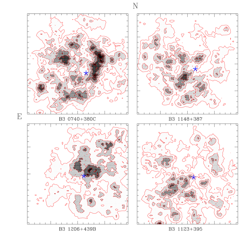
Figure 4: Contour plots of the estimated density distribution of galaxy counts in each field. The first contour corresponds to the mean density, and the separation between sucessive contours is 1$\sigma$. The position of the quasar is marked with a blue star. The distance between small ticks is 20 arcsec.

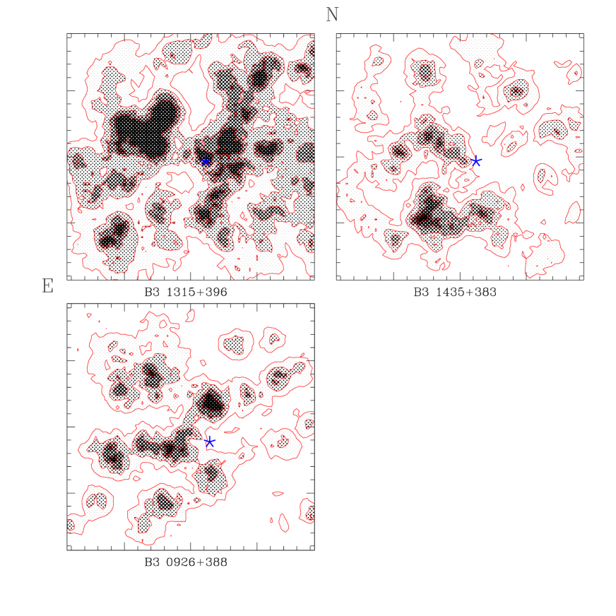
Figure 4: Continued Contour plots of the estimated density distribution of galaxy counts in each field. The first contour corresponds to the mean density, and the separation between sucessive contours is 1$\sigma$. The position of the quasar is marked with a blue star. The distance between small ticks is 20 arcsec.

We have recomputed the radial distributions of the relative excess taking as the origin the “center” of the observed galaxy densities. The result is shown in Fig. 5 for all the quasar fields and for the mean, where the position of the QSOs is indicated with an arrow. It is seen that these excess distributions are more intense at the inner region than the distributions around the quasar positions, and the overdensities within 35” are about twice more significant. In fact, there are fields (e.g. 1435+383) where the smoothness due to the off-centering of the quasar is dramatic (compare Fig. 2 and Fig. 5). In all the fields (except perhaps 1435+383), the quasar is within the overdensity range.

In Fig. 5 it is also seen that the excess still presents a smooth component in some of the quasars fields, although it is less significant than in Fig. 2. Therefore, although the off-centering artificially smooths the radial distribution of relative excess, our result does not completely exclude the other two hypothesis to explain the large scale or smooth component.

Figure 5: Radial distribution of the relative excess of galaxies ($\eta$) with respect to the position of the $center$ of the density (in arcsec) for each quasar field and averaged over all the fields (indicated as mean). The thick and thin solid lines correspond to the objects detected in the $R$-band and $B$-band images, respectively . The arrows mark the position of the quasar in the field.

Figure 5: ContinuedRadial distribution of the relative excess of galaxies ($\eta$) with respect to the position of the $center$ of the density (in arcsec) for each quasar field and averaged over all the fields (indicated as mean). The thick and thin solid lines correspond to the objects detected in the $R$-band and $B$-band images, respectively . The arrows mark the position of the quasar in the field.

5 Summary and conclusions

In this study, the environments of 7 radio-loud quasars at a redshift range between $\sim$1 and $\sim$1.6 have been observed in the $B$ and $R$ band. A significant excess (up to $\sim 3\sigma$) of faint galaxies ($R>$22, $B>$22.5) have been found around them, with magnitudes, angular size of the excess, and number of galaxies all compatible with clusters at the quasar redshifts. This result agrees with previous results on radio-loud quasars at similar redshift ranges (Hintzen et al. 1991, Hall & Green 1998), and it is in contrast with results reported on radio-quiet ones (Boyle & Couch 1993). As at lower redshift ranges, the environments of radio-loud and radio-quiet sources appear to be significantly different (Yee & Green (1987), Ellingson et al. (1991)).

We have found a tendency between radio power and excess of galaxies around QSOs. This trend could be explained by two different mechanisms: (1) If the intracluster gas plays the role of the fuel of the nuclear engine, and radio power is a good estimator of its activity, it is expected that radio power increases with gas density. It is also expected that the amount of intracluster gas were larger in high density clusters, which could explain the correlation; (2) The steep-spectrum extended radio emission is explained by the interaction of $jets$ with the intergalactic medium (e.g. Miley 1980). This medium, with a density of at least $\rho\geq 10^{-28}$ g$\cdot$ cm^-3, confines the radio lobes. It is expected that intergalactic medium were more dense in more populated clusters, and, therefore, there were a connection between cluster population and radio power. Maybe the combination of both mechanisms has to be invoked to explain the proposed tendency. It is interesting to note here that at least the second hypothesis could explain the connection between excess and slope of radio emission found by Hall & Green (1998) and Mendes de Oliveira et al. (1998).

Two possible explanations to the observed link between nuclear activity and environment have been previously proposed: the dynamical state of the cluster galaxies, the evolution of intracluster gas (Yee & Ellingson (1993)). In both schemes the merger or interaction between the host galaxy and companions galaxies plays a substantial role, which reinforces the suggestion that the nuclear activity is triggered by merging processes (Barnes & Hernquist 1992, Shlosman 1994). There are other evidences that support this suggestion, like the large fraction of host-galaxies undergoing tidal interactions/merging process, their large absolute magnitudes, and the velocity distribution of galaxies around quasars (Smith et al. 1986; Hutchings 1987; Disney et al. 1995; Hutchings & Neff 1997; Carballo et al. 1998). Another possible explanation could be a connection between the mass of the central supermassive black hole and the depth of the potential well of the cluster, which could be reflected in the richness of the cluster itself. It is not clear which could be the primary physical cause among the above refereed, and maybe a combination of all of them would be needed to explain the results.

We have found that the quasars of our sample are not located at the center of the clusters. The off-centering of the quasars partially explains the smoothing of the radial distribution of the excess, which apparently shows a two-component distribution (Hall & Green 1998). A better determination of the nature of the overdensity is needed before to present a conclusive explanation for this off-centering. However, this result is not completly unexpected in the framework of merging as the triggering/fuelling mechanism of the nuclear activity: Aarseth & Fall (1980) have shown that the merging process requires that the encounter velocity does not significantly exceed the internal velocity dispersion of the galaxies, approximately 200 km s^-1. Therefore, in virialized cluster cores, galaxy-galaxy merging would be less effective that in the outer part of the clusters, where we have found that the quasars of our sample inhabit.

Among the follow-up research projects suggested by this work, the most important is to select a sample of candidates to cluster members among the galaxies detected in each field. It would be interesting to obtain optical-NIR multiband imaging and multislit spectroscopy of these candidates in order to verify the existence of overdensities at the quasars redshifts, to discriminate the age and metallicity of the selected galaxies, and to do a dynamical study of the putative clusters in order to determine why the active nuclei are not at the center of them.