User Manual for DUSTY

Abstract

DUSTY solves the problem of radiation transport in a dusty environment. The code can handle both spherical and planar geometries. The user specifies the properties of the radiation source and dusty region, and the code calculates the dust temperature distribution and the radiation field in it. The solution method is based on a self-consistent equation for the radiative energy density, including dust scattering, absorption and emission, and does not introduce any approximations. The solution is exact to within the specified numerical accuracy.

DUSTY has built in optical properties for the most common types of astronomical dust and comes with a library for many other grains. It supports various analytical forms for the density distribution, and can perform a full dynamical calculation for radiatively driven winds around AGB stars. The spectral energy distribution of the source can be specified analytically as either Planckian or broken power-law. In addition, arbitrary dust optical properties, density distributions and external radiation can be entered in user supplied files. Furthermore, the wavelength grid can be modified to accommodate spectral features. A single DUSTY run can process an unlimited number of models, with each input set producing a run of optical depths, as specified. The user controls the detail level of the output, which can include both spectral and imaging properties as well as other quantities of interest.

This code is copywrited, 1996–99 by Moshe Elitzur, and may not be copied without acknowledging its origin. Use of this code is not restricted, provided that acknowledgement is made in each publication. The bibliographic reference to this version of DUSTY is Ivezić, Ž., Nenkova, M. & Elitzur, M., 1999, User Manual for DUSTY, University of Kentucky Internal Report, accessible at http://www.pa.uky.edu/$\sim$moshe/dusty.

Make sure that you have the current version, with the latest options and problem fixes, by checking the DUSTY Web site. To be automatically notified of these changes, ask to be placed on the DUSTY mailing list by sending an e-mail to moshe@pa.uky.edu.

1 Introduction

The code DUSTY was developed at the University of Kentucky by Željko Ivezić, Maia Nenkova and Moshe Elitzur for a commonly encountered astrophysical problem: radiation from some source (star, galactic nucleus, etc.) viewed after processing by a dusty region. The original radiation is scattered, absorbed and reemitted by the dust, and the emerging processed spectrum often provides the only available information about the embedded object. DUSTY can handle both planar and centrally-heated spherical density distributions. The solution is obtained through an integral equation for the spectral energy density, introduced in [9]. The number of independent input model parameters is minimized by fully implementing the scaling properties of the radiative transfer problem, and the spatial temperature profile is found from radiative equilibrium at every point in the dusty region.

On a Convex Exemplar machine, the solution for spherical geometry is produced in a minute or less for visual optical depth $\tau_{V}$ up to $\sim$ 10, increasing to 5–10 min for $\tau_{V}$ higher than 100. In extreme cases ($\hbox{$\tau_{V}$}\sim 1000$) the run time may reach 30 min or more. Run times for the slab case are typically five times shorter. All run times are approximately twice as long on a 300 MHz Pentium PC.

The purpose of this manual is to help users get quickly acquainted with the code. Following a short description of the installation procedure (§2), the input and output are described in full for the spherical case in §3 and §4. All changes pertaining to the plane-parallel case are described separately in §5. Finally, §6 describes user control of DUSTY itself.

This new version of DUSTY is significantly faster than its previous public release. Because of the addition of many features, the structure of the input has changed and old input files will not run on the current version.

2 Installation

The FORTRAN source dusty.f along with additional files, including five sample input files, come in a single compressed file dusty.tar.gz. This file and its unpacking instructions are available at DUSTY’s homepage at http://www.pa.uky.edu/$\sim$moshe/dusty. Alternatively, anonymous ftp gradj.pa.uky.edu, cd dusty/distribution and retrieve all files and sub-directories.

DUSTY was developed on a Pentium PC and has been run also on a variety of Unix workstations. It is written in standard FORTRAN 77, and producing the executable file is rather straightforward. For example, on a Unix machine

f77 dusty.f -o dusty

If the compilation is successful you can immediately proceed to run DUSTY without any further action. It should produce the output files sphere1.out and slab1.out, printed in appendices C and D, respectively. On a 300 MHz Pentium PC with DUSTY compiled by Visual FORTRAN under Windows, these files are produced in just under 2 minutes. Execution times under Linux are roughly three times longer; the Linux/FORTRAN implementation on the Digital alpha machine appears to be especially poor, the execution may be as much as ten times longer. Execution times on SUN workstations vary greatly with the model: about 1:30 min on an Enterprise 3000, 3 min on SPARC Ultra 1 and 6 min on SPARC20. These run-times should provide an indication of what to expect on your machine. If DUSTY compiles properly but the execution seems to be going nowhere and the output is not produced in the expected time, in all likelihood the problem reflects insufficient amount of machine memory. As a first measure, try to close all programs with heavy demand on system resources, such as ghostview and Netscape, before running DUSTY. If this does not help, the problem may be alleviated by reducing DUSTY’s memory requirements. Section 6.1 describes how to do that.

3 Input

A single DUSTY run can process an unlimited number of models. To accomplish this, DUSTY’s input is always the master input file dusty.inp, which lists the names of the actual input files for all models. These filenames must have the form fname.inp, where fname is arbitrary and can include a full path, so that a single run may produce output models in different directories. In dusty.inp, each input filename must be listed on a separate line, with the implied extension .inp omitted. Since FORTRAN requires termination of input records with a carriage return, make sure you press the “Enter” key after every filename you enter, especially if it is in the last line of dusty.inp. Empty lines are ignored, as is all text following the ‘%’ sign (as in TeX). This enables you to enter comments and conveniently switch on and off the running of any particular model. The sample dusty.inp, supplied with the program, points to the five actual input files sphereN.inp (N = 1–3) and slabM.inp (M = 1, 2). Only sphere1 and slab1 will be executed, since the others are commented out, providing samples of DUSTY’s simplest possible input and output. Once they have been successfully run you may wish to remove the ‘%’ signs from the other entries, which demonstrate more elaborate input and output, and check the running of a full sequence. Your output can be verified against the corresponding sample output files accessible on DUSTY’s homepage.

Each model is characterized by properties of the radiation source and the dusty region, and DUSTY produces a set of up to 999 solutions for all the optical depths specified in the input. The output file for fname.inp is fname.out, containing a summary of the run and a table of the main output results. Additional output files containing more detailed tables of radiative and radial properties may be optionally produced.

The input file has a free format, text and empty lines can be entered arbitrarily. All lines that start with the ‘*’ sign are echoed in the output, and can be used to print out notes and comments. This option can also be useful when the program fails for some mysterious reason and you want to compare its output with an exact copy of the input line as it was read in before processing by DUSTY. The occurrence of relevant numerical input, which is entered in standard FORTRAN conventions, is flagged by the equal sign ‘=’. The only restrictions are that all required input entries must be specified, and in the correct order; the most likely source of an input error is failure to comply with these requirements. Recall, also, that FORTRAN requires a carriage return termination of the file’s last line if it contains relevant input. Single entries are always preceded by the equal sign, ‘=’, and terminated by a blank, which can be optionally preceded with a punctuation mark. For example: T = 10,000 K as well as Temperature = 1.E4 degrees and simply = 10000.00 are all equivalent, legal input entries (note that comma separations of long numbers are permitted). Some input is entered as a list, in which case the first member is preceded by ‘=’ and each subsequent member must be preceded by a blank (an optional punctuation can be entered before the blank for additional separation); for example, Temperatures = 1E4, 2E4 30,000. Because of the special role of ‘=’ as a flag for input entry, care must be taken not to introduce any ‘=’ except when required. All text following the ‘%’ sign is ignored (as in TeX) and this can be used to comment out material that includes ‘=’ signs. For example, different options for the same physical property may require a different number of input entries. By commenting out with ‘%’, all options may be retained in the input file with only the relevant one switched on.

The input contains three types of data — physical parameters, numerical accuracy parameters, and flags for optional output files. The physical parameters include characteristics of the external radiation, properties of the dust grains, and the envelope density distribution. Detailed description of the program input follows, including examples marked with the ‘$\bullet$’ sign. Each example contains a brief explanation, followed by sample text typeset in typewriter font as it would appear in the input file. The sample input files sphereN.inp and slabM.inp, supplied with DUSTY, are heavily commented to ease initial use, and can be used as templates.

3.1 External Radiation

In the spherical case, DUSTY assumes that the external radiation comes from a point source at the center of the density distribution. Thanks to scale invariance, the only relevant property of the external radiation under these circumstances is its spectral shape (see [9]). Six different flag selected input options are available. The first three involve entry in analytical form:

1. A combination of up to 10 black bodies, each described by a Planck function of a given temperature. Following the spectrum flag, the number of black bodies is specified, followed by a list of the temperatures. When more then one black-body is specified, the temperature list must be followed by a list of the fractional contributions of the different components to the total luminosity.

   • A single black body:

                    Spectrum =  1
                Number of BB =  1
                 Temperature = 10,000 K
      
     

     This could also be entered on a single line as

     type = 1, N = 1, T = 1E4

   • Two black bodies, e.g. a binary system, with the first one contributing 80% of the total luminosity; note that the distance between the stars must be sufficiently small that the assumption of a central point source remain valid:

                    Spectrum =  1
                Number of BB =  2
                Temperatures = 10,000, 2,500 K
                Luminosities = 4, 1
     

2. Engelke-Marengo function. This expression improves upon the black-body description of cool star emission by incorporating empirical corrections for the main atmospheric effects. Engelke [3] found that changing the temperature argument of the Planck function from $T$ to $0.738\,T[1+79450/(\lambda T)]^{0.182}$, where $T$ is in K and $\lambda$ is wavelength in $\mu$m, adequately accounts for the spectral effect of H^-. Massimo Marengo [15] devised an additional empirical correction for molecular SiO absorption around 8 $\mu$m, and has kindly made his results available to DUSTY. The selection of this combined Engelke-Marengo function requires as input the temperature and the relative (to the continuum) SiO absorption depth in %.

   • Stellar spectrum parametrized with Engelke–Marengo function:

                          Spectrum = 2
                       Temperature = 2500 K
              SiO absorption depth = 10 percents
      
     

3. Broken power law of the form:

   $$\lambda F_{\lambda}\propto\cases{0&$\phantom{\lambda(1)<{}}\lambda\leq\lambda(1)$\cr\lambda^{-k(1)}&$\lambda(1)<\lambda\leq\lambda(2)$\cr\lambda^{-k(2)}&$\lambda(2)<\lambda\leq\lambda(3)$\cr\vdots\cr\lambda^{-k(N)}&$\lambda(N)<\lambda\leq\lambda(N+1)$\cr 0&$\lambda(N+1)<\lambda$\cr}$$

   In this case, after the option selection the number $N$ is entered, followed by a list of the break points $\lambda(i)$, $i=1\dots N+1$, in $\mu$m and a list of the power indices $k(i)$, $i=1\dots N$. The wavelengths $\lambda(i)$ must be listed in increasing order.

   • A flat spectrum confined to the range 0.1–1.0 $\mu$m:

                    Spectrum = 3
                           N = 1
                      lambda = 0.1, 1 micron
                           k = 0
     

     All spectral points entered outside the range covered by DUSTY’s wavelength grid are ignored. If the input spectrum does not cover the entire wavelength range, all undefined points are assumed zero.

The other three options are for entry in numerical form as a separate user-supplied input file which lists either (4) $\lambda F_{\lambda}$ (= $\nu F_{\nu}$) or (5) $F_{\lambda}$ or (6) $F_{\nu}$ vs $\lambda$. Here $\lambda$ is wavelength in $\mu$m and $\nu$ the corresponding frequency, and $F_{\lambda}$ or $F_{\nu}$ is the external flux density in arbitrary units.

1. Stellar spectrum tabulated in a file. The filename for the input spectrum must be entered separately in the line following the numerical flag. This input file must have a three-line header of arbitrary text followed by a two-column tabulation of $\lambda$ and $\lambda F_{\lambda}$, where $\lambda$ is in $\mu$m and $\lambda F_{\lambda}$ is in arbitrary units. The number of entry data points is limited to a maximum of 10,000 but is otherwise arbitrary. The tabulation must be ordered in wavelength but the order can be either ascending or descending. If the shortest tabulated wavelength is longer than 0.01 $\mu$m, the external flux is assumed to vanish at all shorter wavelengths. If the longest tabulated wavelength is shorter than 3.6 cm, DUSTY will extrapolate the rest of the spectrum with a Rayleigh-Jeans tail.

   • Spectrum tabulated in file quasar.dat:

     Spectrum = 4

     quasar.dat

2. Stellar spectrum read from a file as in the previous option, but $F_{\lambda}$ is specified (in arbitrary units) instead of $\lambda F_{\lambda}$.

   • Kurucz model atmosphere tabulated in file kurucz10.dat:

     Spectrum = 5

     kurucz10.dat

3. Stellar spectrum read from a file as in the previous option, but $F_{\nu}$ is specified (in arbitrary units) instead of $F_{\lambda}$.

In the last three entry options, the filename for the input spectrum must be entered separately in the line following the numerical flag. Optionally, you may separate the flag line and the filename line by an arbitrary number of lines that are either empty or commented out (starting with ‘%’). The files quasar.dat and kurucz10.dat are distributed with DUSTY.

3.2 Dust Properties

Dust optical properties are described by the dust absorption and scattering cross-sections, which depend on the grain size and material. Currently, DUSTY supports only single-type grains, namely, a single size and chemical composition. Grain mixtures can still be treated, simulated by a single-type grain constructed from an appropriate average. This approximation will be removed in future releases which will provide full treatment of grain mixtures.

3.2.1 Chemical Composition

DUSTY contains data for the optical properties of six common grain types. In models that utilize these standard properties, the only input required is the fractional abundance of the relevant grains. In addition, optical properties for other grains can be supplied by the user. In this case, the user can either specify directly the absorption and scattering coefficients or have DUSTY calculate them from provided index of refraction. The various alternatives are selected by a flag, as follows:

1. DUSTY contains data for six common grain types: ‘warm’ and ‘cold’ silicates from Ossenkopff et al ([17], Sil-Ow and Sil-Oc); silicates and graphite grains from Draine and Lee ([2], Sil-DL and grf-DL); amorphous carbon from Hanner ([4], amC-Hn); and SiC by Pègouriè ([18], SiC-Pg). Fractional number abundances must be entered for all these grain types, in the order listed.

   • Mixture containing only dust grains with built-in data for optical properties:

        optical properties index = 1
        Abundances for supported grain types, standard ISM mixture:
     
            Sil-Ow  Sil-Oc  Sil-DL  grf-DL  amC-Hn   SiC-Pg
        x =  0.00    0.00    0.53    0.47    0.00     0.00
      
     

   The overall abundance normalization is arbitrary. In this example, the silicate and graphite abundances could have been entered equivalently as 53 and 47, respectively.

2. With this option, the user can introduce up to ten additional grain types on top of those built-in. First, the abundances of the six built-in types of grains are entered as in the previous option. Next, the number ($\leq 10$) of additional grain types is entered, followed by the names of the data files, listed separately one per line, that contain the relevant optical properties. These properties are specified by the index of refraction, and DUSTY calculates the absorption and scattering coefficients using Mie theory. Each data file must start with seven header lines (arbitrary text) followed by a three-column tabulation of wavelength in $\mu$m, and real (n) and imaginary (k) parts of the index of refraction. The number of table entries is arbitrary, up to a maximum of 10,000. The tabulation must be ordered in wavelength but the order can be either ascending or descending. DUSTY will linearly interpolate the data for n and k to its built-in wavelength grid. If the supplied data do not fully cover DUSTY’s wavelength range, the refraction index will be assumed constant in the unspecified range, with a value equal to the corresponding end point of the user tabulation. The file list should be followed by a list of abundances, entered in the same order as the names of the corresponding data files.

   • Draine & Lee graphite grains with three additional grain types whose n and k are provided by the user in data files amC-zb1.nk, amC-zb2.nk and amC-zb3.nk, distributed with DUSTY. These files tabulate the most recent properties for amorphous carbon by Zubko et al [20]:

        Optical properties index = 2
        Abundances of built-in grain types:
              Sil-Ow  Sil-Oc  Sil-DL  grf-DL amC-Hn SiC-Pg
          x =  0.00    0.00    0.00    0.22   0.00  0.00
     
        Number of additional components = 3, properties listed in files
                          amC-zb1.nk
                          amC-zb2.nk
                          amC-zb3.nk
        Abundances for these components = 0.45, 0.10, .23
      
     

3. This option is similar to the previous one, only the absorption and scattering coefficients are tabulated instead of the complex index of refraction, so that the full optical properties are directly specified and there is no further calculation by DUSTY. The data filename is listed in the line following the option flag. This file must start with a three-line header of arbitrary text followed by a three-column tabulation of wavelength in $\mu$m, absorption ($\sigma_{\rm abs}$) and scattering ($\sigma_{\rm sca}$) cross sections. Units for $\sigma_{\rm abs}$ and $\sigma_{\rm sca}$ are arbitrary, only their spectral variation is relevant. The number of entries is arbitrary, with a maximum of 10,000. The handling of the wavelength grid is the same as in the previous option.

   • Absorption and scattering cross sections from the file ism-stnd.dat, supplied with DUSTY, listing the optical properties for the standard interstellar dust mixture:

     Optical properties index = 3; cross-sections entered in file

     ism-stnd.dat

DUSTY’s distribution includes a library of data files with the complex refractive indices of various compounds of common interest. This library is described in appendix E.

3.2.2 Grain Size Distribution

The grain size distribution must be specified only when the previous option was set to 1 or 2. When the dust cross sections are read from a file (previous option set at 3), the present option is skipped.

DUSTY recognizes two distribution functions for grain sizes $n(a)$ — the MRN [16] power-law with sharp boundaries

$$n(a)\propto a^{-q}\qquad\hbox{for}\quad a_{\rm min}\leq a\leq a_{\rm max}$$ (1)

and its modification by Kim, Martin and Hendry [14], which replaces the upper cutoff with a smooth exponential falloff

$$n(a)\propto a^{-q}e^{-a/a_{0}}\qquad\hbox{for}\quad a\geq a_{\rm min}$$ (2)

DUSTY contains the standard MRN parameters $q$ = 3.5, $a_{\rm min}$ = 0.005 $\mu$m and $a_{\rm max}$ = 0.25 $\mu$m as a built-in option. In addition, the user may select different cutoffs as well as power index for both distributions.

1. This is the standard MRN distribution. No input required other than the option flag.

2. Modified MRN distribution. The option flag is followed by listing of the power index $q$, lower limit $a_{\rm min}$ and upper limit $a_{\rm max}$ in $\mu$m.

   • Standard MRN distribution can be entered with this option as:

     Size distribution = 2

     q = 3.5, a(min) = 0.005 micron, a(max) = 0.25 micron

   • Single size grains with $a$ = 0.05 $\mu$m:

          Size distribution = 2
                          q = 0 (it is irrelevant in this case)
                     a(min) = 0.05 micron
                     a(max) = 0.05 micron
          
     

3. KMH distribution. The option flag is followed by a list of the power index $q$, lower limit $a_{\rm min}$ and the characteristic size $a_{0}$ in $\mu$m.

   • Size distribution for grains in the dusty envelope around IRC+10216 as obtained by Jura [13] and verified in Ivezić & Elitzur [8]:

     Size distribution = 3

     q = 3.5, a(min) = 0.005 micron, a0 = 0.2 micron

3.2.3 Dust Temperature on Inner Boundary

The next input entry is the dust temperature $T_{1}$ (in K) on the shell inner boundary. This is the only dimensional input required by the dust radiative transfer problem [9]. $T_{1}$ uniquely determines $F_{e1}$, the external flux entering the shell, which is listed in DUSTY’s output (see §4.1). In principle, different types of grains can have different temperatures at the same location. However, DUSTY currently treats mixtures as single-type grains whose properties average the actual mix. Therefore, only one temperature is specified.

3.3 Density Distribution

In spherical geometry, the density distribution is specified in terms of the scaled radius

$$y={r\over r_{1}}$$

where $r_{1}$ is the shell inner radius. This quantity is irrelevant to the radiative transfer problem [9], therefore it is never entered. ($r_{1}$ scales with the luminosity $L$ as $L^{1/2}$ when all other parameters are held fixed. The explicit relation is provided as part of DUSTY’s output; see §4.1.) The density distribution is described by the dimensionless profile $\eta(y)$, which DUSTY normalizes according to $\int\eta dy=1$. Note that the shell inner boundary is always $y=1$. Its outer boundary in terms of scaled radii is the shell relative thickness, and is specified as part of the definition of $\eta$.

DUSTY provides three methods for entering the spherical density distribution: prescribed analytical forms, hydrodynamic calculation of winds driven by radiation pressure on dust particles, and numerical tabulation in a file.

3.3.1 Analytical Profiles

DUSTY can handle three types of analytical profiles: piecewise power-law, exponential, and an analytic approximation for radiatively driven winds. The last option is described in the next subsection on winds.

1. Piecewise power law:

   $$\eta(y)\propto\cases{y^{-p(1)}&$\phantom{y()}1\leq y<y(1)$\cr y^{-p(2)}&$y(1)\leq y<y(2)$\cr y^{-p(3)}&$y(2)\leq y<y(3)$\cr&\qquad$\vdots$\cr y^{-p(N)}&$y(N-1)\leq y\leq y(N)$\cr}$$

   After the option selection, the number $N$ is entered, followed by a list of the break points $y(i)$, $i=1\dots N$, and a list of the power indices $p(i)$, $i=1\dots N$. The list must be ascending in $y$. Examples:

   • Density falling off as $y^{-2}$ in the entire shell, as in a steady-state wind with constant velocity. The shell extends to 1000 times its inner radius:

        density type = 1;     N = 1;   Y = 1.e3;    p = 2
     

   • Three consecutive shells with density fall-off softening from $y^{-2}$ to a constant distribution as the radius increases by factor 10:

                   density type = 1
                              N = 3
               transition radii =   10   100    1000
               power indices    =    2     1       0
     

2. Exponentially decreasing density distribution

   $$\eta\propto\exp\left(-\sigma\,\frac{y-1}{Y-1}\right)$$ (3)

   where $Y$ is the shell’s outer boundary and $\sigma$ determines the fall-off rate. Following the option flag, the user enters $Y$ and $\sigma$.

   • Exponential fall-off of the density to $e^{-4}$ of its inner value at the shell’s outer boundary $Y=100$:

     density type = 2; Y = 100; sigma = 4

3.3.2 Radiatively Driven Winds

The density distribution options 3 and 4 are offered for the modeling of objects such as AGB stars, where the envelope expansion is driven by radiation pressure on the dust grains. DUSTY can compute the wind structure by solving the hydrodynamics equations, including dust drift and the star’s gravitational attraction, as a set coupled to radiative transfer. This solution is triggered with density type = 3, while density type = 4 utilizes an analytic approximation for the dust density profile which is appropriate in most cases and offers the advantage of a much shorter run time.

1. An exact calculation of the density structure from a full dynamics calculations (see [6] and references therein). The calculation is performed for a typical wind in which the final expansion velocity exceeds 5 $\rm km\ s^{-1}$, but is otherwise arbitrary. The only input parameter that needs to be specified is the shell thickness $Y=r_{\rm out}/r_{1}$.

   • Numerical solution for radiatively driven winds, extending to a distance $10^{4}$ times the inner radius:

        density type = 3;     Y = 1.e4
     

   The steepness of the density profile near the wind origin increases with optical depth, and with it the numerical difficulties. DUSTY handles the full dynamics calculation for models that have $\tau_{V}$ $\mathrel{\hbox{\raise 1.29167pt\hbox{$<$}\hbox to0.0pt{\hss\lower 3.44444pt\hbox{$\sim$}}}}$ 1,000, corresponding to $\dot{M}$ $\sim$ 4$\times$$10^{-4}$ $M_{\odot}$ $\rm yr^{-1}$.

2. When the variation of flux-averaged opacity with radial distance is negligible, the problem can be solved analytically [10]. In the limit of negligible drift, the analytic solution takes the form

   $$\eta\propto{1\over y^{2}}\left[{y\over y-1+(v_{1}/v_{e})^{2}}\right]^{1/2}$$ (4)

   This density profile provides an excellent approximation under all circumstances to the actual results of detailed numerical calculations (previous option). The ratio of initial to final velocity, $\epsilon_{v}=v_{1}/v_{e}$, is practically irrelevant as long as $\epsilon_{v}$ $\mathrel{\hbox{\raise 1.29167pt\hbox{$<$}\hbox to0.0pt{\hss\lower 3.44444pt\hbox{$\sim$}}}}$ 0.2. The selection density type = 4 invokes this analytical solution with the default value $\epsilon_{v}=0.2$. As for the previous option, the only input parameter that needs to be specified in this case is the outer boundary $Y$.

   • Analytical approximation for radiatively driven winds, the shell relative thickness is $Y=10^{4}$:

        density type = 4;     Y = 1.e4
     

   Run times for this option are typically 2–3 times shorter and it can handle larger optical depths than the previous one. Although this option suffices for the majority of cases of interest, for detailed final fitting you may wish to switch to the former.

3.3.3 Tabulated Profiles

Arbitrary density profiles can be entered in tabulated form in a file. The tabulation could be imported from another dynamical calculation (e.g., star formation), and DUSTY would produce the corresponding IR spectrum.

1. The input filename must be entered separately in the line following the numerical flag. This input file must consist of a three-line header of arbitrary text, followed by a two-column tabulation of radius and density, ordered in increasing radius. The inner radius (first entry) corresponds to the dust temperature $T_{1}$, entered previously (§3.2.3). Otherwise, the units of both radius and density are arbitrary; DUSTY will transform both to dimensionless variables. The number of entry data points is limited to a maximum of 1,000 but is otherwise arbitrary. DUSTY will transform the table to its own radial grid, with typically $\sim$ 20–30 points.

   • Density profile tabulated in the file collapse.dat:

        density type = 5;  profile supplied in the file:
                           collapse.dat
     

   This file is supplied with DUSTY and contains tabulation of the profile $\eta\propto y^{-3/2}$, corresponding to steady-state accretion to a central mass.

In all cases, care must be taken that $\eta$ not become so small that roundoff errors cause spline oscillations and decrease accuracy. To avoid such problems, DUSTY will stop execution with a warning message whenever $\eta$ dips below $10^{-12}$ or its dynamic range exceeds $10^{12}$. This is particularly pertinent for very steep density profiles, where the outer boundary should be chosen with care.

3.4 Optical Depth

For a given set of the parameters specified above, DUSTY will generate up to 999 models with different overall optical depths. The list of optical depths can be specified in two different ways. DUSTY can generate a grid of optical depths spaced either linearly or logarithmically between two end-points specified in the input. Alternatively, an arbitrary list can be entered in a file.

1. Optical depths covering a specified range in linear steps: Following the option selection, the fiducial wavelength $\lambda_{0}$ (in $\mu$m) of optical depth $\tau_{0}$ is entered. The $\tau_{0}$ grid is then specified by its two ends and the number of points ($\leq 999$).

   • Models with 2.2 $\mu$m optical depths including all the integers from 1 to 100:

            tau grid = 1
            lambda0 = 2.2 micron
            tau(min) = 1; tau(max) = 100
            number of models = 100
     

2. Same as the previous option, only the $\tau_{0}$ range is covered in logarithmic steps:

   • Three models with visual optical depth $\tau_{V}$ = 0.1, 1 and 10:

            tau grid = 2
            lambda0 = 0.55 micron
            tau(min) = 0.1; tau(max) = 10
            number of models = 3
     

3. Optical depths list entered in a file: The file name is entered on a single line after the option selection. The (arbitrary) header text of the supplied file must end with the fiducial wavelength $\lambda_{0}$, preceded by the equal sign, ‘=’. The list of optical depths, one per line up to a maximum of 999 entries, is entered next in arbitrary order. DUSTY will sort and run it in increasing $\tau_{0}$.

   • Optical depths from the file taugrid.txt, supplied with the DUSTY distribution:

            tau grid = 3; grid supplied in file:
            taugrid.dat
     

     The file taugrid.dat is used in the sample input files slab2.inp and sphere3.inp.

3.5 Numerical Accuracy and Internal Bounds

The numerical accuracy and convergence of DUSTY’s calculations are controlled by the next input parameter, $q_{\rm acc}$. The accuracy is closely related to the set of spatial and wavelength grids employed by DUSTY. The wavelength grid can be modified by users to meet their specific needs (see §6.2) and it does not change during execution. The spatial grids are automatically generated and refined until the fractional error of flux conservation at every grid point is less than $q_{\rm acc}$. Whenever DUSTY calculates also the density profile $\eta$, the numerical accuracy of that calculation is also controlled by $q_{\rm acc}$.

The recommended value is $q_{\rm acc}=0.05$, entered in all the sample input files. The accuracy level that can be accomplished is related to the number of spatial grid points and the model’s overall optical depth. When $\tau_{V}$ $\mathrel{\hbox{\raise 1.29167pt\hbox{$<$}\hbox to0.0pt{\hss\lower 3.44444pt\hbox{$\sim$}}}}$ 100, fewer than 30 points will usually produce a flux error of $\mathrel{\hbox{\raise 1.29167pt\hbox{$<$}\hbox to0.0pt{\hss\lower 3.44444pt\hbox{$\sim$}}}}$ 1% already in the first iteration. However, as $\tau_{V}$ increases, the solution accuracy decreases if the grid is unchanged, and finer grids are required to maintain a constant level of accuracy. This is done automatically by DUSTY. The maximum number of grid points is bound by DUSTY’s array dimensions, which are controlled by the parameter npY whose default value is 40. This internal limit suffices to ensure convergence at the 5% level for most models with $\tau_{V}$ $\mathrel{\hbox{\raise 1.29167pt\hbox{$<$}\hbox to0.0pt{\hss\lower 3.44444pt\hbox{$\sim$}}}}$ 1000. If higher levels of accuracy or larger $\tau_{V}$ are needed, DUSTY’s internal limits on array sizes must be expanded by increasing npY, as described in §6.1.

3.6 Output Control

The final input entries control DUSTY’s output. The first is a flag that sets the level of DUSTY’s verbosity during execution. With verbose = 1, DUSTY will output to the screen a minimal progress report of its execution. With verbose = 2 you get a more detailed report that allows tracing in case of execution problems. verbose = 0 suppresses all messages. The messages are printed to the standard output device with the FORTRAN statement write(*). If you suspect that your system may not handle this properly, choose verbose = 0.

All other output and its control is explained in the next section. Note again that this section describes only the output for spherical models. All changes necessitated by the planar geometry are described separately in §5.2.

4 Output

A typical DUSTY run generates an enormous amount of information, and the volume of output can easily get out of hand. To avoid that, DUSTY’s default output is a single file that lists only minimal information about the run, as described next. All other output is optional and fully controlled by the user. §4.2 describes the optional output and its control.

4.1 Default Output

DUSTY always produces the output file fname.out for each model input fname.inp. In addition to a summary of the input parameters, the default output file tabulates global properties for each of the optical depths covered in the run. The table’s left column lists the sequential number ### of the model with the fiducial optical depth tau0 listed in the next column. Subsequent columns list quantities calculated by DUSTY for that tau0:

• F1 – the bolometric flux, in $\rm W\ m^{-2}$, at the inner radius $y=1$. Only the external source contributes to F1 since the diffuse flux vanishes there under the point-source assumption. Note that F1 is independent of overall luminosity, fully determined by the scaled solution (see [9]). The bolometric flux emerging from the spherical distribution is F1/$Y^{2}$.

  Any measure of the shell dimension is irrelevant to the radiative transfer problem and thus not part of DUSTY’s calculations. Still, the shell size can be of considerable interest in many applications. For convenience, the next three output items list different measures of the shell size expressed in terms of redundant quantities such as the luminosity:

• r1(cm) – the shell inner radius where the dust temperature is T1, specified in the input (§3.2.3). This radius scales in proportion to $L^{1/2}$, where $L$ is the luminosity. The tabulated value corresponds to $L=\hbox{$10^{4}$}\ \hbox{$L_{\odot}$}$.

• r1/rc – where rc is the radius of the central source. This quantity scales in proportion to $(T_{e}/T_{1})^{2}$, where $T_{e}$ is the external radiation effective temperature. The listed value is for $T_{e}=10,000$ K with two exceptions: when the spectral shape of the external radiation is the Planck or Engelke-Marengo function, the arguments of those functions are used for $T_{e}$.

• theta1 – the angular size, in arcsec, of the shell inner diameter. This angle depends on the observer’s position and scales in proportion to $F_{\rm obs}^{1/2}$, where $F_{\rm obs}$ is the observed bolometric flux. The tabulated value corresponds to $F_{\rm obs}=\hbox{$10^{-6}$}\ \rm W\ m^{-2}$.

• Td(Y) – the dust temperature, in K, at the envelope’s outer edge.

• err – the numerical accuracy, in %, achieved in the run. Specifically, if $r$ is the ratio of smallest to largest bolometric fluxes in the shell, after accounting for radial dilution, then the error is $(1-r)/(1+r)$. Errors smaller than 1% are listed as zero.

When the density distribution is derived from a hydrodynamics calculation for AGB winds (§3.3.2), three more columns are added to fname.out listing the derived mass-loss rate, terminal outflow velocity and an upper bound on the stellar mass. These quantities posses general scaling properties in terms of the luminosity $L$, gas-to-dust mass ratio $r_{\rm gd}$ and dust grain bulk density $\rho_{s}$ [10]. The tabulations are for $L=\hbox{$10^{4}$}\ \hbox{$L_{\odot}$}$, $r_{\rm gd}=200$ and $\rho_{s}=3\ \rm g~{}cm^{-3}$, and their scaling properties are:

• Mdot – the mass loss rate in $M_{\odot}$ $\rm yr^{-1}$, scales in proportion to $L^{3/4}(r_{\rm gd}\rho_{s})^{1/2}$. This quantity has $\sim$ 30% inherent uncertainty because varying the gravitational correction from 0 up to 50% has no discernible effect on the observed spectrum.

• Ve – the terminal outflow velocity in $\rm km\ s^{-1}$, scales in proportion to $L^{1/4}(r_{\rm gd}\rho_{s})^{-1/2}$. The provided solutions apply only if this velocity exceeds 5 $\rm km\ s^{-1}$. Ve is subject to the same inherent uncertainty as Mdot.

• M$>$ – an upper limit in $M_{\odot}$ on the stellar mass $M$, scales in proportion to $L/(r_{\rm gd}\rho_{s})$. The effect of gravity is negligible as long as $M$ is less than 0.5*M$>$ and the density profile is then practically independent of $M$.

There is a slight complication with these tabulations when the dust optical properties are entered using optical properties = 3 (§3.2.1). With this option, the scattering and absorption cross sections are entered in a file, tabulated using arbitrary units since only their spectral shape is relevant for the solution of the radiative transfer problem. However, the conversion to mass-loss rate requires also the grain size, and this quantity is not specified when optical properties = 3 is used. DUSTY assumes that the entered values correspond to $\sigma/V$, the cross section per grain volume in $\hbox{$\mu$m}^{-1}$. If that is not the case, in the above scaling relations replace $r_{\rm gd}$ with $r_{\rm gd}V/\sigma$.

Finally, DUSTY assumes that the external radiation originates in a central point source. This assumption can be tested with eqs. (27) and (28) of [9] which give expressions for the central source angular size and occultation effect. From these it follows that the error introduced by the point-source assumption is no worse than 6% whenever

$$T_{e}>2\times\max[T_{1},(F_{e1}/\sigma)^{1/4}].$$ (5)

Thanks to scaling, $T_{e}$ need not be specified and is entirely arbitrary as far as DUSTY is concerned. However, compliance with the point-source assumption implies that the output is meaningful only for sources whose effective temperature obeys eq. 5. For assistance with this requirement, fname.out lists the lower bound on $T_{e}$ obtained from this relation for optically thin sources. Since $F_{e1}$ decreases with optical depth (see [9]), the listed bound ensures compliance for all the models in the series. However, in optically thick cases $F_{e1}$ may become so small that the listed bound will greatly exceed the actual limit from eq. 5. In those cases, the true bounds can be obtained, if desired, from eq. 5 and the model tabulated F1 (note again that with the point source assumption, F1 = $F_{e1}$).

Black-body emission provides an absolute upper bound on the intensity of any thermal source. Therefore, input radiation whose spectral shape is the Planck function at temperature $T$ is subject to the limit $T_{e}\leq T$ even though $T_{e}$ is arbitrary in principle. In such cases $T$ must comply with eq. 5, otherwise DUSTY’s output is suspect and in fact could be meaningless. DUSTY issues a stern warning after the tabulation line of any model with input spectral shape that is either the Planck or Engelke-Marengo function whose temperature violates eq. 5.

4.2 Optional Output

In addition to the default output, the user can obtain numerous tabulations of spectra, imaging profiles and radial distributions of various quantities of interest for each of the optical depths included in the run. This additional output is controlled through flags entered at the end of the input file fname.inp that turn on and off the optional tabulations. Setting all flags to 0, as in sphere1.inp and slab1.inp, suppresses all optional tabulations and results in minimal output. A non-zero output flag triggers the production of corresponding output, occasionally requiring additional input. Further user control is provided by the value of the output flag. When a certain flag is set to 1, the corresponding output is listed in a single file that contains the tabulations for all the optical depth solutions. Setting the flag to 2 splits the output, when appropriate, tabulating the solution for each optical depth in its own separate file. This may make it more convenient for plotting purposes, for example, at the price of many small files. A few flags can also be set to 3, splitting the output even further.

Each of the following subsections describes in detail the optional tabulations triggered by one of the output flags and any additional input it may require. Appendix A summarizes all the output flags and the corresponding output files they trigger, and can be used for quick reference.

4.2.1 Properties of Emerging Spectra

Setting the first optional flag to 1 outputs a variety of spectral properties for all the model solutions to the file fname.spp. The tabulation has four header lines and starts with the model sequential number ###. The following columns list the corresponding tau0 and the scaling parameter $\Psi$ (see [9]) for the model. The subsequent columns list fluxes $f(\lambda)=\lambda F_{\lambda}/F$, where $F=\int\!F_{\lambda}d\lambda$, for various wavelengths of interest:

• fV – relative emerging flux at 0.55 $\mu$m.

• fK – relative emerging flux at 2.2 $\mu$m.

• f12 – relative emerging flux at 12 $\mu$m, convolved with the IRAS filter for this wavelength.

Next are the IRAS colors, defined for wavelengths $\lambda_{1}$ and $\lambda_{2}$ in $\mu$m as:

$$[\lambda_{2}]-[\lambda_{1}]=\log{\lambda_{2}f(\lambda_{2})\over\lambda_{1}f(\lambda_{1})}=\log{F_{\nu}(\lambda_{2})\over F_{\nu}(\lambda_{1})}$$ (6)

Columns 5–7 list, in this order, C21 = $[25]-[12]$, C31 = $[60]-[12]$ and C43 = $[100]-[60]$. They are followed by tabulations of:

• b8-13 – the IRAS-defined spectral slope $\beta_{8-13}$ between 8 and 13 $\mu$m:

  $$\beta_{8-13}=4.74\log{f(13)\over f(8)}-1.0$$

• b14-22 – the IRAS-defined spectral slope $\beta_{14-22}$ between 14 and 22 $\mu$m:

  $$\beta_{14-22}=5.09\log{f(22)\over f(14)}-1.0$$

• B9.8 – the relative strength of the 9.8 $\mu$m feature defined as

  $$B_{9.8}=\ln{f(9.8)\over f_{c}(9.8)},$$

  where $f_{c}(9.8)$ is the continuum-interpolated flux across the feature.

• B11.3 – the relative strength of the 11.3 $\mu$m feature defined as above for B9.8.

• R9.8-18 – the ratio of the fluxes at 9.8 $\mu$m and 18 $\mu$m, $f(9.8)/f(18)$.

4.2.2 Detailed spectra for each model

The next output flag triggers listing of detailed spectra for each model in the run. Setting this flag to 1 produces tables for the emerging spectra of all models in the single output file fname.stb. Setting the flag to 2 places each table in its own separate file, where file fname.s### contains the tabulation for model number ### in the optical depth sequence listed in the default output file (§4.1).

In addition to the emerging spectrum, the table for each model lists separately the contributions of various components to the overall flux, the spectral shape of the input radiation, and the wavelength dependence of the total optical depth. The following quantities are tabulated:

• lambda – the wavelength in $\mu$m

• fTot – the spectral shape of the total emerging flux $f(\lambda)=\lambda F_{\lambda}/\int\!F_{\lambda}d\lambda$. Values smaller than $10^{-20}$ are listed as 0.

• xAtt – fractional contribution of the attenuated input radiation to fTot

• xDs – fractional contribution of the scattered radiation to fTot

• xDe – fractional contribution of the dust emission to fTot

• fInp – the spectral shape of the input (unattenuated) radiation

• tauT – overall optical depth at wavelength lambda

• albedo – the albedo at wavelength lambda

4.2.3 Images at specified wavelengths

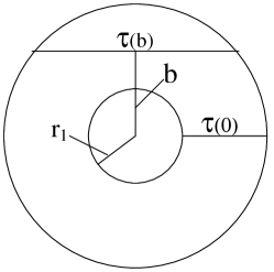
Figure 1: Notation for imaging output.

The surface brightness is a luminosity-independent self-similar distribution [7] of $b/r_{1}$, the impact parameter scaled by the envelope inner radius (fig. 1); note that $r_{1}$ is listed in the default output file (§4.1) for a source luminosity $10^{4}$ $L_{\odot}$. DUSTY can produce maps of the surface brightness at up to 20 wavelengths, specified in the input file. Setting the option flag to 1 produces imaging tabulations for all the models of the run in the single output file fname.itb, setting the flag to 2 puts the table for model number ### in its separate file fname.i###.

Following the option selection flag, the number ($\leq 20$) of desired wavelengths is entered first, followed by a list of these wavelengths in $\mu$m.

• Example of additional input data required in fname.inp for imaging output:

   imaging tables (all models in one file) = 1
   number of wavelengths = 8
   wavelengths = 0.55, 1.0, 2.2, 4, 10, 50, 100, 1000  micron
  

Whenever a specified wavelength is not part of DUSTY’s grid, the corresponding image is obtained by linear interpolation from the neighboring wavelengths in the grid. If the nearest wavelengths are not sufficiently close, the interpolation errors can be substantial. For accurate modeling, all wavelengths specified for imaging should be part of the grid, modifying it if necessary (see §6.2).

Each map is tabulated with a single header line as follows:

• b $=b/r_{1}$, where $b$ is the impact parameter.

• t(b) = $\tau(\tt b)/\tau(0)$, where $\tau(\tt b)$ is the overall optical depth along a path with impact parameter b. Note that $\tau(0)$ is simply the overall radial optical depth tauT, listed in the file fname.s### (§4.2.2), and that t(b) doubles its value across the shell once the impact parameter exceeds the stellar radius.

• The intensity, in Jy arcsec^-2, at each of the wavelengths listed in the header line.

A typical image contains a narrow central spike of width $b_{c}=2r_{c}/r_{1}$, where $r_{c}$ is the radius of the central source [7]. Since this feature is unresolved in most observations, it is usually of limited interest. This spike is the only feature of the emerging intensity that depends on the effective temperature $T_{e}$ of the central source, which is irrelevant to DUSTY’s calculations. The width of the spike scales in proportion to $T_{e}^{-2}$, its height in proportion to $T_{e}^{4}$. The listed value is for $T_{e}=10,000$ K with two exceptions: when the spectral shape of the external radiation is the Planck or Engelke-Marengo function, the arguments of those functions are used for $T_{e}$.

4.2.4 Visibilities

Visibility is the two-dimensional spatial Fourier transform of the surface brightness distribution (for definition and discussion see [7]). Since the surface brightness is a self-similar function of $b/r_{1}$, the visibility is a self-similar function of $q\theta_{1}$ where $q$ is the spatial frequency, $\theta_{1}=2r_{1}/D$ and $D$ is the distance to the source; note that $\theta_{1}$ is listed in the default output file for the location where $F_{\rm obs}=\hbox{$10^{-6}$}\ \rm W\ m^{-2}$ (§4.1).

When imaging tables are produced, DUSTY can calculate from them the corresponding visibility functions. The only required input is the flag triggering this option; if images are not requested in the first place, this entry is skipped. When the visibility option flag is different from zero, it must be the same as the one for imaging. Setting both flags to 1 will add visibility tables for all models to the single file fname.itb. Setting the flags to 2 puts the imaging and visibility tables of each model in the separate file fname.i###, setting them to 3 further splits the output by putting each visibility table in the separate, additional file fname.v###.

Each visibility table starts with a single header line, which lists the specified wavelengths in the order they were entered. The first column lists the dimensionless scaled spatial frequency q = $q\theta_{1}$ and is followed by the visibility tabulation for the various wavelengths.

4.2.5 Radial profiles for each model

The next option flag triggers tabulations of the radial profiles of the density, optical depth and dust temperature. Setting the flag to 1 produces tabulations for all the models of the run in the single output file fname.rtb, setting the flag to 2 places the table for model number ### in its own separate file fname.r###. The tabulated quantities are:

• y – dimensionless radius

• eta – the dimensionless, normalized radial density profile (§3.3)

• t – radial profile of the optical depth variation. At any wavelength $\lambda$, the optical depth at radius $y$ measured from the inner boundary is t*tauT, where tauT is the overall optical depth at that wavelength, tabulated in the file fname.s### (§4.2.2).

• tauF – radial profile of the flux-averaged optical depth

• epsilon – the fraction of grain heating due to the contribution of the envelope to the radiation field (see [9]).

• Td – radial profile of the dust temperature

• rg – radial profile of the ratio of radiation pressure to gravitational force, where both forces are per unit volume:

  $${\hbox{${\cal F}_{\rm rad}$}\over\hbox{${\cal F}_{\rm grav}$}}={3L\over 16\pi GMcr_{gd}}\,{\displaystyle\sum_{i}n_{d,i}a_{i}^{2}\int\!Q_{i,\lambda}f_{\lambda}\,d\lambda\over\displaystyle\sum_{i}n_{d,i}\rho_{s,i}a_{i}^{3}}$$ (7)

  Here $f_{\lambda}=F_{\lambda}/\int F_{\lambda}d\lambda$ is the local spectral shape, $\rho_{s,i}$ is the material solid density and $n_{d,i}$ the number density of grains with size $a_{i}$. The gas-to-dust ratio, $r_{gd}$, appears since the gas is collisionally coupled to the dust. The tabulated value is for $\rho_{s}$ = 3 g cm^-3, $L/M$ = $10^{4}$ $L_{\odot}$/$M_{\odot}$ and $r_{gd}=200$. In the case of radiatively driven winds $r_{gd}$ varies in the envelope because of the dust drift, and this effect is properly accounted in the solution. When the dust optical properties are entered using optical properties = 3, grain sizes are not specified (§3.2.1). This case is handled as described in the last paragraph of §4.1.

In the case of dynamical calculation with density type = 3 for AGB stars (§3.3.2), the following additional profiles are tabulated:

• u – the dimensionless radial velocity profile normalized to the terminal velocity Ve, which is tabulated for the corresponding overall optical depth in file fname.out (§4.1).

• drift – the radial variation of $v_{\rm g}/v_{\rm d}$, the velocity ratio of the gas and dust components of the envelope. This quantity measures the relative decrease in dust opacity due to dust drift.

4.2.6 Detailed Run-time messages

In case of an error, the default output file issues a warning. Optionally, additional, more detailed run-time error messages can be produced and might prove useful in tracing the program’s progress in case of a failure. Setting the corresponding flag to 1 produces messages for all the models in the single output file fname.mtb, setting the flag to 2 puts the messages for model number ### in its own separate file fname.m###.

5 Slab Geometry

DUSTY offers the option of calculating radiative transfer through a plane-parallel dusty slab. The slab is always illuminated from the left, additional illumination from the right is optional.

As long as the surfaces of equal density are parallel to the slab boundaries, the density profile is irrelevant: location in the slab is uniquely specified by the optical depth from the left surface. Unlike the spherical case, there is no reference to spatial variables since the problem can be solved fully in optical-depth space. The other major difference involves the bolometric flux $F$. In the spherical case the diffuse flux vanishes at $y=1$ and $F=F_{e1}/y^{2}$, where $F_{e1}$ is the external bolometric flux at the shell inner boundary [9]. In contrast, $F$ is constant in the slab and the diffuse flux does not vanish on either face. Therefore $F/F_{e1}$, where $F_{e1}$ is the bolometric flux of the left-side source at slab entry, is another unknown variable determined by the solution.

The slab geometry is selected by specifying density type = 0. The dust properties are entered as in the spherical case, with the dust temperature specified on the slab left surface instead of the shell inner boundary. The range of optical depths, too, is chosen as in the spherical case. The only changes from the spherical case involve the external radiation and the output.

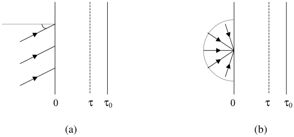
Figure 2: The two possible schemes for a slab illuminated from the left. (a) Parallel rays impinging at an arbitrary angle to the normal. (b) Isotropic radiation.

5.1 Illuminating Source(s)

External radiation is incident from the left side. The presence of an optional right-side source is specified by a non-zero value for R, the ratio of the right-side bolometric flux at slab entry to that of the left-side source. Each input radiation is characterized by its spectral shape, which is entered exactly as in the spherical case (§3.1), and angular distribution. The only angular distributions that do not break the planar symmetry involve parallel rays, falling at some incident angle, and isotropic radiation (see figure 2). The parallel-rays distribution is specified by the cosine ($>0.05$) of the illumination angle, the isotropic distribution is selected by setting this input parameter to $-1$. Since oblique angles effectively increase the slab optical depth, run-times will increase with incidence angle.

• Slab geometry with illumination by parallel rays normal to the left surface. In this case, the spectral shape of the source is entered as in the spherical case. The only change from the spherical input is that the density profile is replaced by the following:

       density type = 0
         cos(angle) = 1.0 (spectral shape entered previously)
                  R = 0   (no source on the right)
  

Two-sided illumination is specified by a non-zero R, where $0<{\tt R}\leq 1$. The properties of the right-side source are specified following the input for R.

• Slab illuminated from both sides. The left-side radiation has isotropic distribution whose spectral shape has been entered previously. The right-side source has a bolometric flux half that of the left-side source and a black-body spectral shape with temperature 3,000 K. It illuminates the slab with parallel rays incident at an angle of $60^{\circ}$ from normal. The density profile is replaced by the following:

     density type = 0
       cos(angle) = -1.0 (spectral shape entered previously)
                R = 0.5
     Properties of the right-side source:
       cos(angle) = 0.5
         Spectrum = 1;   N = 1;  Tbb = 3000 K
  

5.2 Slab Output

The output-control flags are identical to those in the spherical case and the output files are analogous, except for some changes dictated by the different geometry.

5.2.1 Default Output

In the default fname.out. the first two columns are the same as in the spherical case (§4.1) and are followed by:

• Fe1 – bolometric flux, in $\rm W\ m^{-2}$, of the left-side source at the slab left boundary.

• f1 $=F/F_{e1}$, where $F$ is the overall bolometric flux. Values at and below the internal accuracy of DUSTY’s flux computation, $10^{-3}$ when $q_{\rm acc}$ = 0.05, are listed as zero.

• r1(cm) – the distance at which a point source with luminosity $10^{4}$ $L_{\odot}$ produces the bolometric flux $F_{e1}$.

• Td(K) – the dust temperature at the slab right boundary.

• Te(L) – the effective temperature, in K, obtained from $F_{e1}=\sigma{\tt Te}^{4}$. When the slab is illuminated also from the right, a column is added next for Te(R), the effective temperature obtained similarly for the right-side flux.

• err – the flux conservation error, defined as in the spherical case.

5.2.2 Spectral Profiles

Unlike the spherical case, the slab optional spectral files list properties of the half-fluxes emerging from both sides of the slab, calculated over the forward and backward hemispheres perpendicular to the slab faces. The magnitudes of the bolometric half-fluxes on the slab right and left faces can be obtained from tabulated quantities via

$$F_{\rm right}=({\tt R}+{\tt f1})\,{\tt Fe1},\qquad F_{\rm left}=(1-{\tt f1})\,{\tt Fe1}.$$

The right-emerging radiation replaces the spherical output in fname.spp, fname.stb and fname.s###, analogous tables for the left-emerging radiation are simply added to the appropriate output files. Setting the relevant selection flags to 3 places these additional tables in their own separate files — fname.zpp for spectral properties and fname.z### for the detailed spectra of model number ### in the optical depth sequence.

Similar to the fTot column of the spherical case, the spectral shape of the right-emerging half-flux is printed in column fRight. It consists of three components whose fractional contributions are listed next, as in the spherical case: xAtt for the left-source attenuated radiation, xDs and xDe for the diffuse scattered and emitted components, respectively. Subsequent columns are as in the spherical case. The tables for the spectral shape of the left-emerging half-flux fLeft are analogous.

5.2.3 Spatial Profiles

The output for spatial profiles is similar to the spherical case. The radial distance y and density profile eta are removed. The relative distance in optical depth from the left boundary, t, becomes the running variable, and the tabulations of tauF, epsilon and Td are the same (see 4.2.5). The tabulation for ${\cal F}_{\rm rad}$/${\cal F}_{\rm grav}$ is dropped, replaced by three components of the overall bolometric flux: febol is the local net bolometric flux of external radiation; fRbol and fLbol are, respectively, the rightward and leftward half-fluxes of the local diffuse radiation. All components are normalized by Fe1 so that the flux conservation relation is febol + fRbol - fLbol = f1 everywhere in the slab. Note that fRbol vanishes on the slab left face, fLbol on the right face.

DUSTY’s distribution contains two sample input files, slab1.inp and slab2.inp, which can be used as templates for the slab geometry. The output generated with slab1.inp is shown in appendix D.

6 User Control of DUSTY

DUSTY allows the user control of some of its inner working through tinkering with actual code statements that control the spatial and spectral grids. The appropriate statements were placed in the file userpar.inc separate from the main dusty.f, and are imbedded during compilation by the FORTRAN statement INCLUDE. After modifying statements in userpar.inc , DUSTY must be recompiled to enable the changes.

6.1 Array Sizes for Spatial Grid

The maximum size of DUSTY’s spatial grid is bound by array dimensions. These are controlled by the parameter npY which sets the limit on the number of radial points. The default value of 40 must be decreased when DUSTY is run on machines that lack sufficient memory (see §1) and increased when DUSTY fails to achieve the prescribed accuracy (see §3.5). This parameter is defined in userpar.inc via

      PARAMETER (npY=40)

To modify npY simply open userpar.inc, change the number 40 to the desired value, save your change and recompile. That’s all. Every other modification follows a similar procedure. Since DUSTY’s memory requirements vary roughly as the second power of npY, the maximum value that can be accommodated on any given machine is determined by the system memory.

The parameter npY defines also the size npP of the grid used in angular integrations. In the case of planar geometry DUSTY uses analytic expressions for these integrations. Since this grid becomes redundant, npP can be set to unity, allowing a larger maximum npY. The procedure is described in userpar.inc.

6.2 Wavelength Grid

DUSTY’s wavelength grid is used both in the internal calculations and for the output of all wavelength dependent quantities. The number of grid points is set in userpar.inc by the parameter npL, the grid itself is read from the file lambda_grid.dat. This file starts with an arbitrary number of text lines, the beginning of the wavelength list is signaled by an entry for the number of grid points. This number must be equal to npL entered in userpar.inc and to the actual number of entries in the list.

The grid supplied with DUSTY contains 105 points from 0.01 to $3.6\times 10^{4}$ $\mu$m. The short wavelength boundary is to ensure adequate coverage of input radiation from an O star, for example, which peaks at 0.1 $\mu$m. Potential effects on the grain material by such hard radiation are not included in DUSTY. The long wavelength end is to ensure adequate coverage at all wavelengths where dust emission is potentially significant. Wavelengths can be added and removed provided the following rules are obeyed:

1. Wavelengths are specified in $\mu$m.

2. The shortest wavelength must be $\leq 0.01$ $\mu$m, the longest $\geq 3.6\times 10^{4}$ $\mu$m.

3. The ratio of each consecutive pair must be $\leq$ 1.5.

The order of entries is arbitrary, DUSTY sorts them in increasing wavelength and the sorted list is used for all internal calculations and output. This provides a simple, convenient method for increasing the resolution at selected spectral regions: just add points at the end of the supplied grid until the desired resolution is attained. Make sure you update both entries of npL and recompile DUSTY.

In practice, tinkering with the wavelength grid should be reserved for adding spectral features. Specifying the optical properties of the grains at a resolution coarser than that of the wavelength grid defeats the purpose of adding grid points. The optical properties of grains supported by DUSTY are listed on the default wavelength grid. Therefore, modeling of very narrow features requires both the entry of a finer grid in lambda_grid.dat and the input of user-supplied optical properties (see §3.2.1) defined on that same grid.

Appendices

Appendix A Output Summary

DUSTY’s default output is the file fname.out, described in §4.1. Additional output is optionally produced through selection flags, summarized in the following table. The second column lists the section number where a detailed description of the corresponding output is provided.

Table 1: Summary of all Output Options

Output Listing	§	Output File Triggered by Flag
		1	2	3
Spectral properties, all models	4.2.1	fname.spp	fname.spp	fname.spp
Slab, left-face spectra	5.2			fname.zpp
Detailed spectra, each model	4.2.2	fname.stb	fname.s###	fname.s###
Slab, left-face spectra	5.2			fname.z###
Images	4.2.3	fname.itb	fname.i###	fname.i###
Visibilities	4.2.4			fname.v###
Radial profiles	4.2.5	fname.rtb	fname.r###
Error messages	4.2.6	fname.mtb	fname.m###

Appendix B Pitfalls, Real and Imaginary

This appendix provides a central depository of potential programming and numerical problems. Some were already mentioned in the text and are repeated here for completeness.

• FORTRAN requires termination of input records with a carriage return. Make sure you press the “Enter” key whenever you enter a filename in the last line of dusty.inp.

• In preparing input files, the following two rules must be carefully observed: (1) all required input entries must be specified, and in the correct order; (2) the equal sign, ‘=’, must be entered only as a flag to numerical input. When either rule is violated and DUSTY reaches the end of the input file while looking for additional input, you will obtain the error message:

       ****TERMINATED. EOF reached by RDINP while looking for input.
       *** Last line read:
  

  This message is a clear sign that the input is out of order.

• Linux apparently makes heavier demand on machine resources than Windows. On any particular PC and a given value of npY, DUSTY may execute properly under Windows but not under Linux, dictating a smaller npY.

• DUSTY’s execution under the Solaris operating system occasionally gives the following warning message:

         Note: IEEE floating-point exception flags raised:
              Inexact;  Underflow;
          See the Numerical Computation Guide, ieee_flags(3M)
  

  This ominous message is triggered on Solaris also by other applications and is not unique to DUSTY. The reason for it is not yet clear and it is not issued on other platforms. In spite of this statement, the code performs fine and produces results identical to those on machines that do not issue this warning.

• CRAY J90 machines have specific requirements on FORTRAN programs which prevent DUSTY from running in its present form. If you plan to run DUSTY on this platform you’ll have to introduce some changes in the source code, such as replacing all DOUBLE PRECISION statements with REAL*4 .

Appendix C Sample Output File: sphere1.out

 ===========================
  Output from program Dusty
  Version: 2.0
 ===========================

  INPUT parameters from file:
  sphere1.inp

* ----------------------------------------------------------------------
* NOTES:
* This is a simple version of an input file producing a minimal output.
* ----------------------------------------------------------------------
  Central source spectrum described by a black body
  with temperature: 2500 K
  --------------------------------------------
  Abundances for supported grains:
  Sil-Ow Sil-Oc Sil-DL grf-DL amC-Hn SiC-Pg
  1.000  0.000  0.000  0.000  0.000  0.000
  MRN size distribution:
       Power q:  3.5
  Minimal size: 5.00E-03 microns
  Maximal size: 2.50E-01 microns
  --------------------------------------------
  Dust temperature on the inner boundary: 800  K
  --------------------------------------------
  Density described by 1/r**k with k =  2.0
  Relative thickness: 1.000E+03
  --------------------------------------------
  Optical depth at 5.5E-01 microns: 1.00E+00
  Required accuracy: 5%
  --------------------------------------------

  ====================================================
  For compliance with the point-source assumption, the
  following results should only be applied to sources
  whose effective temperature exceeds 1737 K.
  ====================================================

  RESULTS:
  --------
 ###   tau0   F1(W/m2)  r1(cm)    r1/rc   theta1  Td(Y) err
 ###     1        2        3        4        5      6    7
 ==========================================================
   1 1.00E+00 2.88E+04 3.26E+14 8.78E+00 2.43E+00   44   0
 ==========================================================
   (1) Optical depth at 5.5E-01 microns
   (2) Bolometric flux at the inner radius
   (3) Inner radius for L=1E4 Lsun
   (4) Ratio of the inner to the stellar radius
   (5) Angular size (in arcsec) when Fbol=1E-6 W/m2
   (6) Dust temperature at the outer edge (in K)
   (7) Maximum error in flux conservation (%)
 =================================================
  Everything is OK for all models
 ========== THE END ==============================

Appendix D Sample Output File: slab1.out

 ===========================
  Output from program Dusty
  Version: 2.0
 ===========================

  INPUT parameters from file:
  slab1.inp

* ----------------------------------------------------------------------
* NOTES:
* This is a simple version of an input file for calculation in
* planar geometry with single source illumination.
* ----------------------------------------------------------------------
  Left-side source spectrum described by a black body
  with temperature: 2500 K
  --------------------------------------------
  Abundances for supported grains:
  Sil-Ow Sil-Oc Sil-DL grf-DL amC-Hn SiC-Pg
  1.000  0.000  0.000  0.000  0.000  0.000
  MRN size distribution:
       Power q:  3.5
  Minimal size: 5.00E-03 microns
  Maximal size: 2.50E-01 microns
  --------------------------------------------
  Dust temperature on the slab left boundary: 800  K
  --------------------------------------------
  Calculation in planar geometry:
  cos of left illumination angle =   1.000E+00
  R =   0.000E+00
  --------------------------------------------
  Optical depth at 5.5E-01 microns: 1.00E+00
  Required accuracy: 5%
  --------------------------------------------


  RESULTS:
  --------
 ###   tau0    Fe1(W/m2)   f1     r1(cm)  Td(K)  Te(L)  err
 ###     1        2         3       4       5      6     7
 ==========================================================
   1 1.00E+00 2.59E+04  9.33E-01 3.43E+14  755 8.22E+02  0
 ==========================================================
   (1) Optical depth at 5.5E-01 microns
   (2) Bol.flux of the left-side source at the slab left boundary
   (3) f1=F/Fe1, where F is the overall bol.flux in the slab
   (4) Position of the left slab boundary for L=1E4 Lsun
   (5) Dust temperature at the right slab face
   (6) Effective temperature of the left source (in K)
   (7) Maximum error in flux conservation (%)
 =================================================
  Everything is OK for all models
 ========== THE END ==============================

Appendix E Library of Optical Constants

DUSTY’s distribution includes a library of data files with the complex refractive indices of various compounds of interest. The files are standardized in the format DUSTY accepts. Included are the optical constants for the seven built-in dust types as well as other frequently encountered astronomical dust components. This library will be updated continuously at the DUSTY site. The following table lists all the files currently supplied.

Table 2: Optical Constants Library Supplied with Dusty

File Name	Compound	Range ($\mu$m)	Ref
Al2O3-comp.nk	Al2O3-compact	7.8 – 200	[12]
Al2O3-por.nk	Al2O3-porous	7.8 – 500	[12]
amC-hann.nk	amorphous carbon	0.04 – 905	[4]
amC-zb1.nk	amorphous carbon (BE)	0.05 – 1984	[20]
amC-zb2.nk	amorphous carbon (ACAR)	0.04 – 1984	[20]
amC-zb3.nk	amorphous carbon (ACH2)	0.04 – 948	[20]
crbr300.nk	crystalline bronzite	6.7 – 487.4	[5]
crMgFeSil.nk	crystalline silicate	6.7 – 584.9	[12]
FeO.nk	FeO (5.7g/ccm)	0.2 – 500	[12]
gloliMg50.nk	glassy olivine	0.2 – 500	[1]
glpyr300.nk	glassy pyroxene at 300 K	6.7 – 487	[5]
glpyrMg50.nk	glassy pyroxene	0.2 – 500	[1]
glSil.nk	glassy silicate	0.4 – 500	[11]
grph1-dl.nk	graphite, $E\perp c$	0.001 – $10^{3}$	[2]
grph2-dl.nk	graphite, $E\parallel c$	0.001 – $10^{3}$	[2]
opyr-pwd.nk	ortho-pyroxenes - powder	5.0 – 25	[19]
opyr-slb.nk	ortho-pyroxenes - slab	5.0 – 25	[19]
OssOdef.nk	O-deficient CS silicate	0.4 – $10^{4}$	[17]
OssOrich.nk	O-rich IS silicate	0.4 – $10^{4}$	[17]
SiC-peg.nk	$\alpha$-SiC	0.03 – 2000	[18]
Sil-dlee.nk	“Astronomical silicate”	0.03 – 2000	[2]
Sil-oss1.nk	warm O-deficient silicates	0.4 – $10^{4}$	[17]
Sil-oss2.nk	cold O-rich silicate	0.4 – $10^{4}$	[17]

References

- [1] Dorschner, J. et al 1995, A&A 300, 503
- [2] Draine, B.T. & Lee, H.M. 1984, ApJ, 285, 89
- [3] Engelke, C.W. 1992, AJ 104, 1248
- [4] Hanner, M.S. 1988, NASA Conf. Pub. 3004, 22
- [5] Henning, Th. et al 1997, A&A 327, 743
- [6] Ivezić, Ž. & Elitzur, M. 1995, ApJ, 445,415
- [7] Ivezić, Ž. & Elitzur, M. 1996, MNRAS 279, 1011
- [8] Ivezić, Ž. & Elitzur, M. 1996, MNRAS 279, 1019
-
[9]
Ivezić, Ž. & Elitzur, M. 1997, MNRAS 287, 799;
Erratum: MNRAS 303, 864 (1999) - [10] Ivezić, Ž. & Elitzur, M., in preparation
- [11] Jäger, C. et al 1994, A&A 292, 641
-
[12]
Jena–St. Petersburg database of optical constants,
accessible at
http://www.astro.uni-jena.de/Users/database/entry.html, - [13] Jura, M. 1994, ApJ, 434, 713
- [14] Kim S.H., Martin P.G. & Hendry P.D. 1994, ApJ, 422,164
- [15] Marengo M. 1999, in preparation
- [16] Mathis J.S., Rumpl W. & Nordsieck K.H. 1977, ApJ, 217, 425
- [17] Ossenkopf, V., Henning, Th. & Mathis, J.S. 1992, A&A, 261, 567
- [18] Pègouriè, B. 1988, A&A, 194, 335
- [19] Roush, T., et al 1991, Icarus, 94, 191
- [20] Zubko, V.G., et al 1996, MNRAS, 282, 1321