Spatial and Velocity Biases

Abstract

We give a summary of our recent studies of spatial and velocity biases of galaxy-size halos in cosmological models. Recent progress in numerical techniques made it possible to simulate halos in large volumes with a such accuracy that halos survive in dense environments of groups and clusters of galaxies. While the very central parts of clusters still may have been affected by numerical effects, halos in simulations look like real galaxies, and, thus, can be used to study the biases – differences between galaxies and the dark matter. For the standard LCDM model we find that the correlation function and the power spectrum of galaxy-size halos at $z=0$ are antibiased on scales $r<5h^{-1}$Mpc and $k\approx(0.15-30)h$Mpc^-1. The biases depend on scale, redshift, and circular velocities of selected halos. Two processes seem to define the evolution of the spatial bias: (1) statistical bias (or peak bias) and merger bias (merging of galaxies, which happens preferentially in groups, reduces the number of galaxies, but does not affect the clustering of the dark matter). There are two kinds of velocity bias. The pair-wise velocity bias is $b_{12}=0.6-0.8$ at $r<5h^{-1}$Mpc, $z=0$. This bias mostly reflects the spatial bias and provides almost no information on the relative velocities of the galaxies and the dark matter. One-point velocity bias is a better measure of the velocities. Inside clusters the galaxies should move slightly faster ($b_{v}=1.1-1.3$) than the dark matter. Qualitatively this result can be understood using the Jeans equations of the stellar dynamics.

Department of Astronomy, New Mexico State University, Las Cruces, NM 88001

Instituto de Astronomía, Universidad Nacional Autónoma de México, C.P. 04510, México, D.F., México

1. Introduction

The distribution of galaxies is likely biased with respect to the dark matter. Therefore, the galaxies can be used to probe the matter distribution only if we understand the bias. Although the problem of bias has been studied extensively in the past (e.g., Kaiser 1984; Davis et al., 1985; Dekel & Silk 1986), new data on high redshift clustering and the anticipation of coming measurements have recently generated substantial theoretical progress in the field. The breakthrough in analytical treatment of the bias was the paper by Mo & White (1996), who showed how bias can be predicted in the framework of the extended Press-Schechter approximation. More elaborate analytical treatment has been developed by Catelan et al. (1998ab), Porciani et al.(1998), and Sheth & Lemson (1998). Effects of nonlinearity and stochasticity were considered in Dekel & Lahav (1998).

Valuable results are produced by “hybrid” numerical methods in which low-resolution N-body simulations (typical resolution $\sim 20$kpc) are combined with semi-analytical models of galaxy formation (e.g., Diaferio et al., 1998; Benson et al. 1999). Typically, results of these studies are very close to those obtained with brute-force approach of high-resolution ($\sim 2$kpc) N-body simulations (e.g., Colín et al. 1999a). This agreement is quite remarkable because the methods are very different. It may indicate that the biases of galaxy-size objects are controlled by the random nature of clustering and merging of galaxies and by dynamical effects, which cause the merging, because those are the only common effects in those two approaches.

Direct N-body simulations can be used for studies of the biases only if they have very high mass and force resolution. Because of numerous numerical effects, halos in low-resolution simulations do not survive in dense environments of clusters and groups (e.g., Moore, Katz & Lake 1996; Tormen, Diaferio & Syer, 1998; Klypin et al., 1999). Estimates of the needed resolution are given in Klypin et al. (1999). Indeed, recent simulations, which have sufficient resolution have found hundreds of galaxy-size halos moving inside clusters (Ghigna et al., 1998; Colín et al., 1999a; Moore et al., 1999; Okamoto & Habe, 1999).

It is very difficult to make accurate and trustfull predictions of luminosities for galaxies, which should be hosted by dark matter halos. Instead of luminosities or virial masses we suggest to use circular velocities $V_{c}$ for both numerical and observational data. For a real galaxy its luminosity tightly correlate with the the circular velocity. So, one has a good idea what is the circular velocity of the galaxy. Nevertheless, direct measurements of circular velocities of a large complete sample of galaxies are extremely important because it will provide a direct way of comparing theory and observations.

In this paper we give a summary of results presented in Colín et al. (1999ab) and Kravtsov & Klypin (1999).

2. Simulations

We have simulated different cosmological models (Colín et al., 1999a), but our main results are based on currently favored model with the following parameters (s$\Lambda$CDM model): $\Omega_{0}=1-\Omega_{\Lambda}=0.3$, $h=0.7$, $\Omega_{b}=0.032$, $\sigma_{8}=1$. Using the Adaptive Refinement Tree code (ART; Kravtsov, Klypin & Khokhlov, 1997) we run a simulation with $256^{3}$ particles in a 60$h^{-1}$Mpc box. Formal mass and force resolutions are $m_{1}=1.1\times 10^{9}h^{-1}M_{\odot}$ and $2h^{-1}$kpc. Bound Density Maximum halo finder was used to identify halos with at least 30 bound particles. For each halo we find maximum circular velocity $V_{c}=\sqrt{GM(<r)/r}$.

3. Spatial bias

Figure 1 presents a comparison of the theoretical and observational data on correlation functions and power spectra. The dark matter clearly predicts much too high amplitude of clustering. The halos are much closer to the observational points and predict antibias. For the correlation function the antibias appears on scales $r<5h^{-1}$Mpc; for the power spectrum the scales are $k>0.2h{\rm Mpc}^{-1}$. One may get an impression that the antibias starts at longer waves in the power spectrum $\lambda=2\pi/k\approx 30h^{-1}{\rm Mpc}$ as compared with $r\approx 5h^{-1}$Mpc in the correlation function. There is no contradiction: sharp bias at small distances in the correlation function when Fourier transformed to the power spectrum produces antibias at very small wavenumbers. Thus, the bias should be taken into account at long waves when dealing with the power spectra. There is an inflection point in the power spectrum where the nonlinear power spectrum start to go upward (if one moves from low to high $k$) as compared with the prediction of the linear theory. Exact position of this point may have been affected by the finite size of the simulation box $k_{\rm min}=0.105h^{-1}$Mpc, but effect is expected to be small.

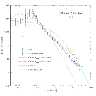
Figure 1.: Correlation function (left) and the power spectrum (right) of halos of different limiting circular velocities in the $\Lambda$CDM model. Results are compared with the observational data from the APM and Stromlo-APM surveys.

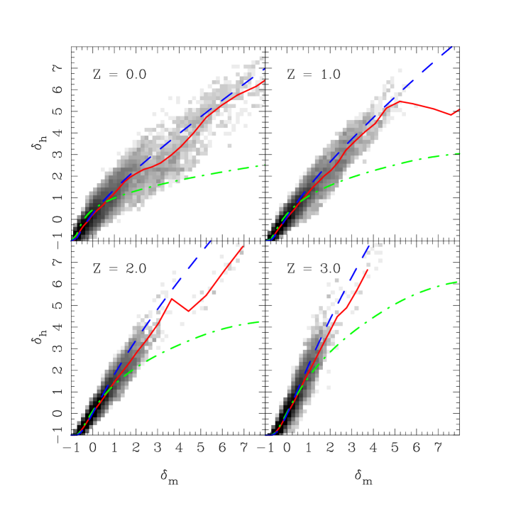
Figure 2.: Overdensity of halos $\delta_{h}$ vs. the overdensity of the dark matter $\delta_{m}$. The overdensities are estimated in spheres of radius $R_{\rm TopHat}=5h^{-1}$Mpc. Intensity of the grey shade corresponds to the natural logarithm of the number of spheres in a 2D grid in $\delta_{h}$- $\delta_{m}$ space. The solid curves show the average relation. The dot-dashed curve is a prediction of an analytical model, which assumes that formation redshift $z_{f}$ of halos coincides with observation redshift (typical assumption for the Press-Schechter approximation). The long-dashed curve is for model, which assumes that substructure survives for some time after it falls into a larger object: $z_{f}=z+1$

At $z=0$ the bias almost does not depend on the mass limit of the halos. There is a tendency of more massive halos to be more clustered at very small distances $r<200h^{-1}$kpc, but at this stage it is not clear that this is not due to residual numerical effects around centers of clusters. The situation is different at high redshift. At very high redshifts $z>3$ galaxy-size halos are very strongly (positively) biased. For example, at $z=5$ the correlation function of halos with $v_{c}>150{\rm km}/{\rm s}$ was 15 times larger than that of the dark matter at $r=0.5h^{-1}$Mpc (see Fig.8 in Colín et al., 1999a). The bias was also very strongly mass-dependent with more massive halos being more clustered. At smaller redshifts the bias was quickly declining. Around $z=1-2$ (exact value depends on halo circular velocity) the bias crossed unity and became less than unity (antibias) at later redshifts.

Evolution of bias is illustrated by Figure 2. The figure shows that at all epochs the overdensity of halos tightly correlates with the overdensity of the dark matter. The slope of the relation depends on the dark matter density and evolves with time. At $z>1$ halos are biased ($\delta_{h}>\delta_{m}$) in overdense regions with $\delta_{m}>1$ and antibiased in underdense regions with $\delta_{m}<-0.5$ At low redshifts there is an antibias at large overdensities and almost no bias at low densities.

4. Velocity bias

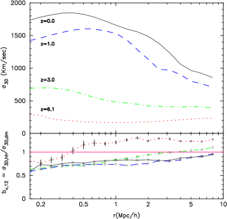
Figure 3.: Left: Evolution with redshift of the pairwise rms velocity of the dark matter (top panel) and the pairwise velocity bias of halos with $V_{c}>90$km/s (bottom panel. Right: Top panel: 3D rms velocity for halos (circles) and for dark matter (full curve) in twelve largest clusters. Bottom panel: velocity bias in the clusters. The bias in the first point increases to 1.2 if the central cD halos are excluded from analysis. Errors correspond to 1-sigma errors of the mean obtained by averaging over 12 clusters at two moments of time. Fluctuations for individual clusters are larger.

There are two statistics, which measure velocity biases – differences in velocities of the galaxies (halos) and the dark matter. For a review of results and references see Colín et al. (1999). Two-particle or pairwise velocity bias (PVB) measures the relative velocity dispersion in pairs of objects with given separation $r$: $b_{12}=\sigma_{\rm halo-halo}(r)/\sigma_{\rm dm-dm}(r)$. It is very sensitive to the number of pairs inside clusters of galaxies, where relative velocities are largest. Removal of few pairs can substantially change the value of the bias. This “removal” happens when halos merge or are destroyed by central cluster halos. One-point velocity bias is estimated as a ratio of the rms velocity of halos to that of the dark matter: $b_{1}=\sigma_{halos}/\sigma_{dm}$. It is typically applied to clusters of galaxies where it is measured at different distances from the cluster center. For our analysis of the velocity bias in clusters we have selected twelve most massive clusters in the simulation. The most massive cluster had virial mass $6.5\times 10^{14}h^{-1}M_{\odot}$ comparable to that of the Coma cluster. The cluster had 246 halos with circular velocities larger than 90 km/s. There were three Virgo-type clusters with virial masses in the range $(1.6-2.4)\times 10^{14}h^{-1}M_{\odot}$ and with approximately 100 halos in each cluster. One cluster was excluded from the analysis because it was in the process of the major merger at $z=0$. Figure 3 shows results for both statistics. Left panels show evolution of the PVB. Just as the spatial bias, PVB is positive at large redshifts (except for the very small scales) and decreases with the redshift. At lower redshifts it does not evolve much and stays below unity (antibias) at scales below $5h^{-1}$Mpc on the level $b_{12}\approx(0.6-0.8)$.

Figure 4.: One-point velocity bias for 3 Virgo-type clusters in the simulation. Central cD halos are not included. Fluctuations in the bias are very large because each cluster has only $\sim$100 halos with $V_{c}>90km/s$ and because of substantial substructure in the clusters.

Right panels show one-point velocity bias in clusters at $z=0$. Note that the sign of the bias is now different: halos move slightly faster than the dark matter. The bias is stronger in the central parts $b_{1}=1.2-1.3$ and goes to almost no bias $b_{1}\approx 1$ at the virial radius and above. Both the antibias in the pairwise velocities and positive one-point bias are produced by the same physical process – merging and destruction of halos in central parts of groups and clusters. The difference is in the different weighting of halos in those two statistics. Smaller number of high-velocity pairs significuntly changes PVB, but it does not affect much the one-point bias because it is normalized to the number of halos at a given distance from the cluster center. At the same time, merging preferentially happens for halos, which move with smaller velocity at a given distance from the cluster center. Slower halos have shorter dynamical times and have smaller apocenters. Thus, they have better chance to be destroyed and merged with the central cD halo. Because low-velocity halos are eaten up by the central cD, velocity dispertion of those, which survive, is larger. Another way of addressing the issue of the velocity bias is to use the Jeans equations. If we have a tracer population, which is in equlibrium in a potential produced by mass $M(<r)$, then

$$-r\sigma_{r}^{2}(r)\left[\frac{d\ln\sigma_{r}^{2}(r)}{d\ln r}+\frac{d\ln\rho(r)}{d\ln r}+2\beta(r)\right]=GM(<r),$$ (1)

where $\rho$ is the number density of the tracer, $\beta$ is the velocity anisotropy, and $\sigma_{r}$ is the rms radial velocity. The r.h.s. of the equation is the same for the dark matter and the halos. If the term in the brackets would be the same, there would be no velocity bias. But there is systematical difference between the halos and the dark matter: the slope of the distribution halos in a cluster $\frac{d\ln\rho(r)}{d\ln r}$ is smaller than that of the dark matter (see Colín et al., 1998, Ghigna et al., 1999). The reason for the difference of the slopes is the same – merging with the central cD. Other terms in the equation also have small differences, but the main contribution comes from the slope of the density. Thus, as long as we have spatial antibias of the halos, there should be a small positive one-point velocity bias in clusters and a very strong antibias in pairwise velocity. Exact values of the biases are still under debate, but one thing seems to be certain: one bias does not go without the other.

The velocity bias in clusters is difficult to measure because it is small. The right panel in Figure 3 may be misleading because it shows the average trend, but it does not give the level of fluctuations for a single cluster. Note that the errors in the plots correspond to the error of the mean obtained by averaging over 12 clusters and two close moments of time. Fluctuations for a single cluster are much larger. Figure 3 shows results for three Virgo-type clusters in the simulation. The noice is very large because of both poor statistics (small number of halos) and the noise produced by residual non-equilibrium effects (substructure). Comparable (but slightly smaller) value of $b_{v}$ was recently found in simulations by Ghigna et al. (1999, astro-ph/9910166) for a cluster in the same mass range as in Figure 3. Unfortunately, it is difficult to make detailed comparison with their results because Ghigna et al. (1999) use only one hand-picked cluster for a different cosmological model. Very likely their results are dominated by the noise due to residual substructure. Results of another high-resolution simulation by Okamoto & Habe (1999) are consistant with our results.

5. Conclusions

There is a number of physical processes, which can contribute to the biases. In our papers we explore dynamical effects in the dark matter itself, which result in differences of the spatial and velocity distribution of the halos and the dark matter. Other effects related to the formation of luminous parts of galaxies also can produce or change biases. At this stage it is not clear how strong are those biases. Because there is a tight correlation between the luminosity and circular velocity of galaxies, any additional biases are limited by the fact that galaxies “know” how much dark matter they have.

Biases in the halos are reasonably well understood and can be approximated on a few Megaparsec scales by analytical models. We find that the biases in the distribution of the halos are sufficient to explain within the framework of standard cosmological models the clustering properties of galaxies on a vast ranges of scales from 100 kpc to dozens Megaparsecs. Thus, there is neither need nor much room for additional biases in the standard cosmological model.

In any case, biases in the halos should be treated as benchmarks for more complicated models, which include non-gravitational physics. If a model can not reproduce biases of halos or it does not have enough halos, it should be rejected, because it fails to have correct dynamics of the main component of the Universe – the dark matter.

References

Benson, A.J., Cole, S., Frenk, C.S., Baugh, C.M., & Lacey, C.D. 1999, MNRAS, submitted (astro-ph/9903343)

Catelan, P., Matarrese, S.,& Porciani, C. 1998a, ApJ, 502, 1

Catelan, P., Lucchin, F., Matarrese, S., & Porciani, C. 1998b, MNRAS, 297, 692

Colín, P., Klypin, A.A., Kravtsov, A.V., & A.M. Khokhlov. 1999a, ApJ, 523, 32 (astro-ph/9809202)

Colín, P., Klypin, A., Kravtsov, A. 1999b, ApJ, submitted (astro-ph/9907337)

Davis, M., Efstathiou, G., Frenk, C.S., & White, S.D.M. 1985, ApJ, 292, 371

Dekel,A., & Silk, J. 1986, ApJ, 303, 39

Dekel, A., & Lahav, O. 1998, ApJ, submitted (astro-ph/9806193)

Diaferio, A., Kauffmann, G., Colberg, J.M., & White, S.D.M.., 1998, MNRAS, submitted (astro-ph/9812009)

Ghigna, S., Moore, B., Governato, F., Lake, G., Quinn, T., Stadel, J. 1998, MNRAS, 300, 146

Gnigna, S., Moore, B., Governato, F., Lake, G., Quinn, T., Stadel, J. 1999, astro-ph/9910166

Kaiser, N. 1984, ApJ, 284, L9

Klypin, A., Gotlöber, S., A.V. Kravtsov, Khokhlov, A. 1999, ApJ, 516, 530

Kravtsov, A.V., & Klypin, A. 1999, ApJ, 520, 437 (astro-ph/9812311)

Kravtsov, A.V., Klypin, A., & Khokhlov, A.M. 1997, ApJS 111, 73

Mo, H.J., & White, S.D.M. 1996, MNRAS, 282, 347

Moore, B., Katz, N., & Lake, G. 1996, ApJ, 456, 455

Moore et al., 1999, ApJ, submitted (astro-ph/9907411)

Okamoto, T., & Habe, A. 1999, ApJ, 516, 591

Porciani, C., Matarrese, S., Lucchin, F., & Catelan, P. 1998, MNRAS, 298, 1097 (astro-ph/9801290)

Sheth, R.K., & Lemson, G. 1999, MNRAS, 305, 946 (astro-ph/9808138)

Tormen, G., Diaferio, A., & Syer, D., 1998, MNRAS, 299, 728.