Comparing the SBF Survey Velocity Field with the Gravity Field from Redshift Surveys

Abstract

We compare the predicted local peculiar velocity field from the IRAS 1.2 Jy flux-limited redshift survey and the Optical Redshift Survey (ORS) to the measured peculiar velocities from the recently completed SBF Survey of Galaxy Distances. The analysis produces a value of $\beta{\,=\,}\Omega^{0.6}/b$ for the redshift surveys, where $b$ is the linear biasing factor, and a tie to the Hubble flow, i.e., a value of $H_{0}$, for the SBF Survey. There is covariance between these parameters, but we find good fits with $H_{0}\approx 74$ km s${}^{-1}\,$Mpc for the SBF distances, $\beta_{I}\approx 0.44$ for the IRAS survey predictions, and $\beta_{O}\approx 0.3$ for the ORS. The small-scale velocity error $\sigma_{v}\sim 200$ km s^-1 is similar to, though slightly larger than, the value obtained in our parametric flow modeling with SBF.

Palomar Observatory, Caltech, MS 105-24, Pasadena, CA 91125

Dept. of Astronomy, University of California, Berkeley, CA 94720

Institute for Astronomy, University of Hawaii, Honolulu, HI 96822

Kitt Peak National Observatory, P. O. Box 26732, Tucson, AZ 85726

Carnegie Observatories, 813 Santa Barbara St., Pasadena, CA 91101

1. The SBF Survey

The Surface Brightness Fluctuation (SBF) method of estimating early-type galaxy distances has been around for over a decade (Tonry & Schneider 1988). Blakeslee, Ajhar, & Tonry (1999) have recently reviewed the SBF method, its applications, and calibration. Tonry, Ajhar, & Luppino (1990) made the first application in the Virgo cluster and calibrated it using theoretical isochrones for the color dependence combined with the Cepheid distance to M31 for the zero point. Tonry (1991) applied the method to Fornax galaxies and made the first fully empirical calibration, differing substantially from the earlier theoretical one. The situation is now much improved, with the best theoretical models (Worthey 1994) agreeing well with the latest empirical calibration.

The $I$-band SBF Survey of Galaxy distances began in earnest in the early 1990’s using the 2.4 m telescope at MDM Observatory on Kitt Peak in the Northern hemisphere and the 2.5 m at Las Campanas Observatory in the South. The Survey includes distances to over 330 galaxies reaching out to $c{z}\sim 4500$ km s^-1. Tonry et al. (1997; hereafter SBF-I) describe the SBF Survey sample in detail. The breakdown by morphology is 55% ellipticals, 40% lenticulars, and 5% spirals. The median distance error is about 0.2 mag, several times larger than our estimate of the intrinsic scatter in the method. This is due to the compromises involved in conducting a large survey with an observationally demanding method on small telescopes; thus, most individual galaxy distances could be improved with reobservation in more favorable conditions.

Tonry et al. (1999, hereafter SBF-II) investigate the large-scale flow field within and around the Local Supercluster using extensive parametric modeling. This modeling is summarized by Tonry et al. and Dressler et al. in the present volume. Also in this volume are SBF-related works by Pahre et al. calibrating the $K$-band fundamental plane with SBF Survey distances and by Liu et al. reporting $K$-band SBF measurements in the Fornax and Coma clusters. Here we present a preliminary comparison of the SBF survey peculiar velocities with expectations from the density field as probed by redshift surveys. More details on many aspects of this work are given by Blakeslee et al. (2000).

2. Comparing to the Density Field

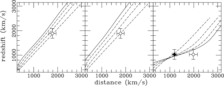
Figure 1.: Predicted $c{z}$–$d$ relations for some individual galaxies. The points are placed according to their observed velocity and SBF distance; the curves are predictions for $\beta=0.1,0.4,0.7,1.0$, with $\beta{\,=\,}1$ being the solid curve. The overall distance scale (i.e., $H_{0}$) is a free parameter; thus for each $\beta$, the $\chi^{2}$ analysis allows the data points to slide uniformly in the horizontal direction. The left and center panels exhibit the same galaxy (NGC 821) with $c{z}$–$d$ curves from the IRAS survey (left) and the ORS (center). The ORS curves fan out more at high $\beta$. They also “bend” more in the presence of mass concentrations, but the right panel shows that even the $\beta{\,=\,}1$ ORS predictions from the spherical harmonic method cannot accommodate a galaxy behind Virgo with a large infall velocity (open point), i.e., they cannot reproduce multivalued zones. Note that a galaxy near the center of Virgo (solid point) helps little in distinguishing between the $\beta$ curves, which cross at this point.

We use the method of Nusser & Davis (1994; see the description by Davis in this volume) to perform a spherical harmonic solution of the gravity field from the observed galaxy distribution of both the IRAS 1.2 Jy flux-limited redshift survey (Strauss et al. 1992; Fisher et al. 1995) and the Optical Redshift Survey (ORS) (Santiago et al. 1995). We assume linear biasing so that the fluctuations in the galaxy number density field are proportional to the mass density fluctuations, i.e., $\delta_{g}=b\,\delta_{m}$, where $b$ is the bias factor, and use linear gravitational instability theory (e.g., Peebles 1993) so that the predicted peculiar velocities are determined by $\beta{\,\equiv\,}\Omega^{0.6}/b$. We then compute the distance-redshift relation in the direction of each sample galaxy as a function of $\beta$.

The comparisons are done with the same subset of SBF survey galaxies as used in SBF-II: galaxies with good quality data, $(V{-}I)_{0}>0.9$ so that the color calibration applies, and not extreme in their peculiar velocities (e.g., no Cen-45); we also omit Local Group members. The sample is then 280 galaxies. We compare the predicted $c{z}$–$d$ relations to the observations using a simple $\chi^{2}$ minimization approach, as adopted by Riess et al. (1997) in the comparison to the Type Ia supernova (SNIa) distances. Figure 1 gives an illustration. Unlike SNIa distances however, the SBF distances have no secure external tie to the far-field Hubble flow, so we allow the overall scale of the distances (in km/s) to be a free parameter. The best-fit scale then yields a value for $H_{0}$ when combined with the SBF tie to the Cepheids, which is uncertain at the $\pm 0.1$ mag level (SBF-II). Thus, the 15 or more free parameters of SBF-II are here replaced by just two parameters: $H_{0}$ and $\beta$.

Our sample consists mainly of early-type galaxies in groups, with the dominant groups being the Virgo and Fornax clusters. We use a constant small-scale velocity error $\sigma_{v}=200$ km s^-1 and deal with group/cluster virial dispersions by using group-averaged redshifts for the galaxies. The group definitions are from SBF-I; more than a third of the galaxies are not grouped. This approach is unlike that of SBF-II, which used only individual galaxy velocities but a variable $\sigma_{v}$. Blakeslee et al. (2000) explore several approaches in doing the comparison to the gravity field, including one with no grouping but a variable $\sigma_{v}$, and find similar results to what we report below. In addition, they find negligibly different results when $\sigma_{v}=150$ km s^-1 is used instead of 200 km s^-1.

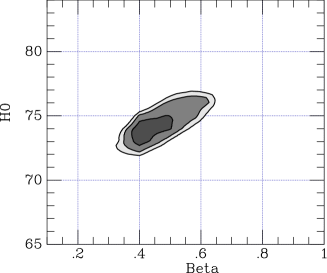
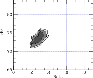
Figure 2.: The 68%, 90%, and 95% joint probability contours on $H_{0}$ and $\beta$ for the comparison between the SBF peculiar velocities and the predictions from the IRAS 1.2 Jy redshift survey (left) and the ORS (right). The irregular, ragged contours are due to the coarseness of the grids.

3. Results

Figure 2 displays the joint probability contours on $H_{0}$ and $\beta$ derived from the $\chi^{2}$ analysis of the IRAS/SBF and ORS/SBF comparisons. The calculations are done in $\beta$ steps of 0.1 and $H_{0}$ steps of 1 km s${}^{-1}\,$Mpc. Both redshift surveys call for $H_{0}\approx 74$ km s${}^{-1}\,$Mpc. For $\beta$, the IRAS comparison gives $\beta_{I}=0.4$–0.5, while the ORS prefers $\beta_{O}\approx 0.3$. Adopting the best $\beta$ models for each comparison, Figure 3 shows the reduced $\chi^{2}$ for 279 degrees of freedom plotted against $H_{0}$ (we averaged the $\beta_{I}=0.4$ and $\beta_{I}=0.5$ predictions for IRAS). As there can only be one $H_{0}$, and the IRAS and ORS surveys are not wholly independent, it is perhaps not surprising that they give consistent results. Interestingly, the preferred $H_{0}$ splits the difference between the “SBF $H_{0}$” values proffered by SBF-II and Ferrarese et al. (1999).

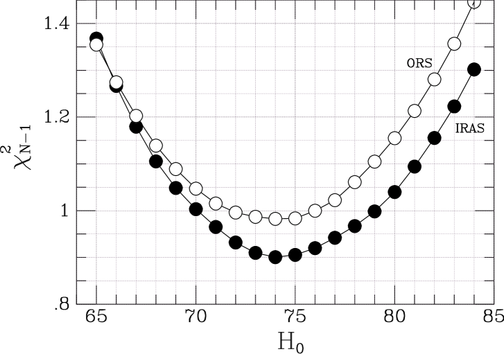
Figure 3.: Reduced $\chi^{2}$ as a function of $H_{0}$ for $\beta_{I}=0.45$ and $\beta_{O}=0.30$. The minimum is reached near $H_{0}=74$ or 74.5 km s${}^{-1}\,$Mpc.

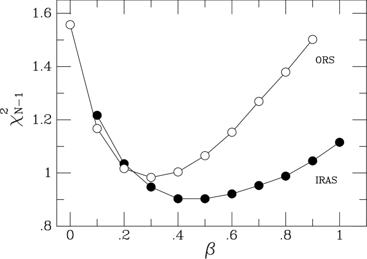
Figure 4.: Reduced $\chi^{2}$ as a function of $\beta$ for $H_{0}=74.5$ km s${}^{-1}\,$Mpc.

The reduced $\chi^{2}$ as a function of $\beta$ for a fixed $H_{0}$ is shown in Figure 4. We find $\beta_{I}=0.44\pm 0.08$ for IRAS and $\beta_{O}=0.30\pm 0.06$ for the ORS with the adopted $H_{0}$. We see that $\sigma_{v}=200$ km s^-1 gives $\chi^{2}_{\nu}{\,=\,}1$ for the ORS comparison, and 0.9 for the IRAS comparison; the latter would have $\chi^{2}_{\nu}{\,=\,}1$ for $\sigma_{v}=180$ km s^-1, very similar to the value of $\sigma_{v}$ found in the SBF-II parametric modeling. The derived $\beta$’s are not sensitive to the adopted $\sigma_{v}$, but they are to $H_{0}$ because of the covariance seen in Figure 2. Had we adopted an $H_{0}$ 5% larger, the best-fit $\beta$’s would increase by $\sim\,$30% with still reasonable values of $\chi^{2}$.

Figure 5.: The residuals (observed minus predicted peculiar velocity) for the IRAS 1.2 Jy survey/SBF Survey comparison with the best-fitting combination of $H_{0}$ and $\beta_{I}$. The three most distant points exhibit small scatter because they are high quality HST measurements.

We also note that the $\beta$’s are insensitive to our treatment of the clusters. We experimented by throwing out all galaxies conceivably near the triple-valued zones of Virgo, Fornax, and Ursa Major, 40% of the sample. Remarkably, the results differ only negligibly, but $\chi^{2}_{\nu}$ increases by about 0.15, and the values of $\sigma_{v}$ giving $\chi^{2}_{\nu}$ of unity increase by 10%. The IRAS residual plot for the full comparison shown in Figure 5 demonstrates why. The Virgo and Fornax clusters near $c{z}$ of 1000 and 1400 km s^-1, respectively, lie close to the zero-difference line with fairly small scatter because they have had their virial dispersions effectively removed, unlike most of the rest of the galaxies. However, for the reason illustrated in Figure 1, the clusters do not drive the fit.

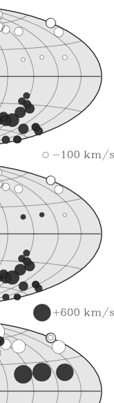
Figure 6.: Predicted peculiar velocities from the ORS for $\beta_{O}=0.3$ (top) and IRAS for $\beta_{I}=0.4$ (middle) are compared to observed peculiar velocities from the SBF Survey (bottom) with $H_{0}=74$ km s${}^{-1}\,$Mpc. Velocities are in the Local Group frame and coordinates are Galactic. Light/dark circles show negative/positive peculiar velocities, coded in size as shown. Unlike the predictions, the observations have no smoothing applied and contain both distance and velocity errors, causing the greater range in symbol size.

Figure 6 shows how the peculiar velocity predictions and observations look on the sky. The predictions should resemble a noiseless, smoothed version of the observations. Clearly there is general agreement on the most prominent feature, the dipole motion seen in the Local Group frame. The observed large negative velocities near $(l,b)\sim(283^{\circ},+74^{\circ})$ indicate rapidly infalling Virgo background galaxies, which as noted in Figure 1, the fit cannot reproduce. This and other issues must be dealt with in future analyses.

4. Summary and Future Prospects

We have presented preliminary results from an initial comparison of the SBF Survey peculiar velocities with predictions based on the density field of the IRAS and ORS redshift surveys. The comparison simultaneously yields $\beta$ for the density field and a tie to the Hubble flow for SBF, i.e., $H_{0}$. The resulting $H_{0}\approx 74$ is between the two other recent estimates with SBF. For the IRAS comparison we find $\beta_{I}\approx 0.44$, consistent with other recent results populating the 0.4–0.6 range from “velocity-velocity” comparisons using Tully-Fisher or SNIa distances (e.g., Schlegel 1995; Davis et al. 1996; Willick et al. 1997; Riess et al. 1997; da Costa et al. 1998; Willick & Strauss 1998). Our value of $\beta_{O}\approx 0.30$ is the same as that of Riess et al., and consistent with the expectation $\beta_{O}/\beta_{I}\sim 0.7$ from Baker et al. (1998). The numbers change only slightly with different treatments of the galaxy clusters and higher resolution computations (Blakeslee et al. 2000). Our results thus reinforce the “factor-of-two discrepancy” with the high $\beta$’s obtained in “density-density” comparisons (e.g., Sigad et al. 1998). One explanation is a scale-dependent biasing (e.g., Dekel, this volume).

We plan in the near future to pursue comparisons using methods that can deal with multivalued redshift zones directly, such VELMOD (Willick et al. 1997) and take advantage of SBF’s potential for probing small, nonlinear scales. Additionally, we continue to work towards an independent far-field tie to the Hubble flow by measuring SBF distances to SNIa galaxies, through calibration of the $K$-band fundamental plane Hubble diagram (Pahre et al., this volume), and by pushing out to $c{z}\sim 10,000$ km s^-1 directly using SBF measurements from space. This will remove the substantial systematic uncertainty in $\beta$ due to the covariance with $H_{0}$. Finally, we also plan to use SBF data for a “density-density” measurement of $\beta$ and to explore the nature of the biasing.

Acknowledgments.

JPB thanks the Sherman Fairchild Foundation for support. The SBF Survey was supported by NSF grant AST9401519.

References

Baker, J. E., Davis, M., Strauss, M. A., Lahav, O., Santiago, B. X. 1998, ApJ, 508, 6

Blakeslee, J. P., Ajhar, E. A., & Tonry, J. L. 1999, in Post-Hipparcos Cosmic Candles, eds. A. Heck & F. Caputo (Boston: Kluwer Academic), 181

Blakeslee, J. P., Davis, M., Tonry, J. L., Dressler, A., & Ajhar, E. A. 2000, ApJ, in press

da Costa, L. N., Nusser, A., Freudling, W., Giovanelli, R., Haynes, M. P., Salzer, J. J., & Wegner, G. 1998, MNRAS, 299, 425

Davis, M., Nusser, A. & Willick, J. A. 1996, ApJ, 473, 22

Ferrarese, L., et al. ($H_{0}$ Key Project) 1999, ApJ, in press

Fisher, K. B., Huchra, J. P., Strauss, M. A., Davis, M., Yahil, A., & Schlegel, D. 1995, ApJS, 100, 69

Nusser, A. & Davis, M. 1994, ApJ, 421, L1

Peebles, P.J.E. 1993, Principles of Physical Cosmology (Princeton Univ. Press)

Riess, A. G., Davis, M., Baker, J., & Kirshner, R. P. 1997, ApJ, 488, L1

Santiago, B. X., Strauss, M. A., Lahav, O., Davis, M., Dressler, A., & Huchra, J. P. 1995, ApJ, 446, 457

Schlegel, D. J. 1995, Ph.D. Thesis, Univ. of California, Berkeley

Sigad, Y., Eldar, A., Dekel, A., Strauss, M. A., & Yahil, A. 1998, ApJ, 495, 516

Strauss, M. A., Huchra, J. P., Davis, M., Yahil, A., Fisher, K. B., & Tonry, J. 1992, ApJS, 83, 29

Tonry, J. L. 1991, ApJ, 373, L1.

Tonry, J. L., Ajhar, E. A., & Luppino, G. A. 1990, AJ, 100, 1416

Tonry, J. L., Blakeslee, J. P., Ajhar, E. A., & Dressler, A. 1997, ApJ, 475, 399 (SBF-I)

Tonry, J. L., Blakeslee, J. P., Ajhar, E. A., & Dressler, A. 1999, ApJ, in press (SBF-II)

Tonry, J. L. & Schneider, D. P. 1988, AJ, 96, 807

Willick, J. A., Strauss, M. A., Dekel, A., & Kolatt, T. 1997, ApJ, 486, 629

Willick, J. A. & Strauss, M. A. 1998, ApJ, 507, 64