A First Comparison of the SBF Survey Distances with the Galaxy Density Field: Implications for $H_{0}$ and $\Omega$

Abstract

We compare the peculiar velocities measured in the SBF Survey of Galaxy Distances with the predictions from the density fields of the IRAS 1.2 Jy flux-limited redshift survey and the Optical Redshift Survey (ORS) to derive simultaneous constraints on the Hubble constant $H_{0}$ and the density parameter $\beta=\Omega^{0.6}/b$, where $b$ is the linear bias. We find $\beta_{I}=0.42^{+0.10}_{-0.06}$ and $\beta_{O}=0.26\pm 0.08$ for the IRAS and ORS comparisons, respectively, and $H_{0}=74\pm 4$ km s${}^{-1}\,$Mpc (with an additional 9% uncertainty due to the Cepheids themselves). The match between predicted and observed peculiar velocities is good for these values of $H_{0}$ and $\beta$, and although there is covariance between the two parameters, our results clearly point toward low-density cosmologies. Thus, the unresolved discrepancy between the “velocity-velocity” and “density-density” measurements of $\beta$ continues.

1. Introduction

Gravitational instability theory posits that the present-day peculiar velocity $v_{p}$ of a galaxy will equal the time-integral of the gravitational acceleration due to nearby mass concentrations, i.e., $v_{p}=\langle g\rangle t$. For galaxies outside virialized structures, linear perturbation theory can be used to relate $v_{p}$ to the present-day local mass density:

$$v_{p}(\mbox{\boldmath$r$})\approx\frac{\Omega^{0.6}H_{0}}{4\pi}\int{d^{3}\mbox{\boldmath$r^{\prime}$}\delta_{m}(\mbox{\boldmath$r^{\prime}$})\frac{\mbox{\boldmath$r^{\prime}-r$}}{|\mbox{\boldmath$r^{\prime}-r$}|^{3}}}$$ (1)

(Peebles 1980), where $\Omega$ is the mass density of the universe in units of the critical density, $H_{0}$ is the Hubble constant, and $\delta_{m}(r)$ is the mass density fluctuation field. A further common simplification is the linear biasing model, $\delta_{g}=b\,\delta_{m}$, where $\delta_{g}$ is the fluctuation field of the observed galaxy distribution, and $b$ is the linear bias. With these assumptions, the observed peculiar velocity will be proportional to the quantity $\beta=\Omega^{0.6}/b$.

Redshift surveys of complete samples of galaxies can be used to determine the galaxy density in redshift space $\delta_{g}(z)$, which is then smoothed and used to predict the peculiar velocity field. In this case, the distances are measured in units of the Hubble velocity and $H_{0}$ cancels out of Eq. (1). Comparison with observed peculiar velocities from distance surveys tied to the Hubble flow then yields a value for $\beta$ (see Strauss & Willick [1995] for a comprehensive review of the methods). Recent applications using Tully-Fisher distances and the density field of the IRAS 1.2 Jy redshift survey (Fisher et al. 1995) have found best-fit values $\beta_{I}=0.4$–0.6 (Schlegel 1995; Davis et al. 1996; da Costa et al. 1998; Willick et al. 1997; Willick & Strauss 1998), where the subscript denotes the IRAS survey. Riess et al. (1997) have done the comparison with Type Ia supernovae (SNIa) distances and find $\beta_{I}=0.40\pm 0.15$. On the other hand, the Potent method (Dekel et al. 1990), based on the derivative of Eq. (1) but incorporating nonlinear terms, gives a $\beta_{I}$ about twice this value, most recently $\beta_{I}=0.89\pm 0.12$ (Sigad et al. 1998).

The surface brightness fluctuation (SBF) method (Tonry & Schneider 1988) of measuring early-type galaxy distances is new to the field of cosmic flows. A full review of the method is given by Blakeslee et al. (1999). The $I$-band SBF Survey (Tonry et al. 1997, hereafter SBF-I) gives distances to about 300 galaxies out to $\sim\,$4000 km s^-1. Tonry et al. (1999, hereafter SBF-II) used these data to construct a parametric flow model of the surveyed volume, but as the analysis made no use of galaxy distribution information, it could not constrain $\Omega$. It did, however, allow for a direct tie between the Cepheid-calibrated SBF distances and the unperturbed Hubble flow, and thus a value for $H_{0}$. Previous $H_{0}$ estimates with SBF (e.g., Tonry 1991; SBF-I) relied on far-field ties to methods such as Tully-Fisher, $D_{n}$–$\sigma$, and SNIa, and thus incurred additional systematic uncertainty. Unfortunately, this “direct tie” of SBF to the Hubble flow was still not unambiguous. For instance, Ferrarese et al. (1999, hereafter F99) used a subset of the same SBF data but a different parametric flow model to derive an $H_{0}$ 10% lower than in SBF-II.

The present work uses SBF Survey distances in an initial comparison to the peculiar velocity predictions from redshift surveys and derives simultaneous constraints on $H_{0}$ and $\beta$. The comparison also provides tests of linear biasing, the SBF distances, and claimed bulk flows.

2. Analysis

We compute the redshift-distance ($c{z}$–$d$) relation in the direction of each sample galaxy using the method of Davis & Nusser (1994), which performs a spherical harmonic solution of the redshift-space version of the Poisson equation. Computations are done for both the IRAS 1.2 Jy (Fisher et al.1995) and “Optical Redshift Survey” (Santiago et al. 1995) catalogs as a function of their respective density parameters $\beta_{I}$ and $\beta_{O}$. The smoothing scale of the $c{z}$–$d$ predictions is typically $\sim\,$500 km s^-1.

The predictions are then compared to the SBF observations using the $\chi^{2}$ minimization approach adopted by Riess et al. (1997), who assumed a fixed “redshift error” of $\sigma_{v}{\,=\,}200$ km s^-1. This term includes uncertainty in the linear predictions, unmodeled nonlinear motions, and true velocity measurement error; we also report results with $\sigma_{v}{\,=\,}150$ km s^-1. We use the same subset of galaxies as in SBF-II, namely those with high-quality data, $(V{-}I)_{0}>0.9$, and not extremely anomalous in their velocities (e.g., Cen-45); we also omit Local Group members. The full sample then comprises 280 galaxies. Unlike the case for the SNIa distances, we lack a secure external tie to the Hubble flow, so we successively rescale the SBF distances to different values of $H_{0}$ and repeat the minimization.

The Nusser-Davis method cannot reproduce the multivalued $c{z}$–$d$ zones of clusters, but it can produce major stall regions in the $c{z}$–$d$ relation. Since such regions will have high velocity dispersions, this deficiency in the method may be overcome with allowance for extra velocity error. A significant fraction of SBF galaxies reside in the Virgo and Fornax clusters. We adopt the following three approaches in dealing with these. “Trial 1” uses individual galaxy velocities but allows extra variance in quadrature for the clusters according to: $\sigma_{\rm cl}(r)=\sigma_{0}/\sqrt{1+(r/r_{0})^{2}}$, where $\sigma_{0}=700\,(400)$ km s^-1 and $r_{0}=2\,(1)$ Mpc are adopted for Virgo (Fornax). These spatial profiles are meant to mimic the observed projected profiles and parameters from Fadda et al. (1996) and Girardi et al. (1998); at large-radius $\sigma_{\rm cl}$ follows the infall velocity profile (e.g., SBF-II). “Trial 2” uses a fixed velocity error but removes the virial dispersions by assigning galaxies their group-averaged velocities. The groups are defined in SBF-I: 29 galaxies are grouped into Virgo, 27 into Fornax, 7 into Ursa Major, and all other groups have 2-6 members, with 34% of the sample being ungrouped. “Trial 3” is similar to trial 2, but 72 sample galaxies within 10 Mpc of Virgo (about 50% larger than the zero-velocity radius found in SBF-II) and 30 within 5 Mpc of Fornax are removed, reducing the sample by 36% to 178 galaxies.

For each of the trials, we calculate $\chi^{2}$ for the comparisons with both the IRAS and ORS gravity fields, using $\sigma_{v}$ of both 150 and 200 km s^-1, for a range in $H_{0}$ in steps of 0.1 km s${}^{-1}\,$Mpc and a range in $\beta$ in steps of 0.1. We then interpolate in $\beta$ by cubic splines to find the $H_{0}$-$\beta$ combination minimizing $\chi^{2}$.

3. Results

Figure 3 shows the 68%, 90%, and 99% joint confidence contours on $H_{0}$ and $\beta$ from the $\chi^{2}$ analyses for trial 2 (which gives the median best-fit $H_{0}$) using $\sigma_{v}=200$ km s^-1. Significant covariance exists between the two parameters. Table 1 shows the $\chi^{2}$ minimization results for all the different comparison runs. In order to give a more realistic impression of the true uncertainties, the tabulated errors are for $\delta\chi^{2}=2.3$, the 68% joint confidence range on 2 parameters, except for the last column which varies $H_{0}$ within uncertainty limits to explicitly take account of the covariance in $\beta$ (see below).

Figure 1.— The 68%, 90%, and 99% joint probability contours on $H_{0}$ and $\beta{\,\equiv\,}\Omega^{0.6}/b$ are plotted for the “Trial 2” comparison (see §2 for description) of the SBF peculiar velocities against the IRAS (solid curves at right) and ORS (dotted curves at left) density field predictions. Crosses mark the best-fit positions.

Table 1Results from Peculiar Velocity Comparisons

Run	$\sigma_{v}$	$\chi^{2}_{\nu}$	$\beta$  $\pm$	$H_{0}$$\pm$	$\beta_{H_{0}{=}74}\,\pm$
IRAS–1	200	0.99	0.39  0.06	73.2  1.2	0.42  ${}^{+0.10}_{-0.07}$
IRAS–1	150	1.21	0.40  0.07	73.7  1.1	0.41  ${}^{+0.09}_{-0.06}$
IRAS–2	200	0.89	0.43  0.06	73.9  1.0	0.43  ${}^{+0.10}_{-0.06}$
IRAS–2	150	1.18	0.45  0.06	74.3  1.0	0.44  ${}^{+0.08}_{-0.05}$
IRAS–3	200	1.05	0.40  0.08	74.1  1.2	0.40  ${}^{+0.10}_{-0.05}$
IRAS–3	150	1.33	0.41  0.07	74.4  1.2	0.41  ${}^{+0.07}_{-0.05}$
ORS–1	200	1.05	0.23  0.05	72.1  1.2	0.25  ${}^{+0.07}_{-0.05}$
ORS–1	150	1.28	0.24  0.05	72.4  1.0	0.27  ${}^{+0.06}_{-0.05}$
ORS–2	200	0.97	0.25  0.05	72.8  1.3	0.29  ${}^{+0.06}_{-0.07}$
ORS–2	150	1.29	0.27  0.05	73.1  1.2	0.30  ${}^{+0.05}_{-0.05}$
ORS–3	200	1.12	0.22  0.05	74.1  1.4	0.21  ${}^{+0.05}_{-0.04}$
ORS–3	150	1.43	0.24  0.06	74.6  1.5	0.22  ${}^{+0.05}_{-0.04}$
Columns list: the comparison run (designated as survey–trial);
assumed  small-scale  velocity  error  $\sigma_{v}$ (km s-1);  reduced $\chi^{2}$
(degrees of freedom  =  number of galaxies minus 2);  best-fit
$\beta$ and $H_{0}$ (km s${}^{-1}\,$Mpc); and best-fit $\beta$ for $H_{0}=74\pm 1.4$.

On average, the IRAS comparisons prefer $\beta_{I}\approx 0.4$ and $H_{0}\approx 74$, while the ORS, which more densely samples the clusters, prefers $\beta_{O}\approx 0.25$ and $H_{0}\approx 73$. Of course, there can be only one value of $H_{0}$ for the sample galaxies. The table shows that when the cluster galaxies are removed in trial 3, the best-fit $H_{0}$ increases to 74 for the ORS, while it changes little for IRAS. We adopt $H_{0}=74\pm 1.4$ as the likely value from this velocity analysis, where we use the median $H_{0}$ error for the IRAS trials combined in quadrature with the variance in $H_{0}$ among the trials. The error increases to $\pm 4$ km s${}^{-1}\,$Mpc when the 5% statistical uncertainty in the tie to the Cepheid distance scale is added in quadrature (SBF-II). Finally, the estimated uncertainty in the Cepheid scale itself is $\sim\,$9% (F99; Mould et al. 1999). These uncertainties in $H_{0}$ due to the distance zero point have no effect on the uncertainty in $\beta$.

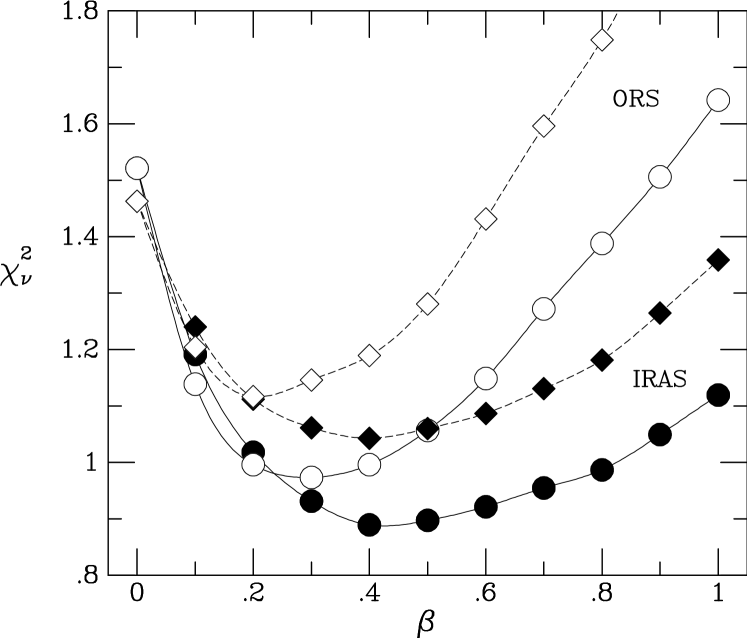
Figure 2.— The reduced $\chi^{2}$ is plotted as a function of $\beta$ for $H_{0}{\,=\,}74$ km s${}^{-1}\,$Mpc and $\sigma_{v}=200$ km s^-1. Circles connected by solid spline curves show results from “Trial 2,” which includes all 280 galaxies, and diamonds connected by dashed curves show results from “Trial 3,” which removes 102 galaxies near the Virgo and Fornax clusters. Solid/open symbols are used for the IRAS/ORS comparisons.

Figure 3 illustrates how the reduced $\chi^{2}$ for $H_{0}=74$ and $\sigma_{v}=200$ varies with $\beta$ for trials 2 and 3 (spanning the range in best-fit $\beta$ and $\chi^{2}_{\nu}$) of the IRAS and ORS comparisons. Overall, the last columns of Table 1 indicate $\beta_{I}=0.42^{+0.10}_{-0.06}$ and $\beta_{O}=0.26\pm 0.08$, where the errors include the uncertainty for a given trial (including the 2% uncertainty in $H_{0}$ from the velocity tie) and the variation among the trials. The results are independent of whether one takes a median or average of the trials, or adopts either $\sigma_{v}=150$ or 200 km s^-1. However, $\beta_{I}$ and $\beta_{O}$ would increase for example by $\sim\,$30% to 0.56 and 0.33, respectively, if $H_{0}$ were known to be 5% larger for a fixed distance zero point, or decrease by 15–20% if $H_{0}$ were 5% smaller, but again, the $\chi^{2}$ analysis indicates $H_{0}$ is constrained to 2% for a fixed distance zero point.

Finally, Figure 3 compares the $\beta_{I}=0.4$ predicted and $H_{0}=74$ observed peculiar velocities in the Local Group frame for all the galaxies, using their group-averaged velocities to limit noise. Given that the two sets of peculiar velocities were derived independently (apart from our adjustment of $H_{0}$ and $\beta_{I}$), the agreement is quite good. The predictions resemble a heavily smoothed version of the observations, and $\chi^{2}_{\nu}$ confirms this, although the residuals may hint at a slightly misaligned dipole. Large negative residuals near $(l,b)\sim(283^{\circ},+74^{\circ})$ indicate Virgo backside infall in excess of what the spherical harmonic solution can produce. These issues will be addressed in more detail by a forthcoming paper (Willick et al. 2000, in preparation).

Figure 3.— Predicted peculiar velocities from the IRAS survey (top) with $\beta_{I}=0.4$, observed peculiar velocities from the SBF survey (middle) with $H_{0}=74$ km s${}^{-1}\,$Mpc, and the residuals (observed minus predicted, bottom) are shown in Galactic coordinates and the Local Group frame. Light/dark circles show negative/positive peculiar velocities, coded in size as shown; smaller symbols are plotted on top of larger ones for clarity. Unlike the predictions, the observations have no smoothing applied and contain both distance and velocity errors, causing the greater range in symbol size.

4. Discussion

We have found the most consistent results for $H_{0}=74$ km s${}^{-1}\,$Mpc, intermediate between the favored values of 77 and 71 reported by SBF-II and the $H_{0}$ Key Project’s analysis of SBF (F99), respectively. The differences in these “SBF $H_{0}$” values result entirely from the flow models. SBF-II explored a number of parametric flow models ranging from a pure Hubble flow plus dipole to models with two massive attractors and a residual quadrupole, as well as some with a local void component. The pure Hubble flow model gave the same $H_{0}$ as obtained by F99. Adding Virgo and Great Attractors gave $H_{0}{\,=\,}73.5$, and the additional Local Group-centered quadrupole gave a further 6% increase in $H_{0}$. Each component significantly improved the model likelihood, but it was suggested that the quadrupole arose from inadequate modeling of the flattened Virgo potential. If so, then $H_{0}$ may be better estimated using a sharply cutoff, Virgo-centered quadrupole. Figure 23 of SBF-II shows that such a model would indeed yield $H_{0}\approx 74$.

We also note that most of the SBF-II models had a significant excess Local Group peculiar motion of $\sim\,$190 km s^-1, unlike the IRAS density field predictions (e.g., Willick etal 1997). However, when the excess was modeled as a “push” from a large nearby void, $H_{0}$ dropped from 78 to 73 because of the underdensity introduced. This model achieved the best likelihood of any considered, but the treatment of the void was deemed too ad hoc to qualify as a standard component of the flow model. Thus, it may be that the SBF-II result for $H_{0}$ suffered from the arbitrariness inherent in parametric modeling. However, the good match we find between the predicted and observed velocity fields supports the claim by SBF-II that, after accounting for the attractor infalls, any bulk flow of the volume $c{z}\mathrel{\hbox to0.0pt{\lower 3.0pt\hbox{$\mathchar 536\relax$}\hss}\raise 2.0pt\hbox{$\mathchar 316\relax$}}3000$ km s^-1 is $\mathrel{\hbox to0.0pt{\lower 3.0pt\hbox{$\mathchar 536\relax$}\hss}\raise 2.0pt\hbox{$\mathchar 316\relax$}}200$ km s^-1, as the structure within this volume accounts for most of our motion in the cosmic microwave background rest frame (see Nusser & Davis 1994).

The best-fit values of $\beta_{I}=0.42^{+0.10}_{-0.06}$ and $\beta_{O}=0.26\pm 0.08$ are similar to the $\beta_{I}=0.40\pm 0.15$ and $\beta_{O}=0.3\pm 0.1$ results found by Riess et al. (1997) using 24 SNIa distances out to $c{z}\sim 9000$ km s^-1, nearly 3 times our survey limit. It is interesting that despite the close agreement on $\beta$, SBF and SNIa still disagree by nearly 10% on $H_{0}$ (e.g., Gibson et al. 1999). This implies that the discrepancy is mainly due to the respective distance calibrations against the Cepheids (otherwise the $H_{0}$ offset would cause major disagreement on $\beta$). We also note that the ratio $\beta_{I}/\beta_{O}\approx 1.6$ agrees well with the estimates by Baker et al. (1998).

Our results are consistent with all other recent comparisons of the gravity and velocity fields (so-called “velocity-velocity” comparisons), regardless of the distance survey used. Thus, the near factor-of-two discrepancy with the Potent analysis (a “density-density” comparison) of Sigad et al. (1998) persists. Since the latter analysis is done at larger smoothing scales, one obvious explanation is non-trivial, scale-dependent biasing, and some simulations may give the needed factor-of-two change in bias over the relevant range of scales (Kauffmann et al. 1997; but see Jenkins et al. 1998). However, at this point, the inconsistency in the results of the two types of analysis remains unexplained.

We are currently in the process of analyzing the SBF data set using methods that deal directly with multivalued redshift zones and incorporate corrections to linear gravitational instability theory to take advantage of SBF’s ability to probe the small-scale nonlinear regime (Willick et al. 2000, in preparation). We also plan in the near future to use the data for a “density-density” determination of $\beta$. In addition, we are working towards a direct, unambiguous tie of SBF to the far-field Hubble flow, which will significantly reduce the systematic uncertainty in $\beta$.

References

- Baker et al. (1998) Baker, J. E., Davis, M., Strauss, M. A., Lahav, O., Santiago, B. X. 1998, ApJ, 508, 6
- Blakeslee, Ajhar, & Tonry (1999) Blakeslee, J. P., Ajhar, E. A., & Tonry, J. L. 1999, in Post-Hipparcos Cosmic Candles, eds. A. Heck & F. Caputo (Boston: Kluwer), 181
- da Costa et al. (1998) da Costa, L. N., Nusser, A., Freudling, W., Giovanelli, R., Haynes, M. P., Salzer, J. J., & Wegner, G. 1998, MNRAS, 299, 425
- Davis et al. (1996) Davis, M., Nusser, A. & Willick, J. A. 1996, ApJ, 473, 22
- Dekel et al. (1990) Dekel, A., Bertschinger, E., & Faber, S. M. 1990, ApJ, 364, 349
- Fadda et al. (1996) Fadda, D., Girardi, M., Giuricin, G., Mardirossian, F., Mezzetti, M. & Biviano, A. 1996, ApJ, 473, 670
- Ferrarese et al. (1999) Ferrarese, L., et al. 1999, ApJ, in press (F99)
- Fisher et al. (1995) Fisher, K. B., Huchra, J. P., Strauss, M. A., Davis, M., Yahil, A., & Schlegel, D. 1995, ApJS, 100, 69
- Gibson et al. (1999) Gibson, B. K., et al. 1999, ApJ, in press
- Girardi et al. (1998) Girardi, M., Giuricin, G., Mardirossian, F., Mezzetti, M., & Boschin, W. 1998, ApJ, 505, 74
- Jenkins et al. (1998) Jenkins, A., et al. 1998, ApJ, 499, 20
- Kauffmann et al. (1997) Kauffmann, G., Nusser, A., & Steinmetz, M. 1997, MNRAS, 286, 795
- Mould et al. (1999) Mould, J. R. et al. 1999, ApJ, in press
- Nusser & Davis (1994) Nusser, A. & Davis, M. 1994, ApJ, 421, L1
- Peebles (1980) Peebles, P.J.E. 1980, The Large Scale Structure of the Universe (Princeton Univ. Press)
- Riess et al. (1997) Riess, A. G., Davis, M., Baker, J., & Kirshner, R. P. 1997, ApJ, 488, L1
- Santiago et al. (1995) Santiago, B. X., Strauss, M. A., Lahav, O., Davis, M., Dressler, A., & Huchra, J. P. 1995, ApJ, 446, 457
- Schlegel (1995) Schlegel, D. J. 1995, Ph.D. Thesis, Univ. of California, Berkeley
- Sigad et al. (1998) Sigad, Y., Eldar, A., Dekel, A., Strauss, M. A., & Yahil, A. 1998, ApJ, 495, 516
- Strauss & Willick (1995) Strauss, M. A. & Willick, J. A. Phys. Rep., 261, 271
- Tonry (1991) Tonry, J. L. 1991, ApJ, 373, L1.
- Tonry et al. (1997) Tonry, J. L., Blakeslee, J. P., Ajhar, E. A., & Dressler, A. 1997, ApJ, 475, 399 (SBF-I)
- Tonry et al. (1999) Tonry, J. L., Blakeslee, J. P., Ajhar, E. A., & Dressler, A. 1999, ApJ, in press (SBF-II)
- Tonry & Schneider (1988) Tonry, J. L. & Schneider, D. P. 1988, AJ, 96, 807
- Willick et al. (1997) Willick, J. A., Strauss, M. A., Dekel, A., & Kolatt, T. 1997, ApJ, 486, 629
- Willick & Strauss (1998) Willick, J. A. & Strauss, M. A. 1998, ApJ, 507, 64