Kepler Rotation Effects
on the Binary-Lens Microlensing Events

Abstract

We investigate the effects of the Kepler rotation of lens binaries on the binary-microlensing events towards the Large Magellanic Cloud (LMC) and the Small Magellanic Cloud (SMC). It is found that the rotation effects cannot always be neglected when the lens binaries are in the LMC disk or the SMC disk, i.e., when they are self-lensing. Therefore we suggest that it will be necessary to consider the rotation effects in the analyses of the coming binary events if the microlensing events towards the halo are self-lensing. As an example, we reexamine the MACHO LMC-9 event, in which the slow transverse velocity of the lens binary suggests a microlensing event in the LMC disk. From a simple analysis, it is shown that the lens binary with total mass $\sim 1M_{\odot}$ rotates by more than $\sim 60^{\circ}$ during the Einstein radius crossing time. However, the fitting of MACHO LMC-9 with an additional parameter, the rotation period, shows that the rotation effects are small, i.e., the projected rotation angle is only $\sim 5.9^{\circ}(M/M_{\odot})^{1/4}$ during the Einstein radius crossing time. This contradiction can be settled if the physical parameters, such as the mass and the velocity, are different in this event, the binary is nearly edge-on, or the binary is very eccentric, though definite conclusions cannot be drawn from this single event. If the microlensing events towards the halo are due to self-lensing, binary-events for which the rotation effects are important will increase and stronger constraints on the nature of the lenses will be obtained.

1 Introduction

The analysis of the first $2.1$ years of photometry of $8.5\times 10^{6}$ stars in the LMC by the MACHO Collaboration [1] suggests that the fraction $0.62^{+0.3}_{-0.2}$ of our halo consists of massive compact halo objects (MACHOs) of mass $0.5^{+0.3}_{-0.2}M_{\odot}$ in the standard spherical flat rotation halo model. A preliminary analysis of four years of data suggests the existence of at least eight additional microlensing events with $t_{\rm dur}\sim 90$ days in the direction of the LMC. [2]

At present, we do not know what MACHOs are. There have been several identifications of MACHOs proposed, such as brown dwarfs, red dwarfs, white dwarfs, neutron stars, primordial black holes, and so on. [2, 3, 4, 5, 6, 7, 8, 9, 10, 11, 12, 13, 14, 15, 16, 17, 18, 19, 20, 21] Any objects clustered somewhere between the LMC and the Sun with column density larger than $25M_{\odot}{\rm pc}^{-2}$ may also explain the data. [22] They include the following possibilities: LMC-LMC self-lensing, the spheroid component, thick disk, a dwarf galaxy, tidal debris, and warping and flaring of the galactic disk. [23, 24, 25, 26, 27, 28, 29] (See also Ref. NI99.)

Such obscurities of the mass and the spatial distribution essentially result from the fact that the time scale of an event, which is an important observable, is a degenerate combination of the three quantities one would like to know, the mass, the velocity and the position of the lensing object. Several methods have been proposed to break these degeneracies, for example, launching a parallax satellite into solar orbit, [31, 32, 33, 34, 35] observing the annual modulation in light magnification induced by the Earth’s motion, [36, 37] observing the deviation of light magnification from a simple point-source model due to the finite-source size effect when the impact parameter of the trajectory of the lens is comparable to the source size, [38, 39, 40] distinguishing the dependence of the lensing rate on the background stellar density, [41] and so on.

A microlensing event due to a binary is one of the best candidates to break the degeneracies. In binary-microlensing events, the light magnification dramatically deviates from that of a simple point-source model when the source transverses the caustics, where a point source is amplified infinitely. We can obtain information concerning the transverse velocity of the source from this deviation, which can be used to distinguish between halo-lensing and self-lensing. To this time, two binary-lens microlensing events have been observed, MACHO LMC-9 [42] and MACHO 98-SMC-1. [43, 44, 45] Although we cannot say for certain from only these events, [46] these events support self-lensing because of slow transverse velocities. In the future, the number of binary-lens microlensing events will increase, [47, 48] and hence these events will be important to break the degeneracies in the physical parameters.

In almost all analyses of binary-lens microlensing events, the rotation of the lens binary has been neglected.[42] This is because the period of a lens binary in the halo is much larger than the time scale of the amplification. However, the lensing object of the MACHO LMC-9 event, for example, is very likely to reside in the LMC disk, not in our halo. Since the characteristic transverse velocity of a lens in the LMC disk or the SMC disk is smaller than that in our halo, the rotation of the lens binary in the disk may be important. For this reason we reconsider the rotation effects on the analyses of the binary-lens microlensing events in this paper. As an example we reanalyze the MACHO LMC-9 event taking the rotation into account. Note that, in the previous analysis of this event, the transverse velocity is somewhat smaller than that expected for a lens in the LMC disk.[42] If we take the rotation of the lens binary into account, the transverse velocity may be larger, since the incident angle of the trajectory of the source into the caustics may be smaller, and hence the source may take shorter time to move by one stellar radius of the source. This is one of our motivations to examine the rotation effects.

In §2 microlensing by a double point mass is reviewed. In §3 the rotation effects of a lens binary are estimated. We suggest the possibility that the rotation effects are important when the lens binary resides in the LMC disk or the SMC disk. In §4 we perform the fitting of the MACHO LMC-9 event, taking into account the rotation of the lens binary. Section 5 is devoted to summary and discussion.

2 Microlensing by two point masses

We now briefly review microlensing by a double point mass [49, 50] to introduce our notation. We consider a lens binary consisting of two point masses, $M_{1}$ and $M_{2}$, whose center is at a distance $D_{ol}$ from the observer, and we consider a source at a distance $D_{os}$ from the observer in Fig. 1. We define the lens plane as the plane which contains the center of mass of the lens binary and is perpendicular to the line connecting the observer and the center of mass, i.e., the optical axis. We also define the source plane as the plane which contains the source and is parallel to the lens plane. The distance between the lens plane and the source plane is written as $D_{ls}=D_{os}-D_{ol}$. We define a coordinate system $(\xi_{x},\xi_{y})$ on the lens plane and $(\eta_{x},\eta_{y})$ on the source plane, taking the origin of each coordinate at the intersection between each plane and the optical axis. An equation which relates the image position $\xi$ to the source position $\eta$ is called a “lens equation”. From Fig. 1, we see that the lens equation for lensing by a double point mass is

$$\eta = {{D_{os}}\over{D_{ol}}}{\mbox{\boldmath$\xi$}}-{D_{ls}}{\mbox{{\boldmath$\Theta$}}}({\mbox{\boldmath$\xi$}}),$$ (1)

$${\mbox{{\boldmath$\Theta$}}}({\mbox{\boldmath$\xi$}}) = {{4GM_{1}}\over{c^{2}}}{{{\mbox{\boldmath$\xi$}}-{\mbox{\boldmath$\xi$}}_{1}}\over{|{\mbox{\boldmath$\xi$}}-{\mbox{\boldmath$\xi$}}_{1}|^{2}}}+{{4GM_{2}}\over{c^{2}}}{{{\mbox{\boldmath$\xi$}}-{\mbox{\boldmath$\xi$}}_{2}}\over{|{\mbox{\boldmath$\xi$}}-{\mbox{\boldmath$\xi$}}_{2}|^{2}}},$$ (2)

where ${\mbox{\boldmath$\xi$}}_{1}$ and ${\mbox{\boldmath$\xi$}}_{2}$ are the positions of the masses projected onto the lens plane. ${\mbox{{\boldmath$\Theta$}}}({\mbox{\boldmath$\xi$}})$ is the deflection angle of light due to the lens masses, which is the summation of the deflection angle due to each mass. The Einstein radius for the total mass of the binary, $M=M_{1}+M_{2}$, is defined as

$$\rho_{E}:=\sqrt{{{4GM}\over{c^{2}}}{{D_{ol}D_{ls}}\over{D_{os}}}}=\sqrt{{{4GMD_{os}}\over{c^{2}}}x(1-x)},$$ (3)

where $x:={{D_{ol}}/{D_{os}}}$. With the definitions

$${\mbox{{\boldmath$r$}}}:={{\mbox{\boldmath$\xi$}}\over{\rho_{E}}},\quad{\mbox{{\boldmath$z$}}}:=x{{\mbox{\boldmath$\eta$}}\over{\rho_{E}}},\quad\mu_{i}:={{M_{i}}\over M},\quad{(i=1,2)}$$ (4)

the lens equations (1) and (2) become dimensionless equations,

$$z = {\mbox{{\boldmath$r$}}}-{\mbox{{\boldmath$\Theta$}}}({\mbox{{\boldmath$r$}}}),$$ (5)

$${\mbox{{\boldmath$\Theta$}}}({\mbox{{\boldmath$r$}}}) = \mu_{1}{{{\mbox{{\boldmath$r$}}}-{\mbox{{\boldmath$r$}}}_{1}}\over{|{\mbox{{\boldmath$r$}}}-{\mbox{{\boldmath$r$}}}_{1}|^{2}}}+\mu_{2}{{{\mbox{{\boldmath$r$}}}-{\mbox{{\boldmath$r$}}}_{2}}\over{|{\mbox{{\boldmath$r$}}}-{\mbox{{\boldmath$r$}}}_{2}|^{2}}}.$$ (6)

Note that we are discussing the situation on the lens plane, since we normalize the length as in Eq. (4).

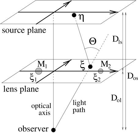
Figure 1: The geometry of the gravitational lensing by a double point mass lens.

These equations (5) and (6) can be used to find all images of the source. [51] If we cannot resolve the images by observations, the only observable quantity is the amplification of the brightness of the source. The amplification factor $I$ is the inverse of the determinant of the Jacobi matrix,

$$I=\sum_{i}\left.\left|\det\left({{\partial{\mbox{{\boldmath$z$}}}}\over{\partial{\mbox{{\boldmath$r$}}}}}\right)\right|^{-1}\right|_{{\mbox{{\boldmath$r$}}}={\mbox{{\boldmath$r$}}}_{i}},$$ (7)

where ${\mbox{{\boldmath$r$}}}_{i}$ is the image position. For certain values of $r$, the amplification factor $I$ diverges. A set of these points forms curves called “critical curves”. The projection of the critical curves onto the source plane with Eqs. (5) and (6) forms caustics on the source plane. Caustics have three kinds of morphology, depending on the separation of the masses. In Fig. 2 these three kinds of caustics are shown. The number of images is five in the closed caustics and three outside. Around the caustics, large amplification appears, and the light curve has a peak.

Figure 2: Caustics for a double point lens. The lenses have identical masses and are separated by $l=0.6,1.4$ and $2.2$.

3 Microlensing events by a binary lens

3.1 Motion of the source

We assume that we can neglect the Earth’s motion around the Sun, and consider the relative motion of the observer, the lens and the source as the motion of the source. Every quantity on the source plane is projected onto the lens plane by Eq. (4). Hence it is convenient to consider the motion of the source as that projected onto the lens plane with Eq. (4). The trajectory of the source is characterized by its impact parameter $b$ with respect to the origin of the lens plane in units of the Einstein radius $\rho_{E}$ and the angle $\theta$ between the $x$-axis on the lens plane and the trajectory. The source closest approaches the origin at $T_{S}$, and the transverse velocity of the source in the lens plane is $V_{\bot}$. The transverse velocity of the source pulled back onto the source plane $V_{T}$ is related to $V_{\bot}$ as

$$V_{T}={{V_{\bot}}\over{x}}.$$ (8)

The Einstein radius crossing time $t_{E}$ is defined as

$$t_{E}:={{\rho_{E}}\over{V_{\bot}}}.$$ (9)

It is convenient to measure the time $T$ with respect to $t_{E}$, $t:={{T}/{t_{E}}}$. By normalizing the time in this manner, the source moves by a unit length in a unit time. The source closest approaches the origin at the normalized time, $t_{S}:=T_{S}/t_{E}$.

If there are enough data around the peak of the light curve, important information about the size of the source can be obtained. [42] If the radius of the source is $R_{\star}$, it takes a time

$$T_{\star}={{R_{\star}}\over{V_{T}}}=x{{R_{\star}}\over{V_{\bot}}}$$ (10)

for the source to move by one stellar radius of the source.

3.2 Rotation of the lens binary

The lens binary rotates according to Kepler’s law. The relative vector $U$ is defined by ${\mbox{{\boldmath$U$}}}:={\mbox{{\boldmath$U$}}}_{1}-{\mbox{{\boldmath$U$}}}_{2}$, where ${\mbox{{\boldmath$U$}}}_{1}$ and ${\mbox{{\boldmath$U$}}}_{2}$ denote the positions of the binary masses in the orbital plane. We take the origin of the orbital plane at the center of the binary masses as $M_{1}{\mbox{{\boldmath$U$}}}_{1}+M_{2}{\mbox{{\boldmath$U$}}}_{2}=0$. Hence, the positions of the binary masses are determined by the relative vector $U$ as ${\mbox{{\boldmath$U$}}}_{1}={\mu_{2}}{\mbox{{\boldmath$U$}}}$ and ${\mbox{{\boldmath$U$}}}_{2}=-{\mu_{1}}{\mbox{{\boldmath$U$}}}$, where $\mu_{1}$ and $\mu_{2}$ are defined in Eq. (4). In the orbital plane, the relative vector ${\mbox{{\boldmath$U$}}}=(U\cos\phi,U\sin\phi)$ at a time $T$ is determined through the parameter $\lambda$ as

$$T-T_{0} = {{T_{B}}\over{2\pi}}(\lambda-e\sin\lambda),$$ (11)

$$U = A(1-e\cos\lambda),$$ (12)

$$\cos(\phi-\phi_{0}) = {{\cos\lambda-e}\over{1-e\cos\lambda}},$$ (13)

where

$$T_{B}=2\pi\sqrt{{{A^{3}}\over{GM}}}$$ (14)

is the period, $A$ is the semi-major axis, and $e$ is the eccentricity of the lens binary. $T_{0}$ and $\phi_{0}$ are integral constants. We can take the coordinates on the orbital plane so that $\phi_{0}=0$. With the definitions

$$t_{B}:={{T_{B}}\over{t_{E}}},\quad t_{0}:={{T_{0}}\over{t_{E}}},\quad{\mbox{{\boldmath$u$}}}:={{\mbox{{\boldmath$U$}}}\over{\rho_{E}}},\quad a:={{A}\over{\rho_{E}}},$$ (15)

the above equations (11), (12) and (13) become dimensionless:

$$t-t_{0} = {{t_{B}}\over{2\pi}}(\lambda-e\sin\lambda),$$ (16)

$$u = a(1-e\cos\lambda),$$ (17)

$$\cos\phi = {{\cos\lambda-e}\over{1-e\cos\lambda}}.$$ (18)

In general, the orbital plane does not coincide with the lens plane. Since we consider the case $D_{ol}\gg A$, it is convenient to think about the lens masses projected onto the lens plane, i.e., the thin lens approximation. The orientation of the coordinates in the orbital plane relative to the coordinates in the lens plane is determined by Euler angles $\alpha$, $\beta$ and $\gamma$. In Fig. 3, we show the relation between the orbital plane and the lens plane, where $(r_{x},r_{y})$ plane is the lens plane, $(u_{x},u_{y})$ plane is the orbital plane, and $\alpha$, $\beta$ and $\gamma$ are Euler angles. We can take the coordinates in the lens plane so that $\alpha=0$, since $\alpha$ can be absorbed into $\theta$, the angle between the $x$-axis in the lens plane and the trajectory of the source. A point $(u\cos\phi,u\sin\phi)$ in the orbital plane is projected to the point $({l}\cos\varphi,{l}\sin\varphi)$ in the lens plane, where

$$l = u\sqrt{\cos^{2}\beta\cos^{2}(\phi+\gamma)+\sin^{2}(\phi+\gamma)},$$ (19)

$$\tan\varphi = {{\tan(\phi+\gamma)}\over{\cos\beta}}.$$ (20)

Figure 3: The relation between the orbital plane and the lens plane. The $(r_{x},r_{y})$ plane is the lens plane, the $(u_{x},u_{y})$ plane is the orbital plane, and $\alpha$, $\beta$ and $\gamma$ are Euler angles.

3.3 Estimate of the rotation effects

We can estimate the rotation effects of a lens binary by comparing the period of the binary $T_{B}$ with the Einstein radius crossing time $t_{E}$. If the ratio $t_{B}={{T_{B}}/{t_{E}}}$, is not much larger than unity, we cannot neglect the rotation of the binary.

For a typical MACHO, the ratio $t_{B}$ is given by

$$t_{B}={{T_{B}}\over{t_{E}}}={{2\pi V_{\perp}}\over{\rho_{E}}}\sqrt{{A^{3}}\over{GM}}={{2\pi V_{\perp}}\over{\rho_{E}}}\sqrt{{\rho_{E}^{3}a^{3}}\over{GM}}$$ (21)

$$\sim 134\left({{a}\over{1}}\right)^{3/2}\left({{D_{OS}}\over{50\ {\rm kpc}}}\right)^{1/4}\left({{M}\over{M_{\odot}}}\right)^{-1/4}\left({{V_{\perp}}\over{200\ {\rm km/s}}}\right)\left({{x(1-x)}\over{0.5(1-0.5)}}\right)^{1/4},$$

using Eqs. (3), (9), (14) and (15). This implies that a typical binary in our halo rotates by about $360^{\circ}/t_{B}\simeq 2.7^{\circ}(M/M_{\odot})^{1/4}$ during the Einstein radius crossing time. This may be small enough to neglect the rotation of the binary.

On the other hand, if a lens binary resides in the LMC disk, the parameters are different. For a typical LMC lens, assuming that the thickness of the LMC disk is smaller than $\sim 500$ pc, the ratio $t_{B}$ is given by

$$t_{B}\mathrel{\mathchoice{\lower 2.15277pt\vbox{\halign{$\mathsurround 0pt \displaystyle\hfil#\hfil$\cr<\crcr\sim\crcr}}}{\lower 2.15277pt\vbox{\halign{$\mathsurround 0pt \textstyle\hfil#\hfil$\cr<\crcr\sim\crcr}}}{\lower 2.15277pt\vbox{\halign{$\mathsurround 0pt \scriptstyle\hfil#\hfil$\cr<\crcr\sim\crcr}}}{\lower 2.15277pt\vbox{\halign{$\mathsurround 0pt \scriptscriptstyle\hfil#\hfil$\cr<\crcr\sim\crcr}}}}18\left({{a}\over{1}}\right)^{3/2}\left({{D_{OS}}\over{50\ {\rm kpc}}}\right)^{1/4}\left({{M}\over{M_{\odot}}}\right)^{-1/4}\left({{V_{\perp}}\over{60\ {\rm km/s}}}\right)\left({{x(1-x)}\over{0.99(1-0.99)}}\right)^{1/4},$$ (22)

which implies that the binary rotates by more than $\sim 20^{\circ}(M/M_{\odot})^{1/4}$ during the Einstein radius crossing time. Thus, if the lens resides in the LMC disk, the rotation effects may be important for the fitting of the light curve. This argument can also be applied to an SMC lens, since the transverse velocity is small and $x$ is close to 1.

Bennett et al. [42] fitted the data of MACHO LMC-9 and obtained fitted parameters as in Table 1. The radius of the source is estimated as

$$R_{\star}=1.5\pm 0.2\ {\rm R_{\odot}},$$ (23)

using the theory of stellar evolution. The transverse velocity in the source plane can be estimated as

$$V_{T}={{R_{\star}}\over{T_{\star}}}=19\pm 6\ {\rm km/s},$$ (24)

with $T_{\star}$ in Table 1 and Eq. (10). Comparing this value with the probability distribution of the transverse velocity in the LMC disk and the Milky Way halo, a lens in the LMC disk is preferred over a halo lens.[42] Assuming that the lens of MACHO LMC-9 resides in the LMC disk, the ratio $t_{B}$ is given by

$$t_{B}<5.7\left({{a}\over{1}}\right)^{3/2}\left({{D_{OS}}\over{50\ {\rm kpc}}}\right)^{1/4}\left({{M}\over{M_{\odot}}}\right)^{-1/4}\left({{V_{\perp}}\over{19\ {\rm km/s}}}\right)\left({{x(1-x)}\over{0.99(1-0.99)}}\right)^{1/4},$$ (25)

where we use the relation $V_{\bot}<V_{T}$, since $V_{\bot}=xV_{T}$ and $x<1$. Since Eq. (25) indicates that the binary rotates by more than $\sim 60^{\circ}(M/M_{\odot})^{1/4}$ during the Einstein radius crossing time, we cannot neglect the rotation of the binary for the fitting of the data. Therefore we perform the fitting of the MACHO LMC-9 event taking into account the rotation of the lens binary in the next section.

The conclusion of this section is that the rotation effects cannot be always neglected when the lens binaries are in the LMC disk or the SMC disk, while the rotation can be neglected when the lenses are in the Milky Way halo.

4 Fitting of the observed data in the binary-lens events

4.1 Parameters characterizing the binary-lens microlensing events

We summarize the parameters necessary to describe the binary-lens microlensing event in this section. First, a dual color observation requires two parameters, taking the blending into consideration:

• $f_{oR}$ : fraction of the lensed brightness of the lensed star in the red band.

• $f_{oB}$ : fraction of the lensed brightness of the lensed star in the blue band.

When we can neglect the rotation of the lens binary, we need the following parameters:

• $t_{E}$ : Einstein radius crossing time.

• $T_{S}$ : time when the source most closely approaches the origin.

• $b$ : impact parameter of the source in the lens plane in units of the Einstein radius.

• $\theta$ : angle between the $x$-axis in the lens plane and the trajectory of the source.

• $\mu_{1}$ : the mass fraction of the first mass.

• $l$ : separation of the lens masses projected onto the lens plane in units of the Einstein radius.

• $T_{\star}$ : time for the source to move by one stellar radius of the source.

If we can neglect the finite size of the source, the last parameter $T_{\star}$ is not necessary.

When we consider the rotation of the lens binary, we need the following parameters in addition to the above parameters:

• $a$ : semi-major axis of the lens binary in units of the Einstein radius.

• $t_{B}$ : period of the lens binary in units of the Einstein radius crossing time.

• $\beta$ : Euler angle.

• $\gamma$ : Euler angle.

• $e$ : eccentricity of the lens binary.

• $T_{0}$ : time when the binary is at the pericenter.

where the parameter (8) has been replaced. We need five additional parameters when we take the rotation of the lens binary into account.

If we assume that the orbit of the binary is circular ($e=0$), the parameters (13) and (14) are not necessary, since $T_{0}$ can be absorbed into $\gamma$. If we assume that the orbit of the binary is face-on, the parameters (11) and (12) are not necessary, since $\gamma$ can be absorbed into $\theta$. If we assume that the lens binary is face-on and $e=0$, the parameters from (11) to (14) are not necessary.

4.2 Fitting of the MACHO LMC-9 event

We analyze the raw data for the MACHO LMC-9 event. The baseline of the photometry that corresponds to no amplification has to be determined by the fitting with it added as one more parameter. However, to save time, we determine the baseline by the least squares fitting of the data for $T<300$ day and $900$ day $<T$, where the amplification is expected to be less than $(4^{2}+2)/(4\times\sqrt{4^{2}+4})\sim 1.006$. With this baseline we can translate the raw data into the data for the amplification.

We first performed the fitting of the data of MACHO LMC-9 neglecting the rotation of the lens binary to check our fitting code. The result of the $\chi^{2}$ fit is shown in Table 2. This result does not differ greatly from the result in Table 1, which is a crosscheck of our fitting code. The structure of the caustics and the trajectory of the source are shown in Fig. 4. The corresponding light curves are also shown.

Figure 4: The structure of the caustics and the trajectory of the source are shown (left). The corresponding light curves for red (middle) and blue (right) are also shown. The rotation effects are not included.

Next we performed the fitting of the data of MACHO LMC-9 taking account of the rotation of the lens binary. The influence of the rotation of the lens binary on the light curve can be divided into two effects, the change of the caustics shape with time caused by the change of $l$ and rotation of the caustics with time in the lens plane, which is treated as a curve of the source trajectory. However, since the former effect is hardly separated from the ambiguity of the other parameters within the limited accuracy of the observation, we consider only the latter effect. Thus, in order to evaluate the rotation effects, it is useful to examine the case that the binary is face-on and $e=0$. Therefore we assume that the binary is face-on and $e=0$ as a first step. Then we need ten parameters, (1)-(10) in §4.1. The results of the $\chi^{2}$ fitting are shown in Table 3. The structure of the caustics and the trajectory of the source are shown in Fig. 5. The corresponding light curves are also shown.

Contrary to our expectations, there are few differences between the fitted parameters with and without the rotation from Tables 2 and 3. This is because the period of the lens binary $t_{B}$ is quite large. The binary rotates by only $\sim 5.9^{\circ}(M/M_{\odot})^{1/4}$ during the Einstein radius crossing time. Thus the rotation effects are very small. Note that the result of the small rotation effects does not depend on the face-on and $e=0$ assumptions. We can consider the following three possible reasons for the contradiction of the simple estimate of $t_{B}$ in Eq. (22) and the fitted value of $t_{B}$ in Table 3:

1. The physical parameters in Eq. (3.15), such as the mass $M$ and the velocity $V_{\bot}$, are not typical in this event.

2. The binary of this event is nearly edge-on.

3. The binary of this event is very eccentric.

We consider the possible physical parameters that account for the small rotation effects in §4.3, we consider the possible inclination in §4.4, and we consider the possible eccentricity in §4.5.

Figure 5: The structure of the caustics and the trajectory of the source (left). The corresponding light curves for red (middle) and blue (right) are also shown. The rotation effects are included.

4.3 The mass, the velocity and the distance of the lens

Assuming that the binary is face-on and that $e=0$, we can obtain the mass, the velocity and the position of the lens from only the fitted parameters in Table 3 and the radius of the source in Eq. (23) as follows.[55] Note that the probability distribution of the transverse velocity is not necessary.

We assume that the binary is face-on and that $e=0$. The velocity of the lens $V_{\bot}$ is determined by Eq. (10) as

$$V_{\bot}=x{{R_{\star}}\over{T_{\star}}}$$ (26)

for given $x$. Using Eqs. (3), (9) and (26), the total mass of the lens $M$ is determined by

$$M={{c^{2}R_{\star}^{2}}\over{4GD_{os}}}\left({{t_{E}}\over{T_{\star}}}\right)^{2}{{x}\over{1-x}}$$ (27)

for given $x$. Using Eqs. (3), (9), (14), (15) and (26), the position of the lens $x$ is obtained from

$$x^{2}(1-x)={{t_{B}^{2}}\over{16\pi^{2}a^{3}}}{{c^{2}t_{E}T_{\star}}\over{D_{os}R_{\star}}}.$$ (28)

The left-hand side of this equation, $f(x):=x^{2}(1-x)$, is plotted in Fig. 6. The function $f(x)$ has a maximum value $f(2/3)=4/27$ at $x=2/3$. The equation $f(x)=y$ has two solutions, $x_{1}$ and $x_{2}$, for $0<y<4/27$. The right-hand side of Eq. (28) is determined from the fitted parameters.

After determining the positions, $x_{1}$ and $x_{2}$, with Eq. (28), we can obtain the mass and the velocity of the lens for each distance with Eqs. (26) and (27). Since the right-hand side of Eq. (28) is 0.0860 from Table 3, two solutions of this equation are

$$x_{1}=0.369\quad{\rm and}\quad x_{2}=0.892.$$ (29)

The corresponding mass and velocity are

$$M=0.000902\ M_{\odot},\quad V_{\bot}=7.30\ {\rm km/s}\quad{\rm for}\ x=x_{1},$$ (30)

$$M=0.0127\ M_{\odot},\quad V_{\bot}=17.6\ {\rm km/s}\quad{\rm for}\ x=x_{2}.$$ (31)

If the binary of the MACHO LMC-9 event has such physical parameters, we can explain the small rotation effects. However, these parameters seem to be quite strange. The mass seems to be too small, and the position favors the halo lens, while the transverse velocity prefers the LMC lens. However, we cannot draw definite conclusions from this event alone.

Figure 6: $f(x)=x^{2}(1-x)$. The horizontal dotted line is the right-hand side of Eq. ($5\cdot 3$) with the fitted parameters in Table III.

4.4 Inclination

In this section we consider a possible inclination to explain the small rotation effects in the MACHO LMC-9 event. Without the face-on assumption, the fitted values of $t_{B}$ and $a$ do not generally coincide with the real values of $t_{B}$ and $a$. We obtained the mass, the velocity and the position using $\tilde{t}_{B}$ and $\tilde{a}$ instead of $t_{B}$ and $a$, respectively, in Eq. (28), where $\tilde{t}_{B}$ and $\tilde{a}$ denote the fitted values of $t_{B}$ and $a$, respectively. Therefore a certain inclination may explain the small rotation effects even if we use typical physical parameters. To investigate the inclination effect, we set $e=0$. Therefore the additional parameters are the Euler angles $\beta$ and $\gamma$, as shown in §4.1. Rigorously, the parameters $t_{B}$ and $a$ for given $\beta$ and $\gamma$ have to be determined by the fitting. However, we can approximately determine $t_{B}$ and $a$ for given $\beta$ and $\gamma$ from $\tilde{t}_{B}$ and $\tilde{a}$ as follows.

Assuming that $\tilde{a}$ is mainly determined by the separation between the projected masses at $t=t_{S}$, the relation between $a$ and $\tilde{a}$ can be estimated by Eq. (19) as

$$a={{\tilde{a}}\over{\sqrt{\cos^{2}\beta\cos^{2}\gamma+\sin^{2}\gamma}}},$$ (32)

since $\phi=0$ at $t=t_{S}$ when $e=0$. To determine the relation between $t_{B}$ and $\tilde{t}_{B}$, we assume that the parameter $\tilde{t}_{B}$ is mainly determined by the rotation angle projected on the lens plane. In other wards, the relation between $t_{B}$ and $\tilde{t}_{B}$ is determined by the condition that the projection of the rotation angle $4\pi/t_{B}$ between $t=t_{S}-1$ and $t=t_{S}+1$ coincides with $4\pi/\tilde{t}_{B}$. The angle between the relative vector of the binary masses $U$ and the $x$-axis of the orbital plane at $t=t_{S}-1$ is $\phi_{1}:=-2\pi/t_{B}$. The corresponding angle $\varphi_{1}$ between the relative vector projected on the lens plane and the $x$-axis of the lens plane is determined by Eq. (20) as

$$\tan\varphi_{1}={{\tan(\phi_{1}+\gamma)}\over{\cos\beta}}.$$ (33)

Similarly, since the angle between the relative vector of the binary masses $U$ and the $x$-axis of the orbital plane at $t=t_{S}+1$ is $\phi_{2}=2\pi/t_{B}$, the corresponding angle $\varphi_{2}$ between the relative vector projected on the lens plane and the $x$-axis of the lens plane is determined by Eq. (20) as

$$\tan\varphi_{2}={{\tan(\phi_{2}+\gamma)}\over{\cos\beta}}.$$ (34)

The relation between $t_{B}$ and $\tilde{t}_{B}$ is determined by the condition $|\varphi_{2}-\varphi_{1}|=4\pi/\tilde{t}_{B}$. With Eqs. (33) and (34) this relation can be obtained as

$${{2\pi}\over{t_{B}}}=\arctan\left[{{\mp\cos\beta+\sqrt{\cos^{2}\beta+\cos^{4}\gamma(\cos^{2}\beta+\tan^{2}\gamma)(\cos^{2}\beta\tan^{2}\gamma+1)\tan^{2}(4\pi/\tilde{t}_{B})}}\over{\cos^{2}\gamma(\cos^{2}\beta\tan^{2}\gamma+1)\tan(4\pi/\tilde{t}_{B})}}\right],$$

(35)

where the minus sign is for $0<\beta<\pi/2$ and the plus sign is for $\pi/2<\beta<\pi$.

Of course, we cannot determine $\beta$ and $\gamma$ by the fitted parameters. However, inversely, we can determine the allowed region of $\beta$ and $\gamma$ for given $x$. For example, if we assume that the lensing object resides in the LMC disk, i.e.,

$$0.99<x<1,$$ (36)

the left-hand side of Eq. (28) is less than $0.009801$. Substituting Eqs. (32) and (35) into Eq. (28), the allowed region of $\beta$ and $\gamma$ can be obtained in Fig. 7. The probability that the inclination and the phase are in the allowed region is $26.0\%$, assuming random inclination and phase. The corresponding mass and velocity can be obtained by Eqs. (26) and (27) as

$$0.153\ {\rm}M_{\odot}<M,\quad 19.6\ {\rm km/s}<V_{\perp}<19.8\ {\rm km/s}.$$ (37)

In this way, if the binary of this event is nearly edge-on, we can explain the small rotation effects with typical physical parameters. However, we cannot draw definite conclusions from only this event.

Figure 7: The allowed region of the inclination $\beta$ and the phase $\gamma$ for $0.99<x<1$.

4.5 Eccentricity

In this section we consider a possible eccentricity to explain the small rotation effects in the MACHO LMC-9 event. As in the previous section, without the $e=0$ assumption, the fitted values $\tilde{t}_{B}$ and $\tilde{a}$ do not generally coincide with the real values of $t_{B}$ and $a$. Since we use $\tilde{t}_{B}$ and $\tilde{a}$ instead of $t_{B}$ and $a$ in Eq. (28) to obtain the physical parameters, a certain eccentricity may explain the small rotation effects even if we use typical physical parameters. To investigate the eccentricity effect we consider the face-on binary. Therefore, the additional parameters are $e$ and $T_{0}$, as shown in §4.1. We can approximately determine $t_{B}$ and $a$ for given $e$ and $T_{0}$ from $\tilde{t}_{B}$ and $\tilde{a}$ as follows.

Assuming that $\tilde{a}$ is mainly determined by the separation between the projected masses at $t=t_{S}$, the relation between $a$ and $\tilde{a}$ can be approximated by

$$a={{{\tilde{a}}(1+e\cos\phi_{3})}\over{1-e^{2}}},$$ (38)

from Eqs. (17) and (18), where $\phi_{3}$ is determined from Eqs. (16) and (18) with $t=t_{S}$. To determine the relation between $t_{B}$ and $\tilde{t}_{B}$, we assume that the parameter $\tilde{t}_{B}$ is mainly determined by the rotation angle projected on the lens plane. In other words, the relation between $t_{B}$ and $\tilde{t}_{B}$ is determined by the condition that the rotation angle between $t=t_{S}-1$ and $t=t_{S}+1$ coincide with $4\pi/\tilde{t}_{B}$. The angle $\phi_{4}$ between the relative vector between the masses and the $x$-axis of the lens plane at $t=t_{S}-1$ is determined by

$$t_{S}-1-t_{0} = {{t_{B}}\over{2\pi}}(\lambda_{4}-e\sin\lambda_{4}),$$ (39)

$$\cos\phi_{4} = {{\cos\lambda_{4}-e}\over{1-e\cos\lambda_{4}}},$$ (40)

from Eqs. (16) and (18). Similarly, the angle $\phi_{5}$ between the relative vector between the masses and the $x$-axis of the lens plane at $t=t_{S}+1$ is determined by

$$t_{S}+1-t_{0} = {{t_{B}}\over{2\pi}}(\lambda_{5}-e\sin\lambda_{5}),$$ (41)

$$\cos\phi_{5} = {{\cos\lambda_{5}-e}\over{1-e\cos\lambda_{5}}}.$$ (42)

The relation between $t_{B}$ and $\tilde{t}_{B}$ is determined by the condition $\phi_{5}-\phi_{4}=4\pi/\tilde{t}_{B}$. Subtracting Eq. (39) from Eq. (41), we can determine $t_{B}$ as

$${{2\pi}\over{t_{B}}}=Y-e\cos X\sin Y,$$ (43)

where $X:=(\lambda_{4}+\lambda_{5})/2$ and $Y:=(\lambda_{5}-\lambda_{4})/2$ are determined by

$$t_{S}-t_{0}={{X-e\sin X\cos Y}\over{Y-e\cos X\sin Y}},$$ (44)

from Eqs. (39) and (41), and

$$\cos\left({{4\pi}\over{\tilde{t}_{B}}}\right)={{e^{2}\cos^{2}X+(2-e^{2})\cos^{2}Y-2e\cos X\cos Y+e^{2}-1}\over{e^{2}(\cos^{2}X+\cos^{2}Y)-2e\cos X\cos Y+1-e^{2}}},$$ (45)

from Eqs. (40) and (42) and the condition $\phi_{5}-\phi_{4}=4\pi/\tilde{t}_{B}$.

Figure 8: The allowed region of the eccentricity $e$ and $t_{S}-t_{0}\ ({\rm mode}\ t_{B})$ for $0.99<x<1$.

We assume that the lensing object resides in the LMC in Eq. (36). Substituting Eqs. (38) and (43) into Eq.(28), the allowed region of $e$ and $t_{S}-t_{0}\ ({\rm mode}\ t_{B})$ can be obtained in Fig. 8. The minimum eccentricity of this allowed region is 0.892. The corresponding mass and velocity are in Eq. (37). In this way, if the binary of this event is very eccentric, we can explain the small rotation effects with typical physical parameters. However we cannot say for certain from only this event.

5 Summary and discussion

We investigated the rotation effects of lens binaries on the binary-microlensing events towards the LMC and SMC. It is found that the rotation effects cannot always be neglected when the lens binaries are in the LMC disk or the SMC disk, while the rotation can be neglected when the lenses are in our halo. It follows from this that we need to consider the rotation effects in the analyses of the coming binary events if the microlensing events towards the Magellanic Clouds are self-lensing.

In the MACHO LMC-9 event the transverse velocity prefers the lens binary in the LMC disk.[42] For this reason, we reexamined this event in detail as an example. The simple estimate in Eq. (25) indicates that the binary rotates by more than $\sim 60^{\circ}(M/M_{\odot})^{1/4}$ during the Einstein radius crossing time. Therefore we cannot neglect the rotation of the lens binary in the fitting of MACHO LMC-9. We performed the fitting of MACHO LMC-9 taking the rotation into account on the assumption that the binary is face-on and that $e=0$.

Contrary to our expectation, the rotation effects are small, i.e., the projected rotation angle is only $\sim 5.9^{\circ}(M/M_{\odot})^{1/4}$ during the Einstein radius crossing time. Note that this result does not depend on the face-on and $e=0$ assumptions. We can consider three possible reasons for this contradiction between the simple estimate of $t_{B}$ in Eq. (25) and the fitted value of $t_{B}$ in Table 3. The first possibility is that the physical parameters in Eq. (25) are different in this event as in Eqs. (29)-(31), although these parameters are quite peculiar. The second possibility is that the binary of this event is nearly edge-on with typical physical parameters $0.99<x<1$ and Eq.(37), as shown in Fig. 7, although the probability of $\beta$ and $\gamma$ being in the allowed region is only $26\%$ assuming random inclination and phase. The third possibility is that the binary of this event is very eccentric with typical physical parameters $0.99<x<1$ and Eq. (37), as shown in Fig. 8, although the minimum eccentricity of the allowed region is 0.892. However, since we cannot determine all physical parameters including the inclination and the eccentricity only from the light curve, we cannnot draw definite conclusions from only this event.

The transverse velocity is somewhat smaller than that expected for a lens in the LMC disk. This result is the same as that of the analysis of Bennett et al.,[42] even if we take the rotation of the lens binary into account. Since the incident angle of the trajectory of the source into the caustics is not greatly changed, the transverse velocity remains small.

The fitted parameters only represent a local minimum. However, the complete analysis is difficult, since the number of data points around the peak of the light curve is so small that there will be many local minima.[54] The lack of data also allows the possibility that the source is a binary, as Bennett et al. [42] claimed. We agree that it is important to determine whether the source is a binary or not with HST. In order not to overlook the important information from the caustic crossing events, it is necessary to monitor the events frequently, such as with the MOA collaboration [56] and the Alert system.

Note that the rotation effects are not always important when the lens is in the LMC disk or the SMC disk. For example, in the MACHO 98-SMC-1 event the transverse velocity is larger than $\sim 60$ km/s.[43, 44, 45] Since $t_{B}\mathrel{\mathchoice{\lower 2.15277pt\vbox{\halign{$\mathsurround 0pt \displaystyle\hfil#\hfil$\cr>\crcr\sim\crcr}}}{\lower 2.15277pt\vbox{\halign{$\mathsurround 0pt \textstyle\hfil#\hfil$\cr>\crcr\sim\crcr}}}{\lower 2.15277pt\vbox{\halign{$\mathsurround 0pt \scriptstyle\hfil#\hfil$\cr>\crcr\sim\crcr}}}{\lower 2.15277pt\vbox{\halign{$\mathsurround 0pt \scriptscriptstyle\hfil#\hfil$\cr>\crcr\sim\crcr}}}}20\gg 1$ from Eq. (22), the rotation effects are not efficient in this event. Our statement is that there is a sufficient probability that the rotation effects are important for self-lensing.

If the microlensing events towards the halo are due to self-lensing,[23, 24] the number of binary-events for which the rotation effects are important will increase. We will be able to crosscheck whether or not the microlensing events are self-lensing by examining the rotation effects, together with the transverse velocity distribution. As the number of binary-lens events increases, stronger constraints on the nature of the lenses will be obtained statistically.

Appendix A Notations

• : image position in the lens plane

• : source position in the source plane

• : positions of the masses of the lens binary in the lens plane

• : image position in the lens plane in units of $\rho_{E}$

• : source position in the source plane in units of $\rho_{E}$

• : positions of the masses of the lens binary in the lens plane in units of $\rho_{E}$

• : relative vector between the lens masses in the orbital plane

• : position of the masses of the lens binary in the orbital plane

• : relative vector between the lens masses in units of $\rho_{E}$

• : masses of the lens binary

• : $M_{1}+M_{2}$, total mass of the lens binary

• : $M_{i}/M$, mass fraction ($i=1,2$)

• : amplification factor

• : fraction of the lensed brightness of the lensed star in the red band

• : fraction of the lensed brightness of the lensed star in the blue band

• : distance between the observer and the lens plane

• : distance between the observer and the source plane

• : distance between the lens plane and the source plane

• : ${D_{ol}}/{D_{os}}$

• : Einstein radius

• : transverse velocity of the source in the lens plane

• : transverse velocity of the source in the source plane

• : impact parameter of the source in the lens plane in units of $\rho_{E}$

• : angle between the $x$-axis and the trajectory of the source

• : semimajor axis of the lens binary

• : semimajor axis of the lens binary in units of $\rho_{E}$

• : fitted value of $a$ assuming $\beta=0$ and $e=0$

• : separation of the lens masses projected on the lens plane in units of $\rho_{E}$

• : eccentricity of the lens binary

• : azimuthal angle of the binary in the orbital plane

• : angle between the relative vector projected on the lens plane and the $x$-axis of the lens plane

• : Einstein radius crossing time

• : $T/t_{E}$, time in units of $t_{E}$

• : time when the source most closely approaches the origin

• : $T_{S}/t_{E}$, time when the source most closely approaches the origin in units of $t_{E}$

• : period of the lens binary

• : $T_{B}/t_{E}$, period of the lens binary in units of $t_{E}$

• : fitted value of $t_{B}$ assuming $\beta=0$ and $e=0$

• : time when the binary is at the pericenter

• : $T_{0}/t_{E}$, time when the binary is at the pericenter in units of $t_{E}$

• : time for the source to move by one stellar radius of the source

• : radius of the source

• : Euler angles which determine the orbital plane (see Fig. 3)

Appendix B Rotation Effects of a Close Binary

In this appendix, we show that the rotation effects of a typical MACHO binary are small even when the binary is the close one. For a close binary (i.e. $a\ll 1$), it seems that the effects of the rotation can be large from Eq. (21). For example, $t_{B}$ is about $4.2$ when $a$ is 0.1, which implies that the binary rotates by about $85^{\circ}$ during the Einstein radius crossing time. However, we have to note that the region where the rotation effects are important is not within the Einstein radius but within the caustics. This is because far from the caustics, the light curve due to two point masses is almost the same as that due to a point mass lens. Therefore it is not reasonable to compare the binary period with the Einstein radius crossing time in the estimate of the rotation effects in Eq. (21). Instead, we have to compare the binary period with the caustics crossing time.

To treat the problem analytically, we assume that the mass ratio is unity: $\mu_{1}=\mu_{2}=1/2$. When the semimajor axis is small (i.e. $a\to 0$), the size of the caustics $z_{\rm cau}$ satisfies [49]

$$z_{\rm cau}\sim{{a^{2}}\over{2}}.$$ (46)

Thus, when the semimajor axis $a$ is small, the ratio of the binary period to the caustics crossing time, $t_{B}^{\rm cau}$, is approximately

$$t_{B}^{\rm cau} \sim {{T_{B}}\over{z_{\rm cau}t_{E}}}\sim{{2}\over{a^{2}}}t_{B}$$ (47)

$$\sim 2\times 134\left({{a}\over{1}}\right)^{-1/2}\left({{D_{OS}}\over{50\ {\rm kpc}}}\right)^{1/4}\left({{M}\over{M_{\odot}}}\right)^{-1/4}\left({{V_{\perp}}\over{200\ {\rm km/s}}}\right)\left({{x(1-x)}\over{0.5(1-0.5)}}\right)^{1/4}$$

$$\propto a^{-1/2}$$

for a typical MACHO. The exponent with respect to the semimajor axis $a$ changes from $3/2$ to $-1/2$. Therefore the rotation effects are small even when the binary is the close one, as long as the binary is in the Milky Way halo.

Table 1: Fitted parameters for MACHO LMC-9 from Bennett et al. (1996). The rotation effects are not included.

parameters	fitted values
$f_{oR}$	$0.259\pm 0.002$
$f_{oB}$	$0.174\pm 0.001$
$t_{E}$ [days]	$71.7\pm 0.1$
$T_{S}$ [days]	$603.04\pm 0.02$
$b$	$-0.055\pm 0.001$
$\theta$ [radian]	$0.086\pm 0.001$
$\mu_{1}$	$0.620\pm 0.002$
$l$	$1.6545\pm 0.0008$
$T_{\star}$ [days]	$0.65\pm 0.18$
$\chi^{2}$(for 848 degrees)	$1489$
reduced $\chi^{2}$	$1.76$

Table 2: Fitted parameters for MACHO LMC-9 from our fitting code. The rotation effects are not included.

parameters	fitted values
$f_{oR}$	$0.255$
$f_{oB}$	$0.176$
$t_{E}$ [days]	$71.4$
$T_{S}$ [days]	$603.1$
$b$	$-0.0538$
$\theta$ [radian]	$0.0843$
$\mu_{1}$	$0.617$
$a$	$1.66$
$T_{\star}$ [days]	$0.611$
$\chi^{2}$(for $871-9$ degrees)	$1396$
reduced $\chi^{2}$	$1.62$

Table 3: Fitted parameters for MACHO LMC-9 from our fitting code. The rotation effects are included.

parameters	fitted values
$f_{oR}$	$0.246$
$f_{oB}$	$0.172$
$t_{E}$ [days]	$69.4$
$T_{S}$ [days]	$601.4$
$b$	$-0.0319$
$\theta$ [radian]	$0.144$
$\mu_{1}$	$0.560$
$a$	$1.69$
$T_{\star}$ [days]	$0.611$
$t_{B}$	$60.6$
$\chi^{2}$(for $871-10$ degrees)	$1372$
reduced $\chi^{2}$	$1.59$

References

- [1] C. Alcock et al., \JLAstrophys. J.,486,1997,697.
- [2] K. Cook, in Proceedings of the 4th International workshop on gravitational microlensing surveys, 1998.
- [3] J. N. Bahcall, C. Flynn, A. Gould and S. Kirhakos, \JLAstrophys. J. Lett.,435,1994,L51.
- [4] C. Flynn, A. Gould and J. N. Bahcall, \JLAstrophys. J. Lett.,466,1996,L55.
- [5] A. Gould, C. Flynn and J. N. Bahcall, \JLAstrophys. J. Lett.,503,1998,798.
- [6] D. S. Graff and K. Freese, \JLAstrophys. J. Lett.,456,1996,L49; \JL,467,1996,L65.
- [7] D. Ryu, K. A. Olive and J. Silk, \JLAstrophys. J.,353,1990,81.
- [8] G. Chabrier, L. Segretain and D. Mera, \JLAstrophys. J. Lett.,468,1996,L21.
- [9] G. Chabrier, \JLAstrophys. J.,513,1999,L103.
- [10] F. C. Adams and G. Laughlin, \JLAstrophys. J.,468,1996,586.
- [11] B. D. Fields, G. J. Mathews and D. N. Schramm, \JLAstrophys. J.,483,1997,625.
- [12] S. Charlot and J. Silk, \JLAstrophys. J.,445,1995,124.
- [13] B. K. Gibson and J. R. Mould, \JLAstrophys. J.,482,1997,98.
- [14] R. Canal, J. Isern and P. Ruiz-Lapuente, \JLAstrophys. J. Lett.,488,1997,L35.
- [15] M. Honma and Y. Kan-ya, \JLAstrophys. J. Lett.,503,1998,L139.
- [16] J. Yokoyama, \JLAstron. Astrophys.,318,1997,673.
- [17] M. Kawasaki and T. Yanagida, \JLPhys. Rev.,D59,1999,043512.
- [18] K. Jedamzik, \JLPhys. Rev.,D55,1997,5871.
- [19] T. Nakamura, M. Sasaki, T. Tanaka and K. S. Thorne, \JLAstrophys. J. Lett.,487,1997,L139.
- [20] K. Ioka, T. Chiba, T. Tanaka and T. Nakamura, \JLPhys. Rev.,D58,1998,063003.
- [21] K. Ioka, T. Tanaka and T. Nakamura, astro-ph/9809395; astro-ph/9903011.
- [22] T. Nakamura, Y. Kan-ya and R. Nishi, \JLAstrophys. J. Lett.,473,1996,L99.
- [23] K. C. Sahu, \JLNature,370,1994,275.
- [24] X. -P. Wu, \JLAstrophys. J.,435,1994,66.
- [25] H. S. Zhao, astro-ph/9606166; \JLMon. Not. R. Astron. Soc.,294,1998,139.
- [26] N. W. Evans, G. Gyuk, M. S. Turner and J. Binney, \JLAstrophys. J. Lett.,501,1998,L45.
- [27] E. I. Gates, G. Gyuk, G. P. Holder and M. S. Turner, \JLAstrophys. J. Lett.,500,1998,L145.
- [28] D. Bennett, astro-ph/9808121.
- [29] É. Aubourg, N. Palanque-Delabrouille, P. Salati, M. Spiro and R. Taillet, astro-ph/9901372.
- [30] R. Nishi, K. Ioka and Y. Kan-ya, Prog. Theor. Phys. Suppl. No. 133 (1999), in press.
- [31] A. Gould, \JLAstrophys. J. Lett.,421,1994,L75.
- [32] A. Gould, \JLAstrophys. J. Lett.,441,1995,L21.
- [33] T. Boutreux and A. Gould, \JLAstrophys. J.,462,1996,705.
- [34] B. S. Gaudi and A. Gould, \JLAstrophys. J.,477,1997,152.
- [35] M. Honma, astro-ph/9903364.
- [36] A. Gould, \JLAstrophys. J.,392,1992,442.
- [37] A. Gould, \JLAstrophys. J.,506,1998,253.
- [38] A. Gould, \JLAstrophys. J. Lett.,421,1994,L71.
- [39] R. J. Nemiroff and W. A. D. T. Wickramasinghe, \JLAstrophys. J. Lett.,424,1994,L21.
- [40] H. J. Witt and S. Mao, \JLAstrophys. J.,430,1994,505.
- [41] C. W. Stubbs, astro-ph/9810488.
- [42] D. P. Bennett et al., astro-ph/9606012.
- [43] C. Afonso et al., \JLAstron. Astrophys.,329,1998,361.
- [44] M. D. Albrow et al., \JLAstrophys. J.,512,1999,672.
- [45] C. Alcock et al., astro-ph/9807163.
- [46] M. Honma, \JLAstrophys. J. Lett.,511,1999,L29.
- [47] S. Mao and B. Paczyski, \JLAstrophys. J. Lett.,374,1991,L37.
- [48] A. D. Bolatto, \JLAstrophys. J.,436,1994,112.
- [49] P. Schneider and A. Weiß, \JLAstron. Astrophys.,164,1986,237.
- [50] P. Schneider, J. Ehlers and E. E. Falco, Gravitational Lenses (Springer-Verlag, Newyork, 1992).
- [51] H. J. Witt, \JLAstron. Astrophys.,236,1990,311.
- [52] S. Mao and R. Di Stefano, \JLAstrophys. J.,440,1995,22.
- [53] R. Di Stefano and R. Perna, \JLAstrophys. J.,488,1997,55.
- [54] M. D. Albrow et al., astro-ph/9903008.
- [55] M. Dominik, \JLAstron. Astrophys.,329,1998,361.
- [56] Y. Muraki et al., Prog. Theor. Phys. Suppl. No. 133 (1999), in press.
- [57] B. S. Gaudi and A. Gould, \JLAstrophys. J.,482,1997,83.