X-ray Selected BL Lacs and Blazars

Abstract

With their rapid, violent variability and broad featureless continuum emission, blazars have puzzled astronomers for over two decades. Today blazars represent the only extragalactic objects detected in high-energy gamma-rays. Their spectral energy distributions (SEDs) are characteristically double-humped, with lower-energy emission originating as synchrotron radiation in a relativistically beamed jet, and higher-energy emission due to inverse-Compton processes. This has accentuated the biases inherent in any survey to favor objects which are bright in the survey band, and should serve as a cautionary note both to those designing new surveys as well as theorists attempting to model blazar properties. The location of the synchrotron peak determines which blazar population is dominant at GeV and TeV energies. At GeV energies, low-energy peaked, high luminosity objects, which have high $L_{C}/L_{S}$ ratios, dominate, while at TeV energies, high-energy peaked objects are all that is seen. I review the differences between low-energy peaked and high-energy peaked blazars, and models to explain those differences. I also look at efforts to bridge the gap between these classes with new surveys. Two new surveys have detected a large population of high-energy peaked emission line blazars (FSRQ), with properties somewhat different from previously known objects. This discovery has the potential to revolutionize blazar physics in a way comparable to the discovery of X-ray selected BL Lacs ten years ago by Einstein. I cull from the new and existing surveys a list of $z<0.1$ high-energy peaked blazars which should be targets for new TeV telescopes. Among these are several high-energy peaked FSRQ.

I Introduction

Blazars have the most extreme properties of any class of active galactic nuclei. In every wavelength range, their properties are dominated by a broad, highly variable continuum. This continuum has a characteristic, double-humped shape (Figure 1), indicative of two emission processes. At lower energies, synchrotron radiation dominates the energy budget, but at X-ray through gamma-ray energies, inverse-Compton processes increasingly dominate the properties we observe. The rapid, violent variability that is the hallmark of these objects (blazars can vary in brightness by factors of ten or more, and doubling on timescales of hours is seen in their lightcurves; see the review herein by Rita Sambruna Sambruna99 ), forces us to explain their properties as a consequence of viewing a relativistic jet moving very close to our line of sight (see UrPa95 ; Koll94 for reviews).

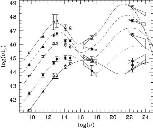
Figure 1: The variation of the average spectral energy distribution of blazars with radio luminosity [9]. The low-energy component, due to synchrotron radiation, peaks in the infrared for “red”, low-energy peaked blazars, and at UV/X-ray energies for “blue”, high-energy peaked blazars. Note how the location of the synchrotron peak varies with luminosity.

The blazar class covers a very wide range in luminosity as well as peak frequency. More luminous objects tend to peak at lower frequencies, but there is a wide scatter in this relation Fossati98 . Historically, optical spectroscopic properties have been used to separate blazars into two divisions: flat-spectrum radio quasars (FSRQ) have strong, broad emission lines, while BL Lacs have very faint or no emission lines. However, this distinction now appears arbitrary, as recent work has shown a continuous distribution of emission line luminosities and equivalent widths ScFa97 .

I will review the surveys which have been used to find blazars as well as their biases, and show how this has produced two populations with somewhat different properties. I will for pedagogical reasons adopt the traditional division between BL Lacs and FSRQ, but I believe that one of the most important tasks the new surveys must undertake is to define new, physically based classes for blazars. I will describe the latest crop of surveys and their findings, and “round up” a herd of objects which should be targets for the new generation of VHE gamma-ray observatories.

II Survey Methods and Biases

Because of their rareness, blazars have an unfortunate history of divisions “invented” because of observed properties or selection methods which may not have any physical basis. The result has been confusion not only over how to define subclasses and their properties, but indeed over the definition of the blazar class itself! The BL Lac/FSRQ division is an example of this phenomenon; another is the definition of “radio-selected” and “X-ray selected” BL Lac classes, based on the survey in which an object was found. Yet several well known objects turn up in both radio and X-ray surveys, for example Mkn 421, Mkn 501 and BL Lac.

Our understanding is helped considerably if we take a step back and try to understand the biases inherent in single-band surveys. The key point (which seems obvious but is in fact surprisingly subtle) is that any survey selects preferentially objects that are bright in the survey band. Thus the overwhelming majority of blazars selected in X-rays peak in the UV or X-rays, while nearly all blazars selected in the radio peak at much lower (IR) energies (Figure 1). The subtlety lies in the fact that these two methods attack opposite ends of parameter space (Figure 2), and do seem to find objects with somewhat different properties (more about this in §III). Thus while inquiries into blazar properties have achieved much by using X-ray and radio selected samples, they have hardly delved into what connects them.

Figure 2: Two views of the radio-optical-X-ray flux parameter space for previous samples of BL Lacs. 1 Jy BL Lacs are shown plotted as triangles, S4 BL Lacs are shown plotted as squares, Slew BL Lacs are shown as pluses, and EMSS BL Lacs are shown as asterisks. Note the large gaps which existed prior to 1995 in our coverage of this parameter space.

Today we speak of “high-energy peaked” and “low-energy peaked” blazars, referring to objects which peak at (respectively) UV/X-ray or infrared energies. The disparity in the peak frequencies indicates significant differences in jet physics. This is expected on theoretical grounds, since the characteristic electron energy for synchrotron emission is directly related to the magnetic field $(\gamma_{peak}\propto\sqrt{\nu_{peak}/B})$. Moreover, the trends we find with luminosity (decreasing $\nu_{peak}$, increasing emission line luminosity) indicate substantially more cooling in more luminous objects.

The location of the synchrotron peak is intimately connected to which kinds of objects are observed to dominate at GeV and TeV gamma-ray energies. At GeV energies, lower-energy peaked, high-luminosity objects dominate, as they have much higher ratios $L_{C}/L_{S}$. These objects, however, do not make electrons with $\gamma\sim 10^{6-7}$, which are required for X-ray synchrotron emission, probably because of increased cooling. Thus at TeV energies, objects which peak in the UV/X-rays (i.e., high-energy peaked or X-ray selected blazars) are all that is seen.

Unfortunately, current surveys do not contain enough information to tell us which kind of blazar (high or low-energy peaked) is more common. This is because current complete samples cover very shallow dynamic ranges (Figure 2). There is a general indication that high-luminosity objects are less common UrPa95 . However, deeper surveys are needed, because finding the absolute number of either kind of object requires correcting current surveys for the objects it does not find – and to do this, we must go deep enough in both radio and X-ray so that radio surveys start detecting significant numbers of high-energy peaked blazars, and vice versa.

III The Properties of Red and Blue Blazars

Over the last decade, many workers have delved into the properties of high-energy peaked and low-energy peaked blazars, by using samples of BL Lacs selected in the radio and X-rays. BL Lacs were used in this work because until very recently there were no FSRQ known to peak at UV/X-ray energies(Perlman98 ; PaGi97 ; PaPe99 ; §IV). These works found significant differences between the properties of blue, high-energy peaked BL Lacs (HBLs) and red, low-energy peaked BL Lacs (LBLs):

• HBLs are less luminous in radio and bolometrically Sambruna96 ; Fossati97 ; Fossati98 .

• HBLs are less core-dominated in the radio than LBLs PeSto93 ; PeSto94 ; L-M93 ; Koll96 ; Rector99 .

• HBLs are less polarized than LBLs, with a smaller duty cycle, and tend to have a preferred position angle of polarization, while LBLs do not Jannuzi93 .

• Occupy a different region of X-ray-optical-radio parameter space (Figure 2), and in fact a unique region of parameter space in X-ray-optical and radio-optical spectral index space (Figure 3, Stocke91 ).

• HBLs tend to have steeper X-ray and optical-X-ray continua than LBLs Perlman96 ; Sambruna96 ; Urry96 ; Lamer97 ; Padovani97 .

• HBLs are distributed differently in space, with more objects or more luminous objects (current samples cannot discriminate between these possibilities) at low redshifts Morris91 ; Wolter94 ; Perlman96 ; Bade98 ; Giommi99 ; Rector99 ; while LBLs are consistent with either a uniform distribution with redshift or more objects at high redshift Stickel91 .

As with their properties, the relationship between HBLs and LBLs has been a subject of active debate in the literature. At first it was thought that they were related through viewing angle (e.g., Ghis93 and refs. therein). This explained many properties in a natural way, for example the differences in polarization behavior and radio core dominance (though see Rector99 for new counter-evidence), as well as the observed difference in space density (which could have been a selection effect, however; see §II). A second model was proposed by Padovani & Giommi GiPa94 ; PaGi95 , under which HBLs and LBLs represent two ends of a continuous distribution of synchrotron peak frequencies. It turns out that both descriptions have problems. Rita Sambruna showed in her thesis Sambruna96 that differences in in viewing angle cannot produce a variation of $10^{4}$ in peak frequency. And while the “different peak frequencies” description is accurate phenomenologically, it cannot by itself explain the differences in radio core-dominance Koll96 ; Stocke96 and polarization PA Stocke96 behavior.

This question is still open, but a modern view is evolving which basically says that both the viewing angle and different spectral energy distributions pictures have a piece of the puzzle. Two competing models now ascribe the HBL-LBL relationship to combinations of luminosity and viewing angle GeoMa98 , or luminosity and peak frequency Ghis98 . Current data cannot distinguish between these models, although further investigation of the polarization differences with larger samples and in multi-wavelength campaigns, offer in my view the best hope for doing so.

IV The New Surveys: Bridging the Gaps

As I discussed in §II, the existing complete samples of blazars suffer from several problems. First of all they are small: typically a few dozen objects at most. There are also various concerns about completeness, particularly at the lowest luminosities (e.g., BroMar93 ; MarBro95 ; MarBro96 ; Perlman96 ; RSP99 ). But the most difficult problems have to do with the small dynamic ranges covered in flux and luminosity (cf. Figure 2).

In this section we review the latest information on existing samples. However, we will concentrate largely on four new surveys which are bridging the gaps in our coverage of parameter space. These surveys are allowing us to for the first time actively pursue the connections between blazar classes and get at the real physics. The most exciting discovery of these surveys is the existence of a large population of high-energy peaked FSRQ. We will reanalyze two existing samples in the light of these findings, and show that their makeup is consistent with the new surveys.

The existing samples of blazars are listed below:

• Einstein Slew Survey Perlman96b ; Perlman99 : $F(X)\gtrsim 10^{-11}{\rm~{}erg~{}cm^{-2}~{}s^{-1}}$, $F(R)>1$ mJy, 50% of the sky. 66 BL Lacs, 19 FSRQ. Includes all known TeV emitters.

• Einstein EMSS Stocke91 ; Morris91 ; Rector99 ; Perlman99 : $F(X)>2\times 10^{-13}{\rm~{}erg~{}cm^{-2}~{}s^{-1}}$, $F(R)>1$ mJy, 2% of the sky. 43 BL Lacs, 16 FSRQ.

• 1 Jy Stickel91 ; Stickel93 ; Stickel94 : $F(R)>1$ Jy, 60% of sky. 37 BL Lacs, 222 FSRQ, but not completely identified.

• S5 StiKu96 : $F(R)>250$ mJy, $\delta>70^{\circ}$. 11 BL Lacs, 20 FSRQ, but not completely identified.

• S4 StiKu94 : $F(R)>500$ mJy, $35^{\circ}<\delta<70^{\circ}$. 7 BL Lac, 56 FSRQ, but not completely identified.

Figure 3: X-ray-optical and Optical-Radio Spectral indices of FSRQ and BL Lacs discovered in radio and X-ray surveys[34,35]. Note the vastly different ranges of parameter spaces covered by historical radio surveys (1 Jy: open squares) compared to X-ray surveys (DXRBS and RGB: see §4). Prior to 1996, in fact, the parameter space covered by X-ray and radio techniques was almost completely disjoint, as shown in Figure 2.

Figure 4: X-ray and Radio luminosities for FSRQs[34,35]. Note that high-energy peaked FSRQs (right of the dashed line) are less luminous in the radio (for the same X-ray luminosity). DXRBS and RGB sample unexplored regions of parameter space, containing objects $\sim 20\times$ less luminous than previous surveys.

Four new surveys are in progress, filling vast new regions of parameter space (Figures 3,4). These surveys are listed in Table 1.

Table 1: New Surveys for Blazars

					Flux Limit
Survey	BL	$z<0.1$	FSRQ	$z<0.1$	F(0.1-2 keV)	F(R)	Types of Objects
	Lacs				${\rm~{}erg~{}cm^{-2}~{}s^{-1}}$	mJy
DXRBSPerlman98 ; Landt99 ; PaPe99	40	5	218	0	$10^{-14}$	25-50	most LBL/intermediate
RGB Brink97 ; L-M98 ; L-M99	127	14	252	9	$10^{-12}$	25	most HBL/intermediate
NVSS-RASSGiommi99	58	1	?	?	$10^{-12}$	3.5	all HBL
REXCaccia99	?	?	?	?	$10^{-14}$	3	mostly HBL

The depth and size of these new surveys has allowed them to probe much deeper into the luminosity function of blazars than ever before. Close examination of Figures 3 and 4, and comparison with Figure 2 reveals two key discoveries. First of all, the number of FSRQ with radio luminosity $L_{R}<10^{26.5}{\rm~{}W~{}Hz^{-1}}$ has increased nearly ten-fold, and for the first time luminosities below $10^{25.5}{\rm~{}W~{}Hz^{-1}}$ are being reached (an equally large expansion of the number of low luminosity BL Lacs is also taking place). This is important because the knee in the radio luminosity function of FSRQ is located at or near $10^{26.5}{\rm~{}W~{}Hz^{-1}}$, and the location of the knee and the shape of the luminosity function below the knee are very poorly constrained due to the paucity of low luminosity objects in current samples. The second, equally important discovery, is that because these surveys have plugged the holes in our coverage of X-ray-optical-radio parameter space, they have revealed large numbers of blazars in regions of parameter space where previously very few were known Perlman98 ; L-M98 ; PaPe99 ; L-M99 . These objects fall into two categories: intermediate BL Lacs, which have peak energies $\sim 1-10$ eV, and X-ray bright FSRQ, which some authors had predicted did not exist due to the observed continuity in broadband spectral properties between the blazars known in complete samples in 1996 Sambruna96 . These two discoveries are in fact not completely independent of one another, because the lowest luminosities are dominated by high-energy peaked objects (Figure 4).

The X-ray bright FSRQ are in fact particularly important for our knowledge of the class, because they overlap significantly in radio and bolometric luminosities with the low-energy peaked BL Lacs. Investigations into their properties and comparisons with previously known FSRQ hold the promise of truly understanding the connections between different classes of blazars. A similar thing can be said for the intermediate BL Lacs; but since the range of parameter space opened up is larger for the emission line objects and the potential impact on VHE gamma-ray astronomy from them is greater, I will concentrate on them in this paper.

The DXRBS collaboration has begun an investigation into the properties of X-ray bright FSRQ. We find that these objects differ in important ways from their lower-energy peaked cousins (in most cases paralleling radio/X-ray selected BL Lac differences). These differences (Figure 5) include ROSAT spectra that are steeper than known FSRQ PaPe99 ; Sambruna97 , and SEDs that appear to peak in the UV/X-rays, based on ROSAT, optical and radio catalog data PaPe99 . They also overlap significantly with HBL BL Lacs on the $(\alpha_{ro},\alpha_{ox})$ plane (Figure 3). However, observations of several of these objects at harder X-ray energies with ASCA and SAX have revealed that most (but not all) have rather flat spectra, more similar to other FSRQ than HBL BL Lacs (Sambruna99 ; Costa99 , although note that the selection criteria were different).

Figure 5: At left, the radio to X-ray SED of two high-energy peaked FSRQ [35]. The data clearly point to a spectral peak in the UV/X-ray, similar to HBL BL Lacs. At right, ROSAT spectral indices of DXRBS FSRQ with radio-to-X-ray spectral indices above and below 0.78 [35], which is equivalent to the diagonal line at log $L_{x}/L_{R}=10^{-6}$ on Figure 4. The spectra of the X-ray brighter objects are steeper than those of more radio-loud “traditional” FSRQ.

This last observation is a fly in the ointment, because the most natural explanation of the radio to X-ray SEDs derived from survey data is synchrotron radiation from a single population of electrons, as with HBL BL Lacs. If indeed this paradigm holds, one would expect steeper hard X-ray spectra, dominated by the steep tail of the particle distribution. The observation that many of these objects appear to have flat hard X-ray spectra is difficult to explain in this context (note that the curvature is in the opposite sense for “blue bump” emission, however). There are several possibilities. For example, if Compton cooling is stronger in these objects (due to higher electron density, for example) than HBL BL Lacs, Comptonization could begin to dominate the energy budget at energies of a few keV instead of tens to hundreds of keV as it does in the HBL BL Lacs. It is also possible that there might be some Compton reflected emission from the accretion disk in the hard X-rays, as there is for Seyfert galaxies (e.g., Grandi98 ). However, no spectral curvature is seen at a few keV Costa99 ; Sambruna99 ; nor do we see a strong Fe K$\alpha$ line from the inner reaches of the accretion disk, as is seen in Seyferts. There is also a question of selection: Padovani & Giommi GiPa94 ; PaGi95 showed that (assuming a roughly parabolic SED), a hypothetical object moves diagonally down on the ($\alpha_{ox},\alpha_{ro}$) plane (roughly along the locus of the 1 Jy sample) until its peak reaches the optical, after which it begins to move horizontally to the left (roughly along the locus of the X-ray selected surveys). Thus one may need to make two cuts (in $\alpha_{ro}$ and $\alpha_{rx}$, as below) rather than one in order to select high-energy peaked objects.

If indeed the radio to X-ray continuum in high-energy peaked FSRQ is produced by synchrotron radiation, one might expect that Comptonized emission would peak at around 1 TeV (similar to HBL BL Lacs), so that these objects should be targets for new TeV observatories. However, this assumes that the balance of mechanisms in Compton cooling is not too different in these objects than it is in HBL BL Lacs.

To produce a list of TeV candidates, I analyzed the DXRBS and RGB samples, as well as existing surveys, which previously had unknown numbers of FSRQ. I found significant numbers of FSRQ in both the EMSS (16) and Slew (19); About 30% of these appear to be high-energy peaking objects (Perlman99 ; 7/16 in the EMSS and 4/19 in the Slew), consistent with the DXRBS and RGB results PaPe99 . I have selected from these surveys $z<0.1$ objects with $\alpha_{ro}<0.6$ and $\alpha_{rx}<0.78$ and F(X)$>10^{-12}{\rm~{}erg~{}cm^{-2}~{}s^{-1}}$. The result is shown in Table 2.

Table 2: Suggested Candidates for TeV Emission

Name	RA	Dec	F(0.3–3.5 keV)PaGi97	$F(R)$	$z$	ID
	(J2000)		$10^{-12}{\rm~{}erg~{}cm^{-2}~{}s^{-1}}$	mJy
1ES0033+595	00 35 52.7	+59 50 04	75.1	66	0.086	BL Lac
RGB0110+418	01 10 04.8	+41 49 50	2.5	40	0.096	BL Lac
RGB0152+017	01 52 39.7	+01 47 18	5.0b	51	0.080	BL Lac
RGB0153+712	01 53 25.9	+71 15 07	3.1b	643	0.022	BL Lac
RGB0214+517	02 14 17.9	+51 44 52	13.0b	291	0.049	BL Lac
RGB0314+247	03 14 02.7	+24 44 31	2.1b	6	0.054	BL Lac
1ES0548–322	05 50 41.9	$-$32 16 11	44.1	170	0.069	BL Lac
RGB0656+426	06 56 10.7	+42 37 02	3.9b	480	0.059	BL Lac
Mkn 180	11 36 26.4	+70 09 28	7.1	94	0.046	BL Lac
RGB1532+302	15 32 02.2	+30 16 28	5.9b	42	0.064	BL Lac
RGBJ1610+671	16 10 02.6	+67 10 29	4.8b	36	0.067	BL Lac
1ES1727+502	17 28 18.5	+50 13 11	13.7	159	0.055	BL Lac
1ES1741+196	17 43 57.5	+19 35 10	24.6	223	0.083	BL Lac
1ES1959+650	19 59 59.9	+65 08 55	83.4	252	0.048	BL Lac
PKS2005–489	20 09 25.3	$-$48 49 53	16.1	1192	0.071	BL Lac
1ES2321+419	23 23 52.0	+42 11 00	2.2	19	0.059	BL Lac
RGB 2322+346	23 22 44.0	+34 36 14	2.2b	78	0.098	BL Lac
III Zw 2	00 10 31.0	+10 58 28	4.8	420	0.090	FSRQ
B2 0138+398	01 41 57.8	+39 23 30	1.1b	115	0.080	FSRQ
B2 0321+33	03 24 41.2	+34 10 45	6.6	364	0.062	FSRQ
RGB1413+436	14 13 43.7	+43 39 45	4.5b	39	0.090	FSRQ
PG 2209+184	22 11 53.7	+ 18 41 51	8.4	134	0.070	FSRQ

Importantly, lists such as Table 2 should not serve as a be-all and end-all for future TeV surveys. This is particularly true for southern hemisphere observers, since most blazar surveys unfortunately cover very little of the southern sky! It is very important that large angle TeV surveys be carried out in the near future, and I am encouraged to see that one is now being plannedDingus99 . It has become a truism that every time a large-area survey is done in a new waveband, some completely unexpected discovery is made. It is also equally true that without large-area surveys, it is not possible to correctly derive physics for an entire class. An example of this comes from comparing the ratio of GeV to radio emission typical for EGRET detected blazars ($\sim 700$) with that required of all blazars in order to produce the diffuse GeV background ($\sim 70$; KaPe97 ; SteSa96 ). If we based all our modeling of how the GeV continuum of blazars is produced upon the assumption that nature only makes blazars with GeV/radio ratios in the hundreds, our model would not be accurate for the vast majority of sources. The same holds in the TeVUrry99 .

V Conclusions

It is safe to say that there are many key open questions in blazar research. Future surveys will be crucial in addressing many of these. Here are a few examples:

• What is the nature of the HBL-LBL relationship (in both BL Lacs and FSRQ), and the BL Lac-FSRQ relationship? These questions can only be addressed properly when radio selected samples have large numbers of HBL type objects, and X-ray selected samples have large numbers of LBL type objects. Gamma-ray surveys can also help here: each model for the production of gamma-rays has a different dependence on viewing angle and Lorentz $\Gamma$ Boe99 ; Rach99 ; Mast99 .

• What constrains emission line luminosity and what role does the emission line luminosity play in gamma-ray production in various types of blazars? One prerequisite for answering this question now exists: large surveys which contain blazars of all X-ray/radio continuum and emission line luminosity classes. But the other does not: a gamma-ray database that includes variability information on statistically significant numbers of objects at all luminosities.

• What are the gamma-ray spectral energy distributions of all blazars? The prerequisite for answering this survey is gamma-ray surveys in the MeV, GeV and TeV ranges, which are deep enough to contain statistically significant numbers of blazars of all continuum and emission line luminosity classes.

• Are blazars (whether aligned or misaligned) really the only extragalactic objects which produce detectable quantities of gamma-rays with energies greater than $\sim 10$ MeV? This question is intimately related to the issue of what produces the gamma-ray backgroundKaPe97 .

These questions, and the new issues they raise, are intimately connected with, and equally as important, as those that will be addressed (and raised) in multiwavelength campaigns and modelling efforts.

This paper summarizes work I have done in collaboration with several other scientists. I would particularly like to acknowledge my DXRBS collaborators, Paolo Padovani, Paolo Giommi, Hermine Landt and Rita Sambruna.

References

- (1) Bade, N., Beckmann, V., Douglas, N. G., Barthel, P. D., Engels, D., Cordis, L., Nass, P., & Voges, W., 1998, A & A 334, 459.
- (2) Böttcher, M., 1999, these proceedings.
- (3) Brinkmann, W., Siebert, J., Feigelson, E. D., Kollgaard, R. I., Laurent-Muehleisen, S. A., Reich, W., Fuerst, E., Reich, P., Voges, W., Trümper, J., McMahon, R., 1997, A & A 323, 739.
- (4) Browne, I. W. A., & Marchã, M. J. M., 1993, MNRAS 261, 795.
- (5) Caccianiga, A., Maccacaro, T., Wolter, A., Della Ceca, R., Gioia, I. M., 1999, ApJ 513, 51.
- (6) Costamante,L., Padovani, P., Perlman, E., Giommi, P., 1999, in preparation.
- (7) Dingus, B., these proceedings.
- (8) Fossati, G., Celotti, A., Ghisellini, G., & Maraschi, L., 1997, MNRAS 289, 136.
- (9) Fossati, G., Maraschi, L., Celotti, A., Comastri, A., & Ghisellini, G., 1998, MNRAS 299, 433.
- (10) Georganopoulos, M., & Marscher, A. P., 1998, ApJ 506, 621.
- (11) Ghisellini, G., Padovani, P., Celotti, A., & Maraschi, L., 1993, ApJ 407, 65.
- (12) Ghisellini, G., Celotti, A., Fossati, G., Maraschi, L., & Comastri, A., 1998, MNRAS 301, 451.
- (13) Giommi, P., Menna, M. T., & Padovani, P., in preparation.
- (14) Giommi, P., Menna, M. T., & Padovani, P., 1999, MNRAS in press (astro-ph/9907014).
- (15) Giommi, P., & Padovani, P., 1994 MNRAS 268, L51.
- (16) Giommi, P., Tagliaferri, G., Bueurmann, K., Branduardi-Raymont, G., Brissenden, R., Graser, U., Mason, K. O., Mittaz, J. D. P., Murdin, P., Pooley, G., Thomas, H.-C., & Tuohy, I., 1991, ApJ 378, 77.
- (17) Grandi, P., Haardt, F., Ghisellini, G., Grove, E. J., Maraschi, L., & Urry, C. M., 1998, ApJ 498, 220.
- (18) Jannuzi, B. T., Smith, P. S., & Elston, R., 1993, ApJ 428, 130.
- (19) Kazanas, D., & Perlman, E., 1997, ApJ 476, 7.
- (20) Kollgaard, R. I., 1994, Vist. Astron 38, 29.
- (21) Kollgaard, R. I., Palma, C., Laurent-Muehleisen, S. A., & Feigelson, E. D., 1996, ApJ 465, 115.
- (22) Lamer, G., Brunner, H., & Staubert, R., 1996, A & A 311, 384.
- (23) Landt, H., Perlman, E. S., Padovani, P., & Giommi, P., 1999, MNRAS, submitted.
- (24) Laurent-Muehleisen, S. A., Kollgaard, R. I., Ciardullo, R., Feigelson, E. D., Brinkmann, W., & Siebert, J., 1998, ApJS 118, 127.
- (25) Laurent-Muehleisen, S. A., Kollgaard, R. I., Feigelson, E. D., Brinkmann, W., & Siebert, J., 1999, ApJ in press (astro-ph/9905133).
- (26) Laurent-Muehleisen, S. A., Kollgaard, R. I., Moellenbrock, G. A., & Feigelson, E. D., 1993, AJ 106, 875.
- (27) Marchã, M. J. M., Browne, I. W. A., Impey, C. D., & Smith, P. S. 1996, MNRAS 281, 425.
- (28) Marchã, M. J. M., & Browne, I. W. A., 1996, MNRAS 279, 72.
- (29) Mastichiadis, A., 1999, these proceedings.
- (30) Morris, S. L., Stocke, J. T., Gioia, I. M., Schild, R. E., Wolter, A., Maccacaro, T., & Della Ceca, R., 1991, ApJ 380, 49.
- (31) Padovani, P., & Giommi, P., 1995, ApJ 444, 567.
- (32) Padovani, P., Giommi, P., & Fiore, F., 1997, in Mem. Astron. Soc. Italia 68, 147.
- (33) Padovani, P., Giommi, P., & Fiore, F., 1997 MNRAS 284, 569.
- (34) Padovani, P., Perlman, E., Landt, H., Sambruna, R., Giommi, P., 1999, MNRAS, submitted.
- (35) Perlman, E. S., Padovani, P., Giommi, P., Sambruna, R., Jones, L. R., Tzioumis, A., & Reynolds, J., 1998, AJ 115, 1253.
- (36) Perlman, E. S., Schachter, J. F., & Stocke, J. T., 1999, in preparation.
- (37) Perlman, E. S., & Stocke, J. T., 1993, ApJ 406, 430.
- (38) Perlman, E. S., & Stocke, J. T., 1994, AJ 108, 56.
- (39) Perlman, E. S., et al., 1996, ApJS 104, 251.
- (40) Perlman, E. S., Stocke, J. T., Wang, Q. D., & Morris, S. L., 1996, ApJ 456, 451.
- (41) Rachen, J., 1999, these proceedings.
- (42) Rector, T. A., Stocke, J. T., & Perlman, E. S., 1999, ApJ 516, 145.
- (43) Rector, T. A., Stocke, J. T., Perlman, E. S., & Morris, S. L., 1999, ApJ submitted.
- (44) Sambruna, R. M., these proceedings.
- (45) Sambruna, R. M., 1997, ApJ 487, 536.
- (46) Sambruna, R. M., Maraschi, L., & Urry, C. M., 1996, ApJ 463, 444.
- (47) Scarpa, R., & Falomo, R., 1997 A & A 325, 109.
- (48) Stecker, F. W., & Salamon, M. H., 1996, ApJ 464, 600.
- (49) Stickel, M., Fried, J. W., & Kühr, H., 1993, A & A S 268, 53.
- (50) Stickel, M., Fried, J. W., Kühr, H., Padovani, P., & Urry, C. M., 1991, ApJ 374, 431.
- (51) Stickel, M., Meisenheimer, K., & Kühr, H., 1994, A & A S 105, 211.
- (52) Stickel, M., & Kühr, H., 1994a, A & A S 103, 349.
- (53) Stickel, M., & Kühr, H., 1994a, A & A S 115, 1.
- (54) Stocke, J. T., Morris, S. L., Gioia, I. M., Maccacaro, T., Schild, R., Wolter, A., Fleming, T. A., & Henry, J. P., 1991 ApJS 76, 813.
- (55) Stocke, J. T., 1996, in Extragalactic Radio Sources, IAU 175, ed. R. D. Ekers, C. Fanti, and L. Padrielli (Kluwer: Dordrecht), p. 385
- (56) Urry, C. M., & Padovani, P., 1995, PASP 107, 803.
- (57) Urry, C. M., Sambruna, R. M.,Worrall, D. M., Kollgaard, R. I., Feigelson, E. D., Perlman, E. S., Stocke, J. T., 1996, ApJ 463, 424.
- (58) Urry, C. M., 1999, Astroparticle Physics 11, 159.
- (59) Wolter, A., Caccianiga, A., Della Ceca, R., & Maccacaro, T., 1994, ApJ 433, 29.