Abstract

We describe the calibration, measurements and data reduction, of the dark current of the ISOCAM/LW detector. We point-out the existence of two significant drifts of the LW dark-current, one throughout the ISO mission, on a timescale of days, another within each single revolution, on a timescale of hours. We also show the existence of a dependence of the dark current on the temperature of the ISOCAM detector.

By characterizing all these effects through polynomial fittings, we build a model for the LW calibration dark, that depends on the epoch of observation (parametrized with the revolution number and the time elapsed in that given revolution since the activation) and on the temperature of the ISOCAM detector. The model parameters are tuned for each of ISOCAM/LW pixel.

We show that the modelling is very effective in taking into account the dark-current variations and allows a much cleaner dark subtraction than using a brute average of several calibration dark images.

The residuals of the LW model-dark subtraction are, on average, similar to the pre-launch expectation.

1 Introduction

In this document we describe the calibration of the dark current in the ISOCAM/LW detector.

The term “dark current” will be used throughout this paper to indicate the level of the signal measured when the detector is in darkness, i.e. when no external flux reaches the detector. Strictly speaking, this is not a current, but an electronic reference level including both real dark current and electrical offsets. For the LW detector, this signal is due to thermal charge generation in the photoconductors and charge leakage generated during the commutation of the reset transistor (see the “Observer’s Manual for ISOCAM”). A typical example of the pattern measured on the LW detector in darkness is shown in Fig. 1 (for an integration time – T_int hereafter – of 2 sec). The LW dark frame shows a line pattern with a clear separation between odd and even lines.

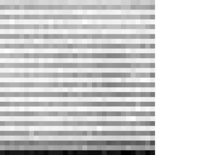
Figure 1.  : An example of the LW dark frame, measured at T_int =2 sec. Note the very evident line pattern.

The output of the pixels of the detector at dark is given in the standard units of all observations done with the ISOCAM/LW detector, i.e. the Analog-to-Digital Units (ADU, hereafter). For a gain factor $\times 2$, one ADU corresponds to 120 electrons above a given electrical offset (see the “Observer’s Manual for ISOCAM”). Since the dark measurements are sometimes done with a gain factor $\times 1$, and sometimes with a gain factor $\times 2$, for the sake of simplicity in this document we scaled all units by the gain factor – i.e. we use ”ADU” to mean “Analog-to-Digital Units scaled by the gain factor”.

The ISOCAM dark measurements have been done at several integration times, because the dark current (i.e. the measured output per pixel of the detector in the darkness) has no simple linear dependence on the integration time. The pixel values can therefore be expressed in terms of the ADU received per given integration time, or in terms of the ADU received per second, by rescaling the measured output value by the integration time. Hereafter, we will express the dark current values either in ADU or in ADU/s, and specify the integration time used in order to allow translation from one unit to another.

In summary, the observed value of the dark current, in ADU, on a given pixel, is given by:

$$D_{O}=(N_{e^{-}}-offset)/(gain\times 60)$$ (1)

where $N_{e^{-}}$ is the number of electrons on the capacity of the detector.

During the ISO mission it was shown that the LW dark-current is drifting both on a timescale of hours within a given revolution, and on a timescale of days throughout the mission. Hereafter we will refer to these drifts as the short-term and long-term trends of the dark current.

The dark currents have been calibrated with four different kinds of observations:

• Darks measured during calibration-dedicated revolutions, i.e. those that are specifically dedicated to calibration observations (typically, one per week); we call these measurements the calibration darks.

• Darks measured during the handover period, i.e. when the satellite tracking switches from one of the two antennae (VILSPA or Goldstone) to the other (this time typically lasts 15–30 min every revolution); we call these measurements the handover darks.

• Darks measured during the deactivation period (lasting typically 1 hour every revolution) i.e. when ISO enters the Earth radiation belts and scientific observations are no longer possible because of the high rate of glitch impacts, just before all instruments have to be switched off; we call these measurements the deactivation darks.

• Darks measured in the ISOCAM parallel mode of observation, i.e. taking advantage of the part of telemetry (1/12) that is reserved to ISOCAM when other ISO instruments are observing in prime mode; we call these measurements the parallel-mode darks.

The four types of dark measurements have different goals. The calibration darks  are long measurements done throughout the mission to constrain the pattern of the dark frame, i.e. the dark current variation from one pixel to another. The calibration darks  are measured at regularly spaced time intervals, typically one measure at all T_int every month. These time intervals are not so dense as to allow a very clean characterization of the long-term drifts of the dark currents. On the other hand, specific repeated observations of the dark current throughout the same revolution allow to constrain the short-term drift (as we will see in § 5).

A proper characterization of the long-term drifts is provided by the handover darks, which are shorter (and therefore noisier) measurements done at every revolution, throughout the whole ISO mission, and more or less at the same time after the activation of the instrument. Unfortunately, the limited time available during the handover sequence imposed severe constraints on the measurements, and it was decided to monitor only two T_int (2 and 5 sec) LW darks during handover. Starting with the revolution 764 (december 1997), the handover sequence of dark measurements has been changed in order to monitor also the 0.28 and 10 sec LW darks, as it was understood that the long-term drift was important, and it was necessary to check that the drift was the same (or at least similar) at different T_int (see § 3). Since revolution 764, the even days were dedicated to the measurements of darks at T_int =0.28 and 10 sec, and the odd days to the darks at T_int =2 and 10 sec. The dark at T_int =20 sec was not covered, because of time limitation (notice that ISOCAM observations at T_int =20 sec are strongly affected from glitches, so that this T_int was very seldom used by observers).

The deactivation darks  include LW dark measurements at T_int =2 and 5 sec. One could think that the deactivation darks  provide a monitoring of the long-term trend of the dark currents. Unfortunately, these deactivation darks  are strongly affected by the so-called space weather, i.e. particles in the Earth environment (for further details, see Gallais & Boulade 1998).

Most of the measurements of parallel-mode darks  were done in the last seven months of the ISO mission. Based on the repeated measurements of calibration darks  in a single revolution, the short-term drift of the LW dark current was discovered. As a consequence, a denser time monitoring of the LW dark current was required. In order to have more measurements, and to avoid using too much calibration time, it was decided to have dark measurements with ISOCAM in the parallel mode. Even with the reduced telemetry rate available, these measurements have since proven to be extremely useful to constrain the dark drifts within single revolutions. These measurements have been done at all LW T_int , with the exception of T_int =0.28 sec, unfeasible because of a software limitation in the total number of frames that can be accumulated on-board. However, several calibration darks  have been measured at this particular T_int to fill this gap.

2 Dark data-reduction

The data-reduction of dark measurements consists in deglitching, and averaging (or taking the median) of the stabilized frames.

2.1 Deglitching

Deglitching is always a very complicated operation for ISOCAM observations. Several deglitching methods are used for the dark measurements, but typically the most used are TCOR, TEMP, and MM, all methods implemented in the CAM Interactive Analysis, CIA software package (Ott et al. 1996, Delaney 1998).

The TEMP method of deglitching has been used in the early times of the ISO mission for the data-reduction of calibration darks, while the MM method has been used in the most recent times. The two methods provide essentially identical results. More specifically, we can quantify the difference as follows. After deglitching the same set of dark frames with the two methods, we subtracted one of the resulting dark image from the other; the residuals of this subtraction quantify the importance of using two different methods of deglitching. The average residual difference (over all pixels) is less than 0.005 ADU, with a root-mean-square (RMS hereafter) of 0.04 ADU and the maximum difference is 0.16 ADU.

On the other hand, the TCOR method has been used for the deglitching of handover darks  (Gallais & Boulade 1998), and it does give slightly different results from the previous two methods. The final dark images as obtained from the same data-set but with either the TCOR deglitching method, or the MM one, differ by, on average, 0.07 ADU, with an RMS of 0.12 and a peak difference of 0.34 ADU. These differences arise from the lower deglitching efficiency of the TCOR method. Since faint glitches are not detected by the TCOR method, yet they are detected by the TEMP or the MM ones, and glitches always contribute a spurious positive signal when the detector is at dark, the resulting dark level after deglitching is always sistematically higher when the TCOR method is used.

Luckily, the handover darks  are only used for establishing a linear trend over long timescales (see § 3) and the good statistics (handover darks  are measured every day) compensates for the additional noise induced by an imperfect deglitching. The overall positive offset of the mean level of handover darks  is not a problem, as it can be corrected using the calibration darks  and/or the parallel-mode darks  (see § 5).

2.2 Stabilization

As the ISOCAM detector has a slow response to flux variations, it takes some time for an ISOCAM pixel to level off to the dark level from a pre-existing condition of illumination. Often, even in very long dark measurements, stabilization is not achieved. As an example of different behaviours, we show in Fig. 2 the mean dark level vs. the frame number in four calibration darks  at T_int =2 sec. After an initial increase, due to the change of integration time from a previous dark measurement, the dark level slowly decreases to its stabilized value. It is clear that only the last frames must be used to form the final (stabilized) image.

As an additional example, we show in Fig. 3 the handover darks  measured at 2 and 5 sec T_int , i.e. the mean current level measured in the ISOCAM/LW detector vs. the frame number. In the T_int =2 sec dark measurement, one can see the initial decrease due to the fact that ISOCAM was open before the dark measurement; in the T_int =5 sec dark measurement, one can see the current change due to the change in T_int , followed by another long period of stabilization to the level of the dark current at T_int =5 sec.

Figure 2.  : The mean dark current level vs. frame number in four calibration darks  measurements at T_int =2 sec. Note the slow stabilization drifts.

Figure 3.  : The mean dark current level vs. frame number in two handover darks  measurements at T_int =2 and 5 sec. Note the slow stabilization drifts.

Figure 4.  : The mean dark current level vs. frame number in four parallel-mode darks  measurements at T_int =5 sec. Note the stabilization drift to the darkness level, after the illumination of the detector during the handover (bottom-left panel).

Finally, we give in Fig. 4 four examples of parallel-mode darks. As before, we plot the mean current level vs. the frame number to show the stabilization trend. Generally, the fact that the ISOCAM detector is kept in the same dark configuration during the whole revolution (except for the handover interval) means that stabilization should not be a problem here. However, after handover there is a stabilization drift (this is shown in the lower-left panel of Fig. 4), and additional drifts (of much lower importance, though) arise because of the change in the ISOCAM detector temperature, which is affected by the operations of other ISO instruments (see § 4).

The criteria for choosing the stabilized frames may be slightly different for the three kinds of measurements. In particular, the choice of the stabilized frames of the calibration darks  cannot be blind, as these measurements are not always done in the same conditions of previous illumination of the ISOCAM detector (e.g., the dark measurement could be done after the observation of a calibrating star, or after a parallel mode configuration); depending on what was the previous ISOCAM target, the stabilization trend can be quite different. On the other hand, parallel-mode darks  are always very close to stabilization, so that, after excluding the frames measured just after the handover, all frames can be used to build the dark image, by taking their median. Finally, since the measurements of handover darks  are always done in the same way, the data-reduction procedure is automatic, and only the last 10 frames are averaged to give the final dark image (see Gallais & Boulade 1998). This choice can produce a different mean dark current level for handover darks  as compared to calibration darks  and parallel-mode darks. However, this offset can be (and is) corrected (see § 5).

3 Long-term drift

The handover darks  provide an excellent constraint on the long-term drift of the LW dark current. The mean value of the T_int =2 and 5 sec handover darks  are shown in Fig. 5 and Fig. 6, respectively, from revolution 150 to 829 (handover darks  started to be measured routinely since revolution 150). There is a clear decreasing trend of the dark current, approximately linear with the revolution number. However, the trend is not the same over the whole array, as can be seen in the figures, where the mean values of the odd- and even-line pixels are shown separately. A proper characterization of this trend must therefore take into account individual pixels.

Figure 5.  : The mean values of the odd and even line pixel dark-currents as measured during the handover, vs. the revolution number, at T_int =2 sec.

Figure 6.  : The mean values of the odd and even line pixel dark-currents as measured during the handover, vs. the revolution number, at T_int =5 sec.

For each pixel, we made a linear fit of the dark current drift with revolution. The fitted values of the intercepts define a “zero-revolution” dark frame which we show in Fig. 7. The histograms of the individual pixel long-term drift slopes are shown in Fig. 8 and Fig. 9. It can be seen that the drift is (on average) more negative for even-line pixels than for odd-line pixels, for both T_int , and ranges from $\sim-0.2$ ADU/s, per 100 revolutions to $\sim 0.00$. In order to understand how much of the difference among the individual pixel gradients is real, and how much is due to fitting uncertainties, we repeated the regression analysis separately for two subsamples of equal sizes extracted from the whole sample (i.e. by selecting only odd number revolutions in one subsample, and even number revolutions in another). We found that the average uncertainty on the individual pixel gradients is only $\sim 0.004$ ADU/s per 100 revolutions, much smaller than the pixel-to-pixel variations, which then must be real. As a consequence, applying the same drift correction to all pixels cannot work.

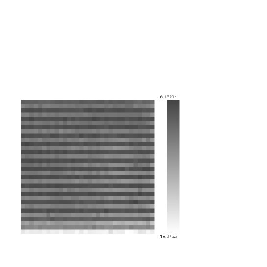
Figure 7.  : The “zero-revolution” dark frame as obtained from the intercepts of the linear fits to each pixel long-term drift, at T_int =2 sec. The grey scale, on the right side, is in ADU/s.

Figure 8.  : The distribution of the long-term drift slopes, in ADU/s/rev, of the individual pixel dark-currents, at T_int =2 sec, obtained by a straight line fitting of the observed value of the dark current of each pixel vs. revolution number.

Figure 9.  : The distribution of the long-term drift slopes, in ADU/s/rev, of the individual pixel dark-currents, at T_int =5 sec, obtained by a straight line fitting of the observed value of the dark current of each pixel vs. revolution number.

The accuracy of this linear-fit characterization of the dark long-term drift can be estimated by computing the RMS variation of the dark current values of all pixels through the mission. The average per-pixel RMS of all handover darks  is $\simeq 0.5$ ADU for both T_int , if we do not apply any correction for the long-term drift. After subtracting from the observed dark current values the fitted ones, the average per-pixel RMS of all handover darks  is reduced to $\simeq 0.25$ ADU.

Other T_int ’s are not well covered in the handover measurements. In particular, the handover measurements at T_int =0.28 and 10 sec started in revolution 764, i.e. only 4 months before the end of the ISO mission. This time coverage is too limited to allow a proper characterization of the trend throughout the whole ISO mission. The situation concerning the T_int =20 sec LW darks is even worse, no measurement being done in handover for this integration time. However, it was possible to make use of the available calibration darks  and handover darks  to constrain the global trend, by properly scaling the linear-fits made on the 2 and 5 sec measurements of handover darks.

We first checked that there was a global consistency among the long-term trends of the handover darks  measured at T_int =2 and 5 sec. Indeed we found that by applying a suitable scaling factor one could deduce the trend at one T_int from the other. Then we checked that the 2 sec long-term trend was consistent with the available data for calibration darks  at T_int =0.28 sec, and, correspondingly, that the 5 sec long-term trend was consistent with the available data for handover darks  and calibration darks  at T_int =10 and 20 sec. A global consistency was found. The scaling was then computed per pixel by averaging a set of dark measurements done at different T_int ’s, during the same epoch of the ISO mission. Specifically, the dark currents at 0.28 sec and 10 sec were computed by averaging the handover measurements of revolutions 764 to 828. In order to obtain the scaling factors, they were divided by the dark currents at 2 sec and, respectively, 5 sec, computed by averaging the handover measurements of revolutions 765 to 829. The lack of handover measurements for the T_int =20 sec dark made this approach impossible, so we simply used a global average of all available measurements to perform the scaling.

The value of the dark current corrected for this long-term drift, $D_{R}$, is obtained from the observed value through the relation:

$$D_{R}=D_{O}-(r_{0}+r_{1}\times rev)$$ (2)

where $D_{O}$ is the observed value of the dark current, in ADU, $rev$ is the revolution number, and $r_{0}$ and $r_{1}$ are the intercept (in ADU) and slope (in ADU/rev) obtained from the linear fit to the long-term trend. The model parameters are different for different pixels and different T_int . In Table 1 we list the average values of these parameters, $<r_{0}>$ (in ADU) and $<r_{1}>$ (in ADU/rev), separately for odd- and even-line pixels, at all T_int .

TABLE 1.  : Results of the linear fits to the long-term trends

 T_int Odd-line pixels Even-line pixels Odd-line pixels Even-line pixels mean intercept mean intercept mean slope mean slope (seconds) $<r_{0}>$ (ADU) $<r_{0}>$ (ADU) $<r_{1}>$ (ADU/rev) $<r_{1}>$ (ADU/rev)  0.28 -7.8 -12.8 -0.0004 -0.0015 2 -14.8 -21.0 -0.0008 -0.0025 5 -17.4 -23.4 -0.0016 -0.0032 10 -19.3 -25.5 -0.0017 -0.0033 20 -20.2 -26.8 -0.0020 -0.0036  

4 The temperature dependence

Once the dark measurements are corrected for the revolution drift, it is possible to show the existence of a relation between the mean dark current and the temperature of the ISOCAM detector. This trend is shown in Fig. 10 for the T_int =0.28 sec calibration darks, after correction for the long-term drift. At the current status of understanding, we can assume that the trend is the same for all pixels and all T_int ’s. The dark current corrected for this temperature dependence, $D_{R,T}$, is obtained through the following relation:

$$D_{R,T}=D_{R}-66.119+17.467\times T$$ (3)

where $T$ is the temperature in K, and $D_{R}$ is the value of the dark current, in ADU, corrected for the long-term drift (see § 3).

Figure 10.  : The correlation between the long-term drift-corrected mean value of the LW dark current at T_int =0.28 sec, as observed in several calibration revolutions, and the ISOCAM detector temperature, in K.

5 Short-term drifts

The short-term drift of the dark current, repeating at each revolution, from the activation of the instrument to its deactivation, was first discovered in the calibration darks. At variance with the handover darks, the calibration darks  are not done at approximately the same time within a revolution. In some cases, several measurements were done during the same revolution at different times. It is then possible to look for the existence of a drift of the dark current with the time elapsed since the activation of the ISOCAM instrument in any revolution (the “time since activation”, tsa hereafter).

Figure 11.  : The mean value of the LW detector dark-current, measured at T_int =0.28 sec in several calibration revolutions, vs. the tsa .

In Fig. 11 we plot the mean dark current value of the LW detector, vs. the tsa , for several T_int =0.28 sec calibration darks. There is a very clear correlation between the two variables. Since the calibration darks  are taken in different revolutions throughout the mission, the real trend may however be partly masked by the long-term drift with revolution.

Figure 12.  : The residual mean dark current of the LW detector, after subtraction of the long-term trend model, and the temperature dependence model, measured at T_int =0.28 sec in several calibration revolutions, vs. the tsa .

We corrected the LW calibration darks  for the long-term trend. We subtracted to the observed value of the dark current, the linear fit to the long-term trend of the handover darks  (see § 3, eq. 2 and Table 1), on a per pixel basis. We then subtracted the (less strong) temperature dependence model (see § 4, eq. 3). On the resulting residual dark current, the short-term trend with tsa is more evident (see Fig. 12). Similarly to the long-term drift, also in this case the trend is different for odd-line and even-line pixels. A proper characterization of the trend is infact only possible on a per pixel basis. As an example, we plot in Fig. 13 and Fig. 14 the trend of the mean dark current (at T_int =0.28 sec) with tsa for the odd and, respectively, the even line pixels, and in Fig. 15 the trend of the difference of the two.

Figure 13.  : The residual mean dark current of the odd-line pixels of the LW detector, after subtraction of the long-term trend model, and the temperature dependence model, measured at T_int =0.28 sec in several calibration revolutions, vs. the tsa .

Figure 14.  : The residual mean dark current of the even-line pixels of the LW detector, after subtraction of the long-term trend model, and the temperature dependence model, measured at T_int =0.28 sec in several calibration revolutions, vs. the tsa .

Figure 15.  : The difference of the mean dark currents of the odd- and even-line pixels of the LW detector, after correction for the long-term trend, and the temperature dependence, measured at T_int =0.28 sec in several calibration revolutions, vs. the tsa .

The parallel-mode darks  also show the short-term drift very clearly. This is illustrated in Fig. 16, where the trend of the difference in the mean values of the dark current for odd and even pixels is shown, vs. tsa . The measurements were taken at T_int =5 sec in three different revolutions. In this case, the raw observed values of the dark current have been used, without correcting for the long-term trend and the temperature dependence. Infact, the long-term drift is also visible in the figure, showing up as a small vertical shift in the short-term drift curve, from one revolution to another.

Figure 16.  : The (median-filtered) difference of the mean dark currents of the odd and even line pixels of the LW detector, measured in parallel mode at T_int =5 sec in three revolutions, vs. the tsa . No correction for the long-term trend has been applied to the data, so that a displacement is visible from revolution to revolution.

The short-term drift appears to be as important as the long-term drift for the purpose of a correct calibration of the LW dark current behaviour. We made use of the parallel-mode darks  for characterizing this trend for all T_int except for T_int =0.28 sec, for which we used the calibration darks  (parallel-mode darks  are not available for this T_int , see § 1). Before making a fit of the dark current trends with tsa for each pixel, we corrected the observed darks for the long-term trend and the temperature dependence, as described in § 3 (see eq. 2) and § 4 (see eq. 3).

At variance with the long-term trend, a linear fit is not a proper characterization of the short-term drift for all pixels. For some pixels a quadratic or even a cubic fit was needed. More specifically, a cubic fit was needed for properly describing the trend of the T_int =2 sec dark current of even line pixels. Quadratic fits were needed for characterizing the short-term drifts of the dark currents of odd line pixels at T_int =0.28, 2 and 10 sec, as well as that of the even line pixels at T_int =5 and 20 sec. Finally, linear fits were adopted in all the other cases.

The dark current corrected for this short-term drift is obtained through:

$$D_{R,T,S}=D_{R,T}-(s_{0}+s_{1}\times tsa+s_{2}\times tsa^{2}+s_{3}\times tsa^{3})$$ (4)

where $D_{R,T}$ is the dark current corrected for the long-term drift and for the temperature dependence, in ADU, and $s_{0},s_{1},s_{2},s_{3}$ are the intercept, and the linear, quadratic and cubic coefficients of the fit of the short-term trend. The coefficients are different for different pixels and different T_int ’s. The average values of these coefficients are given in Table 2 for all T_int ’s.

TABLE 2.  : Results of the fits to the short-term trends

 Integration time Intercept Linear coefficient Quadratic coefficient Cubic coefficient (seconds) $<s_{0}>$ (ADU) $<s_{1}>$ (ADU/hour) $<s_{2}>$ (ADU/hour²) $<s_{3}>$ (ADU/hour³)  0.28 0.2 -0.046 0.0016 0.00000 2 -0.3 0.017 -0.0092 0.00025 5 -0.6 0.026 -0.0018 0.00000 10 -0.4 -0.030 0.0010 0.00000 20 1.0 -0.100 0.0020 0.00000  

Note that the intercept of the fitting lines (or the zero coefficient of the polynomial fitting) is in general different from zero. This is because the correction applied for the long-term trend was based on handover darks  which have a slightly higher level than other dark measurements because of the different deglitching routine used in the data-reduction, and because of the poorer stabilization of the detector to the darkness (see § 2.1 and § 2.2). The application of the short-term drift correction also corrects for this small systematic offset.

The distributions of the linear and quadratic terms of the fitting to the short-term drifts of the individual pixel dark currents are shown in Fig. 17 for T_int =5 sec. The odd line pixels have a decreasing trend with tsa , while the even line pixels have an increasing trend. This property is characteristic of the dark current short-term drifts of all T_int ’s.

Figure 17.  : The distribution of the short-term drifts of the dark currents of individual pixel, at T_int =5 sec; note that the fits of the even-line pixel trends are quadratic, while those of the odd-line pixels are linear.

6 The accuracy of the calibration

As discussed in the previous sections, our calibration of the dark current for the LW detector takes into account both a long-term and a short-term drift (with a timescale of days, and respectively, hours), as well as a (minor) variation with the focal-plane temperature. In practice, we have built a phenomenological model for the dark current that takes into account these dependencies. It can be expressed by the following relation:

$$D_{model}=r_{0}+r_{1}\times rev+s_{0}+s_{1}\times tsa+s_{2}\times tsa^{2}+s_{3}\times tsa^{3}+66.119-17.467\times T$$ (5)

where the algebraic coefficients depend on the pixel and the T_int , $rev$ is the revolution number, tsa the time since activation in hours, and $T$ the temperature of the ISOCAM detector in K.

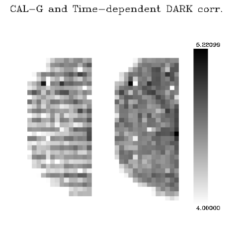
Figure 18.  : The calibration observation of the star HIC85317 done in rev.419, at 6.0^′′PFOV, and T_int =2 sec, with the LW6 filter, reduced using an average dark (left), and the model dark described in this paper (right). Only half of the array is shown in both cases (the star itself is not visible, since it is located on the other half of the array). Flat-fielding was not applied, which explains the vignetting effect at the edges.

The precision of our calibration can be evaluated by computing the residuals of the subtraction of our model dark (eq. 5) from individual calibration darks. From all dark-subtracted dark measurements at a given T_int , we compute the per-pixel RMS. The median RMS is typically $\simeq 0.25$ ADU, similar to the one found for the handover darks  without any temperature and tsa -drift correction, but after the long-term trend correction (see § 3). This is not unexpected, since the handover darks are all done at roughly the same tsa , so there is no need for correcting them for the tsa -drift, and the temperature dependence is generally of minor importance as compared to the revolution and tsa drifts.

We can compare this time- and temperature-dependent dark current correction with that obtained by a simple average of several dark-current measurements, i.e. the “calibration dark” that has been the standard correction applied for all ISOCAM data-reduction until recently. Using the traditional average dark current correction would increase the median per-pixel RMS of the residuals to $\simeq 0.5$ ADU, i.e. twice the value we obtained using the model dark.

In practice, using our dark model in the data-reduction of ISOCAM observations, greatly improves the quality of the images as compared to the traditional data-reduction (when a simple average of several dark current observations was used). This is illustrated in the following examples.

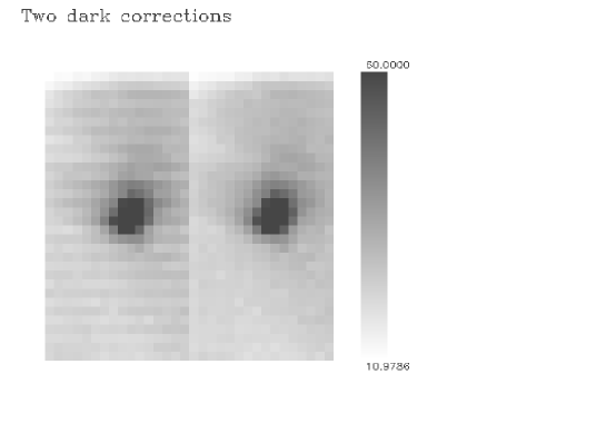
Figure 19.  : The image of a comet, observed in rev.341, with T_int =0.28 sec, with the LW9 filter. The observed data have been reduced using a simple average of many darks (left), and using the model dark described in this paper (right). Only the central half of the array is shown in both cases. The images are shown before flat-fielding.

Figure 20.  : The flux along a single column of the comet image shown in Fig. 19. Upper panel: after subtraction of an average calibration dark. Lower panel: after subtraction of the model dark described in this paper.

In Fig. 18 we provide an example of a specific calibration observation of a star, at T_int =2 sec. The data-reduction was done first by using an average dark correction, and then using our model dark correction. The odd/even line pattern is only evident in the image reduced with the average dark, indicating a poor dark correction.

Another example is given in Fig. 19, where we show the image of a comet observed at T_int =0.28 sec. Again, the odd/even line pattern is evident when we apply the average dark subtraction but not anymore when our dark model is used. To have a quantitative feeling of the accuracy of the dark correction, we plot in Fig. 20 the fluxes measured along the pixels of a single column of the ISOCAM detector, so to emphasize the line pattern. The residual is $\sim 2$ ADU/s (i.e. 0.6 ADU, since T_int =0.28 sec) when the average dark subtraction is applied, while it is less than 1 ADU/s ($\sim 0.2$ ADU) when the dark model subtraction is applied, consistently with the estimates given above.

As a final example, we show in Fig. 21 and Fig. 22 two images of a galaxy at 100 Mpc distance, observed witt a pixel-field-of-view of 1.5^′′  in the LW2 filter, at T_int =2 sec. As before, the two images have been obtained using two kind of dark corrections in the data-reduction: an average of several calibration darks  in Fig. 21 and our dark model in Fig. 22. The dark current subtraction is not perfect even when using our dark model, but it is anyway much better than the one obtained with a simple average dark.

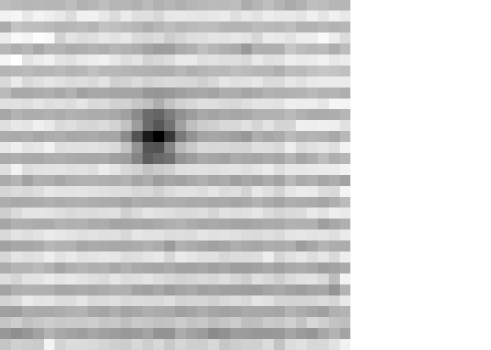
Figure 21.  : The final reduced image of a 100 Mpc distant lenticular galaxy, observed in rev.617, in the LW2 filter, with 1.5^′′  pixel-field-of-view, at T_int =2 sec. The dark used in the data-reduction is an average of several calibration darks.

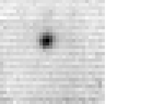
Figure 22.  : The final reduced image of the same observation of Fig. 21, with the dark model used in the data-reduction, instead of an average calibration dark.

7 Conclusions

We have shown that there are several effects that contribute to modify the dark current of the ISOCAM/LW detector during the ISO mission. In particular, we have identified:

• a long-term drift, i.e. a linear decrease of the dark current from a revolution to another, with a typical time-scale of days; this drift is different for different pixels and different T_int ’s;

• a short-term drift, i.e. a modification of the dark current within a single revolution, from the beginning of the revolution to the end; this drift is in general non-linear, and is different for different pixels and different T_int ’s;

• a correlation of the dark current with the temperature of the ISOCAM focal-plane; to the current level of understanding, this correlation is unique, the same for all pixels, and indipendent of the T_int .

We can summarize as follows the impact of each of these effects on the dark-current:

• long-term trend: the drift is $\sim-2$ ADU from the beginning to the end of the ISO mission;

• short-term trend: the drift within each revolution is $\sim\pm 0.5$ ADU from the activation to the de-activation of the ISOCAM instrument;

• temperature-dependence: $\sim\pm 0.25$ ADU over the full range of temperature variation (few hundreths of a kelvin).

Correcting for all these effects is clearly important. We have modelled them using polynomial fittings of the available dark current data, taken under many different conditions (during the handover, during prime-mode calibration revolutions, and with ISOCAM operating in parallel-mode). The result is a dark-model, dependent on three variables, the number of the revolution, the time of observation within that revolution (counted since the instrument activation), and the temperature of the ISOCAM detector. The dependence is different for different pixels, and slightly different for different T_int ’s. Note that the temperature-dependence, at variance with the revolution and tsa dependences, is assumed to be the same for all T_int ’s and all pixels, although we are aware that future (more detailed) analyses may lead us to drop this assumption.

Once corrections are applied, the median LW dark current residual amounts to $\simeq 0.25$ ADU, which is even better than the pre-launch estimate of 0.3 ADU (see, e.g., Biviano 1998).

The success and simplicity of this modelisation of the ISOCAM/LW dark-current behaviour has prompted its implementation in the CIA package for the ISOCAM data-reduction (version 3.0; Delaney 1998) and in the Off-Line Processing of the ISOCAM data (version 6.0; see, e.g., Siebenmorgen et al. 1998). As we have shown in § 6 this represents a significant improvement in the data-reduction of ISOCAM data, as compared to the traditional approach which used a simple average of many calibration darks, as the reference calibration dark.

8 References

References

- [] Biviano A. 1998, “The ISOCAM Calibration Error Budget Report”, available at http://www.iso.vilspa.esa.es/users/expl_lib/CAM_top.html
- [] Delaney M. ed. 1998, “ISOCAM Interactive Analysis User’s Manual”, Version 3.0, available at http://www.iso.vilspa.esa.es/users/expl_lib/CAM_top.html
-
[]
Gallais P., Boulade O. 1998, “Report on the Trend Analysis of the CAM
Daily Calibrations Measurements”, available at
http://www.iso.vilspa.esa.es/users/expl_lib/CAM_list.html - [] Ott S. et al. 1996, “Design and Implementation of CIA, the ISOCAM Interactive Analysis System”, ASP Conference Series, Vol. 125, available at http://www.iso.vilspa.esa.es/users/expl_lib/CAM_top.html
- [] Siebenmorgen R., Starck Jean-Luc, Sauvage M., Cesarsky D., Blommaert J., Ott S. 1998, “ISOCAM Data Users Manual”, Version 4.0, available at http://www.iso.vilspa.esa.es/users/expl_lib/CAM_top.html
- [] The ISOCAM Team 1995, “Observer’s Manual for ISOCAM”, available at http://www.iso.vilspa.esa.es/users/expl_lib/CAM_top.html