Topological Defects and CMB anisotropies : Are the predictions reliable ?

Abstract

We consider a network of topological defects which can partly decay into neutrinos, photons, baryons, or Cold Dark Matter. We find that the degree-scale amplitude of the cosmic microwave background (CMB) anisotropies as well as the shape of the matter power spectrum can be considerably modified when such a decay is taken into account. We conclude that present predictions concerning structure formation by defects might be unreliable.

I Introduction

Two challenging paradigms to explain structure formation in the Universe are currently developped, namely cosmological inflation [1] and topological defects [2]. On the one hand, inflation is a simple theory, based on the linear evolution of acausal and coherent initial perturbations produced during an accelerated phase of expansion of the early Universe. Several public codes are available, notably CMBFAST [3], to compute the CMB anisotropies of a given model in few minutes, and these predictions are robust. On the other hand, topological defects, which are supposed to have formed after a cosmological phase transition in the early Universe, are much more difficult to handle, because of the highly non-linear structure of their dynamics. After some pioneering work by Bennett, Bouchet, Stebbins [4], Shellard, Allen [5], Perivolaropoulos [6], Caldwell et al. [7], the first detailed predictions of some defect models have been published only recently. In particular, Turok, then Pen, Seljak and Turok [8] have considered global defects, as well as Durrer and collaborators [9] who studied more carefully the large $N$ limit. Following Vincent, Hindmarsh and Sakellariadou [10], Battye, Albrecht and Robinson [11], have studied a network of line-like segments with given correlation length and velocity distribution, as well as Pogosian and Vachaspati [12] who also considered the wiggly structure of the strings. Allen, Shellard and collaborators [13], and Contaldi, Hindmarsh and Magueijo [14] have considered local cosmic strings.

Several ground experiments (Saskatoon, Python V, TOCO, see [15]; see also [16] for an up-to-date compilation of the current results) have by now probed the degree-scale anisotropy of the microwave sky. They seem to indicate the presence of a high peak in the spectrum. Now, in contradiction with these observations, topological defect models do not produce generically much more power on the degree scale than on the largest scales observed by the COBE satellite [17]. The reason is that, although the defects evolve according to causal processes, thus producing power on small angular scales on the last scattering surface, one must also take into account their gravitational interaction with the photons after last scattering. This so-called Integrated Sachs-Wolfe effect (see e.g. [18]), known to be negligible in most inflationary scenarios, greatly increases in the case of defects the power on large angular scales, thus contradicting the present observations (see however [12], where the wiggly structure of strings is properly taken into account, yielding more power on the degree scale). Moreover, in most defect theories, the situation is also worsened by the fact that scalar, vector and tensor modes all contribute significantly to the overall CMB anisotropies, whereas only the scalar contribution is expected to produce more power on small angular scales than on larger ones.

It must however be stressed that, in all the numerical defect models already mentionned, an important physical effect, to wit their decay into gravitational radiation and/or elementary particles, has been considered in most cases in a phenomenological way only (but see however [19]). Turok et al. and Durrer et al. have imposed and checked that their global defect stress-energy tensor is conserved. In cosmic string numerical simulations one has to deal with the problem of loop production and evolution, which has been treated in various ways. Turok et al. have introduced an extra radiation fluid into which their cosmic string loops are supposed to decay, Battye et al. have introduced an extra fluid with given constraints on its stress-energy tensor, and Magueijo et al., whose stress-energy tensor is not conserved due to the fact that the smallest loops are extracted out of the simulation, “dump” the string energy losses into either extra-fluids with no anisotropic stress and various equations of state, or in one or the other of the existing background fluids, that is the baryons, photons, neutrinos or CDM. Finally, Shellard et al. treat the loops as relativistic point masses, and Pogosian et al. treat them as small segments.

The aim of this paper is first to show that the microphysics of defects imposes that energy be released in the cosmic fluids and that the predictions concerning the CMB anisotropies change drastically when even a small fraction of the network energy is released directly in the form of photons or baryons, and, to a lesser extent, neutrinos. As for the matter power spectrum, we will see that it is greatly affected if the network energy is released into photons, neutrinos, or baryons.

Such a lack of generic predictive power for seeds-based models has already been pointed out in another context by Durrer and Sakellariadou [20], who have used various ansa̋tze for the stress-energy tensor components of scaling coherent seeds and have found a wide variety of results for the positions and heights of the induced CMB anisotropies Doppler peaks. One could argue that these results were obtained by using very ad-hoc hypothesis for the seeds correlators, but at least three other works have reached similar conclusions by using more realistic models. Perivolaropoulos [6] has pointed out that a correct modelling of the gravitational interaction between cosmic strings wiggles and electrons could induce more small scale anisotropies than previously expected, and this analysis was confirmed by the more precise numerical works of Pogosian and Vachaspati [12]. Finally, the inclusion of decay products in the specific model of Contaldi et al. [14] proved to have an important effect on the CMB anisotropies spectrum. Interestingly enough, these two models which add some small-scale physics give a better agreement with observations than those which do not include any small-scale physics. We show here that such effects are not restricted to any specific model but hold for a very large class of defects and decay processes.

We shall first discuss the microphysics behind such effects, then show how one can generically take them into account, and finally present some results.

II The decay products of realistic string models

Topological defects fall in various classes [2].

Uncharged Goto-Nambu strings form loops which are usually supposed to decay dominantly into gravitational radiation [21, 22], thus guaranteeing the scaling behaviour of the network (that is the fact that the ratio of the energy density contained in the network with the total energy density is constant in time). This extra gravitational radiation added to the background is observationally constrained by e.g. the millisecond pulsar timing measurements [23].

Uncharged global strings, when seen from a distance, appear very much like local ones, but with an energy per unit length renormalized to include long-range interaction effects [24]. The overall global string network is therefore expected to behave much like a Goto-Nambu network, except for the small loops [25]. The main difference between a local and a global string loop is that while the former is supposed to radiate mostly in gravitational waves, the latter looses energy mainly through massless Goldstone boson radiation, a process known to be far more efficient [25]. This new extra component added to the background is only constrained by nucleosynthesis [26].

The last potentially interesting class of strings in the context considered here is that of Grand-Unified (GUT) superconducting cosmic strings [27] (only GUT strings can be relevant in large scale structure formation and CMB fluctuations). Again, their network evolution is almost the same as that of Goto-Nambu strings because most of the evolution takes place when the currents flowing along the strings are negligible [28]. This is however true only for infinite strings or for those having very large radius of curvature.

When a superconducting loop decays, its energy can be very efficiently released in the background directly in the form of electromagnetic radiation [29]. The electromagnetic radiation cannot propagate because of the surrounding plasma, the influence of which cannot be neglected. The waves form shells where energy is concentrated. These shells are the basis for the explosive Ostriker, Thompson and Witten large scale structure formation model [30] and yield a distorsion in the microwave background by modifying its spectrum, implying non zero values for the parameters $\mu$ (chemical potential distortion, see e.g. [31]) and $y$ (characterizing the Sunyaev-Zel’dovitch effect, see e.g. [32]). This very stringent constraint, together with e.g. nucleosynthesis constraints [33] almost rules the scenario out, leaving as the only possibility that the radiation can only be emitted at much higher frequencies (to allow propagation in the plasma). This requires that the strings can be considered current-free until they have shrunk to a sufficiently small size, the wavelength of the radiation being proportional to the emitting loop radius. As a result, one can consider the network evolution as, again, that of a Goto-Nambu network with the difference that part of the energy contained in the loops can now be transferred directly into the photon fluid.

When such a loop shrinks however, the integrated current being conserved, the energy it contains per unit length increases and its effects become more and more important on the string dynamics. The resulting loop distribution can accumulate to stationary states known as vortons [34]. This overproduction of vortons breaks the scaling behaviour of the network, thus leading to such a cosmological catastrophe that one must assume that the vortons are sufficiently unstable to decay in less than one Hubble time.

The new phenomenon one therefore needs to consider is the fate of the small charged loops. As discussed above, they can decay into gravitational radiation, or directly into photons. The third, largely overlooked possibility when it comes to compute CMB anisotropies or matter power spectrum, is that they might decay into their constituents [35], namely massive Higgs and gauge bosons and the particles they couple to and that make the current, collectively referred to as “$X$”-particles. As these particles have masses comparable to the grand unification scale, their decay products can only be estimated by the relevant QCD extrapolations at high energy [36]. The standard scenario is that the primary $X$-particle will decay into a lepton (usually an electron) and a quark which subsequently initiate a hadronic shower. Once the shower has evolved, one ends up with roughly $3$% nucleons [36], and the rest in $\pi$’s, which, because of their decays or interactions with other background fluids, turn into neutrinos, photons and electrons. These interactions have even been used to try and explain the ultra high energy cosmic ray [37] enigma by means of topological defects [38]. Note that this picture does not take into account the possibility that part of the decay product be a stable particle, i.e. a constituent of the dark matter. The Lightest Super Particle is a possible candidate, for instance if SUSY is demanded, as should be the case for any GUT model.

This analysis of small superconducting loops has led us to conclude that they mostly decay (hence ensuring that their network scales) directly into the constituents of the universe rather than into extra-fluids such as gravitational radiation.

In fact one can also argue that non superconductiong strings, because they intercommute, can also partly decay into photons, baryons, neutrinos or dark matter, and not only into gravitational radiation or Goldstone bosons for the global ones. Even global defects can also decay [2] : when the gradients are strong enough high energy particles and gravitational radiation are produced. One might expect however that the energy losses in the form of background fluids be far more efficient for superconducting, rather than uncharged, defects.

III A two-parameters decay model

When one solves the classical (Goto-Nambu) equations of motion for the string network in a Friedmann-Robertson-Walker (FRW) background, completed by a set of rules which fixes the intercommutation of long strings into loops, in the stiff approximation [39] framework (in which the defect network energy is a first order perturbation to the FRW background), and if no extra physics is added to the problem, the corresponding stress-energy tensor of the strings must be covariantly conserved. If it is not, that only means that the numerical integration is not precise enough. The same holds true for global defects.

Now, as we have seen in §II, extra physics must be added. Indeed intercommutation leads to the formation of more and more small loops per Hubble volume which would prevent scaling to take place and soon dominate the evolution of the universe, were they not eliminated by turning into gravitational radiation and/or various elementary particles. The string stress-energy tensor cannot then be conserved. This is particularly clear in numerical simulations when loops smaller than a given size are phenomenologically extracted by hand from the network (as in e.g. [14]).

In the semi-analytic approach we use here (see below), we model active seeds by a stress-energy tensor $\Theta^{s}_{\mu\nu}$ which, from the start, embodies the scaling properties of the network : first, deep in the radiation-dominated or matter-dominated eras, its equal-time correlators $\left<\Theta^{s}_{\mu\nu}({\mathbf{x}},\eta)\Theta^{s}_{\rho\sigma}({\mathbf{x}^{\prime}},\eta)\right>$ depend on $({\mathbf{x}}-{\mathbf{x}^{\prime}})/\eta$ only, second they vanish at small scales ($\eta$ is conformal time and $x^{i}$ are comoving coordinates). Therefore this effective stress-energy tensor describes in fact, not only the defects themselves but also their decay products, as long as these decay products are themselves “seeds”, that is an active perturbation added to the background fluids. Now among the possible decay products described in §II, only the gravitational and Goldstone radiations enter in that category. Hence, if the defects were scaling only via the production of this “extra” radiation, the effective stress-energy tensor we use, being the sum of the stress-energy tensor of the defects and that of the extra radiation they produce, would be conserved. In contrast, in numerical simulations where the defect stress-energy tensor is not conserved, such decay products must be treated as an extra fluid with given equation of state.

However, as we have seen, in the case of superconducting strings at least, loops decay mainly through the emission of high energy particles which soon turn into (mostly) neutrinos and photons, which must be added to those already existing in the background. Therefore we shall describe the defects by an effective stress energy-tensor which will not be conserved in order to take into account the decay of the loops into high energy particles, and we shall dump the string energy losses not in an extra component but into the background fluids.

In the semi-analytic approach initiated by Durrer and collaborators [9], the defect network and the extra “seeds” they decay into are modelled by a stress-energy tensor $\Theta_{\mu\nu}^{s}$ which acts as a source for the linearized Einstein equations and induces inhomogeneities in the cosmic fluids. The ten components of this stress-energy tensor are then drastically constrained by a number of physical requirements [40, 41, 42], which take into account that the seeds :

1. are statistically homogeneous and isotropic,

2. are created at a phase transition in an up to then perfectly homogeneous and isotropic universe (hence obeys specific causality [40] and matching [41] conditions),

3. evolve deep in the radiation era and deep in the matter era in a way which is statistically independent of time (scaling requirement [42]).

One can now suppose that the defect network is made of long strings of comoving curvature radius $R_{L}>1/{\mathcal{H}}$ (${\mathcal{H}}$ is the comoving Hubble parameter), which eventually interconnect so as to form loops. When they become too small these loops decay at a certain rate (depending on the details of the decay processes). The loss of energy of the stress-energy tensor can therefore, in a rough approximation, be modelled as

$$D_{\mu}\Theta_{s}^{\mu\nu} = F^{\nu},$$ (1)

$$\hat{F}^{\nu}=-\dot{\mu}\hat{\Theta}_{s}^{0\nu} \quad\mathrm{with}\quad \dot{\mu}=\Gamma Y(k-k_{c})$$ (2)

where $D_{\mu}$ is a covariant derivative (we assume flat spatial section), a hat denotes a Fourier transform, $Y$ is the Heavyside function, $k\propto 1/R_{L}$ is the comoving wavenumber. $\Gamma$ is a free function which determines the decay rate of the loops into the decay products, and $k_{c}$ is the scale above which the loops begin to decay. This $\hat{F}^{\nu}$ is then injected into the other fluid perturbation equations with branching ratios $x_{f}$, so as to ensure that the total stress-energy tensor is conserved (see appendix A for the actual equations we solve). The branching ratios $x_{f}$ are in principle calculable when the decay microphysics is explicited.

IV Results

A CMB anisotropies

We have computed numerically the CMB anisotropies and the matter power spectrum such decaying seeds produce. We first summarize our findings before going into discussing them. Dumping energy into CDM has negligible effect on the CMB anisotropies spectrum. Dumping energy into neutrinos has a relatively small influence on the spectrum, which is modified by a few tens of percent. This can either increase or decrease the amplitude of the spectrum [we have found that this depends on the parameters of the decay term (2), as well as on the ansa̋tze for the correlators (A6,A7)]. On the contrary, the spectrum is tremendously affected by injecting energy into either photons or baryons, although the effect is much stronger when one injects energy directly into photons, which can boost the degree-scale amplitude of the spectrum by a factor as large as 50. The precise amplitude of the boost depends of course on the underlying defect model, but all those we have checked present the same qualitative features.

A simple interpretation of these results is that energy, when injected into either neutrinos or CDM, influences the photons perturbations only through gravity, so that the influence of this energy injection on the CMB anisotropies is small. On the opposite, by dumping energy into baryons or photons, one directly affects the evolution of the perturbed photons density and/or velocity since photons and baryons are strongly coupled through Thomson diffusion before recombination. The angular scale at which this effect is strongest is given by the angular size of the “decay scale” (i.e. the Hubble radius when $k_{c}={\mathcal{H}}$) at the last scattering surface, that is $\theta\simeq 1\deg$.

For example in Fig. 1, we consider the scalar contribution to the CMB anisotropies of a specific coherent model where we have chosen the equal time correlators for the pressure and the anisotropic stress [see eqns. (A6,A7)] in such a way that they respect the standard causality and scaling requirements (see appendix for more details). We have also chosen the relative amplitudes of the correlators so that, when the stress-energy tensor is conserved, we “mimic” the situation of more realistic incoherent numerical defect models (i.e. the CMB anisotropies spectrum lacks power on the degree-scale with respect to observations; the coherent model presented here exhibits acoustic oscillations which are expected to be smoothed out by decoherence, see [8]). The two parameters of the decay model, $k_{c}$ and $\Gamma$ [see eq. (2)] have both been chosen equal to ${\mathcal{H}}$. We have also studied many other models such as the “pressure model” [43] [where ones sets the anisotropic stress $\hat{\Pi}^{s}$ to 0, see eqns. (A6,A7)], or the “anisotropic stress model” (where the pressure $\hat{P}^{s}$ is set to 0, see e.g. [44]), which all yield similar qualitative results. In all what follows, the CMB data points are taken from [16] and the matter power spectrum data points are those of the APM catalog [45] and of Dekel et al. [46].

In Figs. 2 and 3 we study the influence of the parameters $k_{c}$ and $\Gamma$ for the model of Fig. 1 where energy is equally released into photons or neutrinos. By increasing $k_{c}$ (Fig. 2), which gives essentially the wavenumber scale at which energy is injected, we get that, as expected, the spectrum is enhanced on smaller angular scales, i.e. the bump is shifted to the right. On the contrary, by increasing $\Gamma$ (Fig. 3), namely the defects decay rate, energy is transferred more rapidly into the background fluids, and therefore at larger wavelengths. The spectrum is thus enhanced on larger angular scales, so that the bump is shifted to the left.

B Matter power spectrum

Dumping energy into CDM has also negligible effect on the (baryonic) matter power spectrum. On the contrary, the spectrum is strongly affected by injecting energy into either photons or neutrinos. It has the consequence of reducing the excess of energy on small scales, because of the free streaming of these relativistic particles (see e.g.[47]). Finally, injecting energy into baryons gives an intermediate result. Fig. 4 summarizes these results by showing the matter power spectrum corresponding to the model of Fig. 1.

C Observational constraints

In all these numerical analysis, we have assumed that the radiation emitted by the high energy decay product is immediately thermalized as soon as it is produced. However this is only an approximation. Three unwanted effects can be caused by this radiation. First, the radiation emitted before the last scattering surface may not have had the time to thermalize, thus leading to a distortion of the CMB black-body spectrum; this would be the case if too much energy is injected between $z\simeq 10^{6}$ and $z\simeq 10^{3}$. However we inject a small amount of energy compared to that already contained in the CMB (roughly $10^{-6}$ per Hubble time since one is in the radiation-dominated era), so that (considering the current observational bounds on the $\mu$ and $y$ parameters) one can assume it had time to thermalize, see [31]. Second, the radiation emitted after the last scattering surface will not be thermalized, and therefore could produce an important $\gamma$-ray background [33]. Third, the high-energy particles could photo-dissociate the ⁴He nuclei, thus producing lighter nuclei such as ³He and D, which in turn can produce too much ⁶Li [48].

These three effects are already constrained by the observations of the CMB spectrum, the diffuse $\gamma$-ray background and the light elements abundances, but our scenario still happens to be tenable, as shown on Fig. 5 (taken from [33]). In the opposite case, this would disproof most scenario of structure formation seeded by topological defects which dominantly decay into photons.

V Conclusion

We have included some microphysics, up-to-now largely overlooked, in the description of topological defects. This microphysics deals with the decay of defects, and notably superconducting cosmic strings, into background fluids, rather than gravitational radiation as usually assumed. This decay has important observational consequences, which may (depending, of course, on the exact interaction one considers) put the defect models in a better position when confronted to the current observational data.

One could of course argue that the simple model we have considered here (coherent seeds, crude interaction term) is too naive, however our purpose was mainly to illustrate the consequences of this idea rather than to study a more specific realistic model, which we keep for later work. Since the main consequences of dumping energy into the background fluids do not seem to depend too much on the details of the equal time correlators we have considered, but rather on the details of the interactions, we strongly advocate for a more careful study of the branching ratios.

Let us recall that even in inflationary models the inclusion of microphysics and interaction between fluids is absolutely crucial in order to make accurate predictions. For example, if one neglects these by not solving the exact Boltzmann equation for the photons and/or the neutrinos, or by not solving the accurate kinetic recombination equations, one finds an large excess of power at small angular scales (see e.g. Fig. 4 of [18]).

It is therefore clear that predictions of topological defect models concerning structure formation not only require today’s state-of-the-art heavy detailed numerical simulations, but also a rigorous description of their non gravitational interactions before reliable conclusions can be drawn.

Alain.Riazuelo@obspm.fr 
Nathalie.Deruelle@obspm.fr 
Patrick.Peter@obspm.fr

A CMB anisotropies calculations

We assume standard cosmological parameters : flat Universe without cosmological constant, baryon density and Hubble parameter such that $\Omega_{b}=0.05$, $h=0.5$, three massless neutrinos and standard recombination.

The stress-energy tensor of the seeds can be decomposed as a sum of scalar, vector and tensor [49] random fields. The scalar part, the only one we shall consider here, can be written in terms of four random fields $\hat{\rho}^{s}$, $\hat{v}^{s}$, $\hat{P}^{s}$ and $\hat{\pi}^{s}$, as :

$$K\hat{\Theta}_{00}^{s} \equiv \hat{\rho}^{s},$$ (A1)

$$K\hat{\Theta}_{0i}^{s} \equiv -ik_{i}\hat{v}^{s},$$ (A2)

$$K\hat{\Theta}_{ij}^{s} \equiv \hat{P}^{s}\delta_{ij}+\left(\frac{1}{3}k^{2}\delta_{ij}-k_{i}k_{j}\right)\hat{\Pi}^{s}.$$ (A3)

($K$ is Einstein’s constant.) To compute the CMB anisotropies, we need the two-point correlators of the stress-energy tensor. The homogeneity of the distribution imposes :

$$\left<\hat{\Theta}^{s}_{\mu\nu}({\mathbf{k}},\eta)\hat{\Theta}^{s}_{\rho\sigma}({\mathbf{k}^{\prime}},\eta^{\prime})\right>=\delta({\mathbf{k}}-{\mathbf{k}^{\prime}})\hat{C}_{\mu\nu\rho\sigma}({\mathbf{k}},\eta,\eta^{\prime}),$$ (A4)

where the ${\mathbf{k}}$-dependence of $\hat{C}$ is fixed by the requirement that the distribution is isotropic. The correlators can be decomposed as sums of “coherent eigenmodes” [8] :

$$\hat{C}_{\mu\nu\rho\sigma}({\mathbf{k}},\eta,\eta^{\prime})=\sum_{(i)}\lambda^{(i)}\hat{c}_{\mu\nu}^{(i)}({\mathbf{k}},\eta)\hat{c}_{\rho\sigma}^{(i)}({\mathbf{k}},\eta^{\prime}),$$ (A5)

where the $\hat{c}_{\mu\nu}^{(i)}({\mathbf{k}},\eta)$ are the correlators of coherent sources. The four random fields that describe coherent sources are all proportional to the same normalised random variable $e({\mathbf{k}})$ and hence are described by four random fields. Two of these functions are constrained by eqns. (1-2), and the two other must be either imposed by hand or determined using some more detailed modelling. We take simple ansa̋tze for the pressure $\hat{P}^{s}$ and the scalar anisotropic stress $\hat{\Pi}^{s}$, in practice (up to a normalization constant) :

$$\hat{P}^{s} = \eta^{-\frac{1}{2}}\exp(-k^{2}\eta^{2})e({\mathbf{k}}),$$ (A6)

$$\hat{\Pi}^{s} = -4\eta^{-\frac{1}{2}}(k^{2}\eta^{2})\exp(-k^{2}\eta^{2})e({\mathbf{k}}).$$ (A7)

This (rather arbitrary) choice of correlators satisfies the requirements imposed by causality, scaling, etc [42], and is tailored in order to obtain a CMB anisotropies spectrum which lacks power on the degree scale. Of course, the precise shape of these functions can in principle be obtained by numerical simulations, and the CMB anisotropies are known to depend very much on the shape of these free functions [20], but, as already stressed, we have carefully checked that the effect we are interested in does not qualitatively depend on them.

We solve (in the flat-slicing gauge) the well-known (see e.g. [41, 42, 50]) linearised Einstein equations which couple the seeds network to the cosmic fluid inhomogeneities, corrected by the decay term (1-2). They read :

$$\hat{\dot{\rho}}^{s}=-{\mathcal{H}}\hat{\rho}^{s}-3{\mathcal{H}}\hat{P}^{s}+k^{2}\hat{v}^{s}-\dot{\mu}\hat{\rho}^{s} \quad,\quad \hat{\dot{v}}^{s}=-2{\mathcal{H}}\hat{v}^{s}-\hat{P}^{s}+\frac{2}{3}\hat{\Pi}^{s}-\dot{\mu}\hat{v}^{s},$$ (A8)

$$\hat{\dot{\delta}}_{\gamma}=\frac{4}{3}k^{2}\hat{v}_{\gamma}+x_{\gamma}\dot{\mu}\frac{\hat{\rho}^{s}}{3{\mathcal{H}}^{2}\Omega_{\gamma}} \quad,\quad \hat{\dot{v}}_{\gamma}=-\frac{1}{4}\hat{\delta}_{\gamma}+\frac{1}{6}k^{2}\hat{\Pi}_{\gamma}-\hat{\Psi}-\hat{\Phi}-\dot{\kappa}\left(\hat{v}_{\gamma}-\hat{v}_{b}\right)+x_{\gamma}\dot{\mu}\frac{\hat{v}^{s}}{4{\mathcal{H}}^{2}\Omega_{\gamma}},$$ (A9)

$$\hat{\dot{\delta}}_{\nu}=\frac{4}{3}k^{2}\hat{v}_{\nu}+x_{\nu}\dot{\mu}\frac{\hat{\rho}^{s}}{3{\mathcal{H}}^{2}\Omega_{\nu}} \quad,\quad \hat{\dot{v}}_{\nu}=-\frac{1}{4}\hat{\delta}_{\nu}+\frac{1}{6}k^{2}\hat{\Pi}_{\nu}-\hat{\Psi}-\hat{\Phi}+x_{\nu}\dot{\mu}\frac{\hat{v}^{s}}{4{\mathcal{H}}^{2}\Omega_{\nu}},$$ (A10)

$$\hat{\dot{\delta}}_{c}=k^{2}\hat{v}_{c}+x_{c}\dot{\mu}\frac{\hat{\rho}^{s}}{3{\mathcal{H}}^{2}\Omega_{c}} \quad,\quad \hat{\dot{v}}_{c}=-{\mathcal{H}}\hat{v}_{c}-\hat{\Phi}+x_{c}\dot{\mu}\frac{\hat{v}^{s}}{3{\mathcal{H}}^{2}\Omega_{c}},$$ (A11)

$$\hat{\dot{\delta}}_{b}=k^{2}\hat{v}_{b}+x_{b}\dot{\mu}\frac{\hat{\rho}^{s}}{3{\mathcal{H}}^{2}\Omega_{b}} \quad,\quad \hat{\dot{v}}_{b}=-{\mathcal{H}}\hat{v}_{b}-\hat{\Phi}-\frac{4}{3}\frac{\rho_{\gamma}}{\rho_{b}}\dot{\kappa}\left(\hat{v}_{b}-\hat{v}_{\gamma}\right)+x_{b}\dot{\mu}\frac{\hat{v}^{s}}{3{\mathcal{H}}^{2}\Omega_{b}},$$ (A12)

where $\Omega_{f}$, $\delta_{f}$, $v_{f}$, $\Pi_{f}$ are respectively the density parameter, the density contrast, the velocity and the anisotropic stress pertubations for the fluid $f$, the subscripts $b$, $c$, $\nu$, $\gamma$ mean respectively the baryonic, Cold Dark Matter, neutrino and photon fluid, $\Psi$ and $\Phi$ are the two Bardeen gravitational potentials, $\dot{\kappa}$ is the photons differential opacity [51], and a dot denotes a derivation with respect to the conformal time. The terms in $\dot{\mu}$ account for the seeds decay, and the branching ratios $x_{f}$ are constants such that :

$$\sum_{f}x_{f}=1.$$ (A13)

In addition, the two equations for the Bardeen potentials are :

$$2\left[-k^{2}+3(\dot{\mathcal{H}}-{\mathcal{H}}^{2})\right]\hat{\Psi} = 3{\mathcal{H}}^{2}\sum_{f}{\Omega_{f}\left[\hat{\delta}_{f}-3(1+\omega_{f})\hat{v}_{f}\right]}+\hat{\rho}^{s}-3{\mathcal{H}}\hat{v}^{s},$$ (A14)

$$\hat{\Phi} = \hat{\Psi}-3{\mathcal{H}}^{2}\sum_{f}{\Omega_{f}\omega_{f}\hat{\Pi}_{f}}-\hat{\Pi}^{s}.$$ (A15)

Finally, the photons and neutrinos fluids obey a Boltzmann equation which reads (for $\ell\geq 2$, see e.g. [52] or [44] for more details) :

$$\dot{\hat{\Delta}_{\gamma}^{\ell}} = \frac{k}{2\ell+1}\left(\ell\hat{\Delta}_{\gamma}^{\ell-1}-(\ell+1)\hat{\Delta}_{\gamma}^{\ell+1}\right)-\dot{\kappa}\left(\hat{\Delta}_{\gamma}^{\ell}-\delta_{\ell,2}\hat{P}_{\gamma}\right),$$ (A16)

$$\dot{\hat{E}_{\gamma}^{\ell}} = \frac{k}{2\ell+1}\left(\ell\sqrt{1-4/\ell^{2}}\hat{E}_{\gamma}^{\ell-1}-(\ell+1)\sqrt{1-4/(\ell+1)^{2}}\hat{E}_{\gamma}^{\ell+1}\right)-\dot{\kappa}\left(\hat{E}_{\gamma}^{\ell}+\sqrt{6}\hat{P}_{\gamma}\delta_{\ell,2}\right),$$ (A17)

$$\hat{P}_{\gamma} = \frac{1}{10}\left(\hat{\Delta}_{\gamma}^{2}-\sqrt{6}\hat{E}_{\gamma}^{2}\right),$$ (A18)

$$\dot{\hat{\Delta}_{\nu}^{\ell}} = \frac{k}{2\ell+1}\left(\ell\hat{\Delta}_{\nu}^{\ell-1}-(\ell+1)\hat{\Delta}_{\nu}^{\ell+1}\right),$$ (A19)

with $\Delta_{f}^{\ell}$ and $E_{f}^{\ell}$ being respectively the $\ell$-th moment of the temperature and electric-type polarisation distribution functions of the species $f$, and where $P_{f}$ is the coupling between temperature and polarization. The lowest multipoles of the distribution function are related to the perturbed stress-energy tensor components by :

$$\hat{\delta}_{f} = 4\hat{\Delta}_{f}^{0},$$ (A20)

$$\hat{v}_{f} = -\frac{3}{k}\hat{\Delta}_{f}^{1},$$ (A21)

$$\hat{\Pi}_{f} = \frac{12}{k^{2}}\hat{\Delta}_{f}^{2}$$ (A22)

Eqns. (A1-A22) are solved numerically using a Boltzmann code developped by one of us (A.R.) using standard initial conditions [41]. The CMB anisotropies at present conformal time $\eta_{0}$ are then calculated by the line-of-sight integration method [3] :

$$\hat{\Delta}^{\ell}_{\gamma}(k,\eta_{0}) = \int_{0}^{\eta_{0}}\dot{\kappa}e^{-\kappa}\left(\frac{1}{4}\hat{\delta}_{\gamma}+\hat{\Psi}+\hat{\Phi}\right)j_{\ell}(k(\eta_{0}-\eta)){\mathrm{d}}\eta$$ (A23)

$$+ \int_{0}^{\eta_{0}}\dot{\kappa}e^{-\kappa}\left(-k\hat{v}_{b}\right)j^{\prime}_{\ell}(k(\eta_{0}-\eta)){\mathrm{d}}\eta$$ (A24)

$$+ \int_{0}^{\eta_{0}}e^{-\kappa}\left(\dot{\hat{\Psi}}+\dot{\hat{\Phi}}\right)j_{\ell}(k(\eta_{0}-\eta)){\mathrm{d}}\eta$$ (A25)

$$+ \int_{0}^{\eta_{0}}\dot{\kappa}e^{-\kappa}\frac{5}{2}\hat{P}_{\gamma}\left(3j^{\prime\prime}_{\ell}(k(\eta_{0}-\eta))+j_{\ell}(k(\eta_{0}-\eta))\right){\mathrm{d}}\eta.$$ (A26)

In the line-of-sight integration formula (A26), we have omitted the terms arising from the energy injection due to the seeds decay into photons. These terms are proportional to $e^{-\kappa}\dot{\mu}$ and therefore are generated between the last scattering surface and today. The photons emitted because of this decay have therefore very high energy and do not have time to thermalize. Hence, they do not participate to the microwave background, but rather to the diffuse $\gamma$-ray background, which might put some interesting constraints on these models as discussed in §IV C.

Finally, the scalar part of the 2-point correlator of the CMB anisotropies is decomposed as :

$$\left<\frac{\delta T}{T}({\mathbf{n}}_{1})\frac{\delta T}{T}({\mathbf{n}}_{2})\right>_{{\mathbf{n}}_{1}.{\mathbf{n}}_{2}=\cos(\theta)}=\frac{1}{4\pi}\sum_{\ell}(2\ell+1)C_{\ell}^{S}P_{\ell}(\cos\theta),$$ (A27)

where $P_{\ell}$ is the Legendre polynomial of order $\ell$, and the coefficients $C_{\ell}^{S}$ are deduced from the photon distribution multipoles by :

$$C_{\ell}^{S}=\frac{2}{\pi}\int|\hat{\Delta}^{\ell}_{\gamma}(k,\eta_{0})|^{2}k^{2}{\mathrm{d}}k.$$ (A28)

FIG. 1.: CMB anisotropies in a model where the defect stress-energy tensor is not conserved, with $k_{c}=\Gamma={\mathcal{H}}$. The solid line represents the case with conserved stress-energy tensor, as well as the case where one dumps energy into CDM, which are almost identical. The short-dashed and long-dashed lines represent the cases where one dumps energy into neutrinos and baryons respectively. The highest (dotted) line represents the case where energy is injected into photons. The dot-dashed line (which fits the data points best) shows that by tuning by hand the branching ratios (here, $x_{\nu}=x_{\gamma}=0.5$ and $x_{c}=x_{b}=0$) it is possible to be in much better agreement with the data points. Note that the precise values of the best-fit branching ratios depend on the model one considers.

FIG. 2.: Influence of the decay scale $k_{c}$ on the CMB anisotropies. We use the “best fit” model of Fig. 1, with 50% of the energy relased into photons and another 50% into neutrinos, and we vary the parameter $k_{c}$ from ${\mathcal{H}}$ to $5{\mathcal{H}}$. The solid line represents as in Fig. 1 the case where the seed stress-energy tensor is conserved, and the case $k_{c}=\Gamma={\mathcal{H}}$ corresponds to the dot-dashed curve, also plotted in Fig. 1.

FIG. 3.: Influence of the decay rate $\Gamma$ on the CMB anisotropies. We use the “best-fit” model of Fig. 1, with 50% of the energy relased into photons and another 50% into neutrinos, and we vary the parameter $\Gamma$ from ${\mathcal{H}}$ to $5{\mathcal{H}}$. The solid line represents as in Fig. 1 the case where the seed stress-energy tensor is conserved, and the case $k_{c}=\Gamma={\mathcal{H}}$ corresponds to the dot-dashed curve, also plotted in Fig. 1.

FIG. 4.: Matter power spectrum in the same model as in Fig. 1, with $k_{c}=\Gamma={\mathcal{H}}$. The solid line represents the case where the seed stress-energy tensor is conserved. Dumping energy into neutrinos (short-dashed line) or photons (dotted line) has almost the same effect, whereas dumping energy into CDM (solid line) has again negligible effect. Dumping energy into baryons (long-dashed line) boosts the spectrum on larger scales, whereas it damps it on smaller scales. Note that the sharp bump around $k=10^{-3}$ $h$Mpc^-1 shows the scale at which one injects energy (here, the Hubble radius since $k_{c}={\mathcal{H}}$).

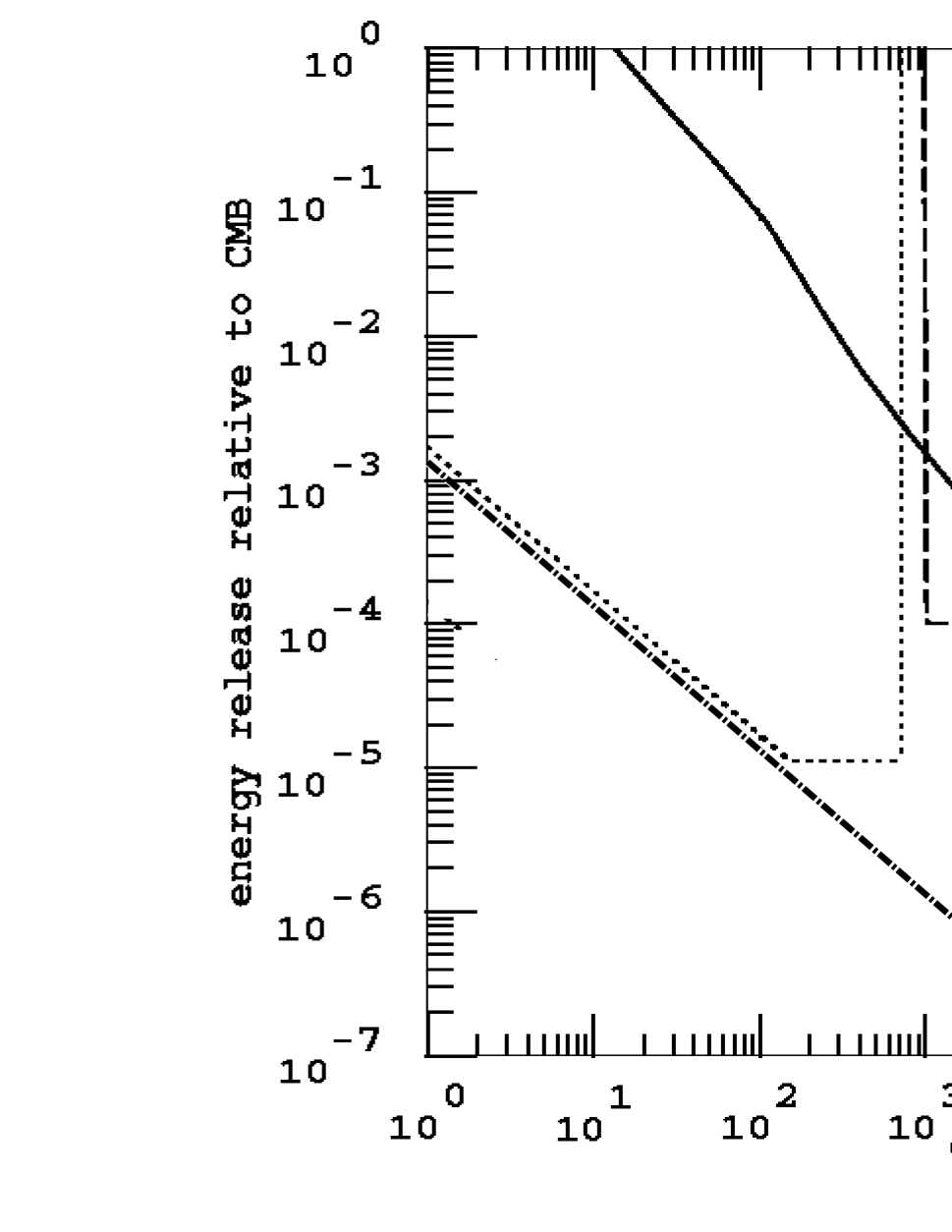
FIG. 5.: Maximal energy release in units of the CMB energy density allowed by the constraints from the observed diffuse $\gamma-$ray background at $5\,$GeV (dotted curve), CMB distortions (dashed curve), and ⁴He photo-disintegration (solid curve) as a function of redshift $z$ (taken from Sigl et al.). These bounds apply for instantaneous energy release at the specified redshift epoch. The lowest (dot-dashed) curve shows the energy release in our model assuming that $\simeq$10% of the energy is released into photons (energy releases into the other fluid do not add to these constraints). Higher energy release into photons might violate the $\gamma$-ray background measurements. Note that the strongest constraint arise today from the diffuse $\gamma$-ray background, but better measurements of the CMB spectrum could give an even stronger constraint.

REFERENCES

- [1] A.H. Guth, Phys. Rev. D23 (1981) 347 ; A.D. Linde, Particle Physics and Inflationary Cosmology, Harwood Academic, New York (1990).
- [2] A. Vilenkin & E.P.S. Shellard, Cosmic strings and other topological defects, Cambridge University Press (1994) and references therein.
- [3] U. Seljak & M. Zaldarriaga, Ap. J. 469 (1996) 437; CMBFAST code is publicly available at URL http://www.sns.ias.edu/~matiasz/CMBFAST/cmbfast.html.
- [4] D.P. Bennett, F.R. Bouchet & A. Stebbins, Nature 335 (1988) 410; D.P. Bennett & F.R. Bouchet, Phys. Rev. D41 (1990) 2408.
- [5] E.P.S. Shellard & B. Allen, “On the evolution of cosmic strings”, in Formation and Evolution of Cosmic Strings, G.W. Gibbons et al. editors, Cambridge University ress (1990).
- [6] L. Perivolaropoulos, Ap. J. 451 (1995) 429-435, astro-ph/9402024.
- [7] B. Allen, R.R. Caldwell, S. Dodelson, L.Knox, E.P.S. Shellard, A. Stebbins, Phys. Rev. Lett. 79 (1997) 2624.
- [8] N. Turok, Phys. Rev. D54 (1996) 3686-3689 astro-ph/9604172; U.-L. Pen, U. Seljak & N. Turok, Phys. Rev. Lett. 79 (1997) 1611-1614, astro-ph/9704165; U.-L. Pen, U. Seljak & N. Turok, Phys. Rev. D58 (1998) 023506, astro-ph/9706250.
- [9] R. Durrer & Z.H. Zhou, Phys. Rev. D53 (1996) 5384; R. Durrer, A. Gangui & M. Sakellariadou, Phys. Rev. Lett. 76 (1996) 579; R. Durrer & M. Kunz, Phys. Rev. D57 (1998) 3199.
- [10] G. Vincent, M. Hindmarsh & M. Sakellariadou, Phys. Rev. D55 (1997) 573.
- [11] A. Albrecht, R.A. Battye & J. Robinson, astro-ph/9707129; A. Albrecht, R.A. Battye & J. Robinson, astro-ph/9711121; R.A. Battye, J. Robinson & A. Albrecht, astro-ph/9711336, and references therein.
- [12] L. Pogosian & T. Vachaspati, Phys. Rev. D60 (1999) 083504, astro-ph/9903361.
- [13] P.P. Avelino, E.P.S. Shellard, J.H.P. Wu & B. Allen, astro-ph/9810439; J.H.P. Wu, P.P. Avelino, E.P.S. Shellard & B. Allen, astro-ph/9812156, and references therein.
- [14] C. Contaldi, M. Hindmarsh & J. Magueijo, astro-ph/9808201; C. Contaldi, M. Hindmarsh & J. Magueijo, astro-ph/9810411, and references therein.
- [15] C.B. Netterfield et al., astro-ph/9601197; K. Coble et al., astro-ph/9902195; E. Torbet et al., Ap. J. 521 (1999) L79-L82, astro-ph/9905100.
- [16] http://www.sns.ias.edu/~max/index.html and references therein.
- [17] G.F. Smoot et al., Ap. J. 396 (1992) L1; C.L. Bennett et al., Ap. J. 464 (1996) L1, astro-ph/9601067.
- [18] W. Hu, in The Universe at high-, Large-scale structure and the Cosmic Microwave Background, E. Martinez-Gonzalez & J.-L. Sanz editors, Springer-Verlag (1996), astro-ph/9511130.
- [19] A. Buonanno & T. Damour, gr-qc/9801105 and references therein.
- [20] R. Durrer & M. Sakellariadou, Phys. Rev. D56 (1997) 4480-4493.
- [21] A. Vilenkin & T. Vachaspati, Phys. Rev. D35 (1987) 1138.
- [22] B. Allen, gr-qc/9604033.
- [23] D.R. Stinebring et al., Phys. Rev. Lett. 65 (1990) 285; V.M. Kaspi et al., ApJ. 428 (1994) 713; S.E. Thorsett & R.J. Dewey, Phys. Rev. D53 (1996) 3468; M.P. Mc Hugh et al., Phys. Rev. D54 (1996) 5993.
- [24] J. Goldstone, Nuovo Cim. 19 (1961) 154.
- [25] F. Lund & T. Regge, Phys. Rev. D14 (1976) 1525; A. Dabholkar & J.M. Quashnock, Nucl. Phys. B 333 (1990) 815; E.J. Copeland, D. Haws & M.B. Hindmarsh, Phys. Rev. D42 (1990) 726.
- [26] R.L. Davis, Phys. Rev. D32 (1985) 3172; Phys. Lett. B 161 (1985) 285.
- [27] E. Witten, Nucl. Phys. B 249 (1985) 557; A.-C. Davis & S.C. Davis, Phys. Rev. D55 (1997) 1879.
- [28] E.J. Copeland, N. Turok & M.B. Hindmarsh, Phys. Rev. Lett. 58 (1987) 1910.
- [29] E.J. Copeland, D. Haws, M.B. Hindmarsh & N. Turok, Nucl. Phys. B 306 (1988) 908.
- [30] J.P. Ostriker, C. Thompson & E. Witten, Phys. Lett. B 180 (1986) 231.
- [31] W. Hu & J. Silk, Phys. Rev. D48 (1993) 485-502.
- [32] Y.B. Zel’dovitch & R.A. Sunyaev, Ap. and Spac. Sci. 4 (1969) 301-316; A. Stebbins, Proceedings of the NATO ASI on the Cosmological Background Radiation, Strasbourg, France, 1996, C.H. Lineweaver et al. editors, Kluwer academic, Dordrecht (1997).
- [33] G. Sigl et al., Phys. Rev. D52 (1995) 6682.
- [34] B. Carter, Ann. N.Y. Acad.Sci., 647 (1991) 758; B. Carter, Proceedings of the XXXth Rencontres de Moriond, Villard-sur-Ollon, Switzerland, 1995, B. Guiderdoni & J. Tran Thanh Vân editors, Frontières, Gif-sur-Yvette (1995); R. Brandenberger, B. Carter, A.-C. Davis & M. Trodden, Phys. Rev. D54 (1996) 6059.
- [35] X. Martin & P. Peter, hep-ph/9808222, to appear in Phys. Rev. D (2000).
- [36] C.T. Hill, Nucl. Phys. B 224 (1983) 469; F.A. Aharonian, P. Bhattacharjee & D.N. Schramm, Phys. Rev. D46 (1992) 4188.
- [37] S. Yoshida et al., Astropart. Phys. 3 (1995) 105; N.N. Efimov et al., ICRR Symposium on Astrophysical Aspects of the Most Energetic Cosmic Rays, M. Nagano & F. Takahara editors, World Scientific (1991); T.A. Egorov, Proceedings of the Tokyo Workshop on Techniques for the Study of Extremely High Energy Cosmic Rays, M. Nagano editor, Institute for Cosmic Rays Research, University of Tokyo (September 1993); J. Linsley, Phys. Rev. Lett. 10 (1963) 146; G. Brooke et al., 19th ICRC (La Jolla) 2 (1985) 150; A.A. Watson, ICRR Symposium on Astrophysical Aspects of the Most Energetic Cosmic Rays, M. Nagano & F. Takahara editors, World Scientific (1991); M.A. Lawrence, R.J.O. Reid & A.A. Watson, J. Phys. G 17 (1991) 733.
- [38] C.T. Hill, D.N. Schramm & T.P. Walker, Phys. Rev. D36 (1987) 1007; P. Bhattacharjee & N.C. Rana, Phys. Lett. B 246 (1990) 365; P. Bhattacharjee, C. T. Hill & D.N. Schramm, Phys. Rev. Lett. 69 (1992) 567; A.J. Gill & T.W.B. Kibble, Phys. Rev. D50 (1994) 3660; P. Bhattacharjee & G. Sigl, Phys. Rev. D51 (1995) 4079; R.J. Protheroe & P.A. Johnson, Astropart. Phys. 4 (1996) 253.
- [39] S. Veeraraghavan & A. Stebbins, Ap. J. 365 (1990) 37.
- [40] N. Turok, Phys. Rev. Lett. 77 (1996) 4138, astro-ph 9607109.
- [41] N. Deruelle, D. Langlois & J.-P. Uzan, Phys. Rev. D56 (1997) 7608.
- [42] J.-P. Uzan, N. Deruelle & A. Riazuelo, astro-ph/9810313.
- [43] C. Cheung & J. Magueijo, astro-ph/9702041.
- [44] W. Hu & M. White, Phys. Rev. D56 (1997) 596-615, astro-ph/9702170.
- [45] C.M. Baugh & G. Efstathiou, Mon. Not. Roy. Astron. Soc. 265 (1993) 145.
- [46] T. Kolatt & A. Dekel, astro-ph/9512132.
- [47] T. Padmanabhan, Structure formation in the Universe, Cambridge University Press (1993).
- [48] K. Jedamzik, astro-ph/9909445.
- [49] J.M. Bardeen, Phys. Rev. D22 (1981) 1882.
- [50] H. Kodama & M. Sasaki, Prog. Theor. Phys. Suppl. 78 (1984) 1; V.F. Mukhanov, F.A. Feldman & R.H. Brandenberger, Phys. Rep. 215 (1992) 203; R. Durrer, Fund. of Cosmic Physics 15 (1994) 209.
- [51] P.J.E. Peebles, Principles of Physical Cosmology, Princeton University Press (1993).
- [52] C.-P. Ma & E. Bertschinger, Ap. J. 455 (1995) 7-25, astro-ph/9506072.