Proto–Galactic Starbursts at High Redshift

Abstract

We have computed the evolving ultraviolet-millimeter spectral energy distribution (SED) produced by proto-galactic starbursts at high redshift, incorporating the chemical evolution of the interstellar medium in a consistent manner. Dust extinction is calculated in a novel way, that is not based on empirical calibrations of extinction curves, but rather on the lifetime of molecular clouds which delays the emergence of each successive generation of stars at ultraviolet wavelengths by typically 15 Myr. The predicted rest-frame far-infrared to millimeter-wave emission includes the calculation of molecular emission-line luminosities (¹²CO and O₂ among other molecules) consistent with the evolving chemical abundances. Here we present details of this new model, along with the results of comparing its predictions with several high-redshift observables, namely: the ultraviolet SEDs of Lyman-limit galaxies, the high-redshift radiogalaxies 4C41.17 and 8C1435, the SCUBA sub-millimeter survey of the Hubble Deep Field (HDF), and the SEDs of intermediate-redshift elliptical galaxies. With our new reddening method, we are able to fit the spectrum of the Lyman–limit galaxy 1512-cB58, and we find an extinction of about 1.9 magnitudes at 1600 Å. This extinction apply to starbursts with spectral slope $\alpha$ in the range $0\lesssim\alpha\lesssim 1.5$. The model also predicts that most Lyman–limit galaxies should have a value of $\alpha$ inside that range, as it is observed. The 850 $\mu$m flux density of a typical Lyman-limit galaxy is expected to be only $\simeq 0.5$ mJy, and therefore the optical counterparts of the most luminous sub-mm sources in the HDF (or any other currently feasible sub-mm survey) are unlikely to be Lyman-break galaxies. The passive evolution of our starburst model is also compared with Keck observations of the reddest known elliptical at $z\sim 1.5$, and with the SED of a typical nearby elliptical galaxy. The SED of the high redshift elliptical is nicely matched by the starburst model with an age of 4 Gyr, and the SED of the nearby elliptical with an age of 13 Gyr.

1 Introduction

Optical surveys of normal and active galaxies have recently begun to provide meaningful constraints on the star formation history of the Universe Madau¡1997¿ ; Dunlop¡1997¿ ; Pettini et al.¡1998¿ ; Steidel et al.¡1998¿ . There is now substantial evidence that the star formation rate grows Madau¡1997¿ ; Pettini et al.¡1998¿ with increasing look-back time out to a redshift of $z\simeq 2$, but calculations of the level of star-formation activity at even higher redshift are still being refined. Initial analyses of the optical image of the HDF indicated a clear decline in star-formation density beyond $z\simeq 1.5$ Madau¡1997¿ , but new sub-mm observations of the HDF with SCUBA Hughes et al.¡1998¿ and new high-redshift Lyman-limit galaxy samples Steidel et al.¡1998¿ , provide little evidence for any clear decline between $z=2$ and $z=4$. Furthermore, it is possible that an important population of high-redshift star-forming galaxies still remains undetected by optical surveys (?), due to being heavily embedded in a significant amount of dust.

The best candidates for high-redshift dust-enshrouded starbursts are objects in which star formation takes place before the gas is able to settle into a disk. It can be argued that these may be the progenitors of present-day elliptical galaxies and bulges, because the stellar populations of elliptical galaxies have properties suggestive of a short (about 1 Gyr or less) formation time-scale, involving a rapid build-up of metals and perhaps dust. Even in the hierarchical galaxy-formation scenario, sub-galactic size clumps are expected to form stars well before these sub-units merge into larger galaxy-size objects (e.g. ?), and the star-formation in these sub-units may be extremely vigorous. In a CDM cosmology small halos will collapse at high redshift ($z>3$) and will have a high initial surface density (e.g. ?). If the star-formation rate is well described at these high redshifts by the Schmidt law Kennicutt¡1998¿ , a straightforward computation shows that they will exhaust their gas in less than 1 Gyr Heavens & Jimenez¡1999¿ , thus one expects these systems to behave like “mini-starbursts” that will quickly form stars. These sub-units will subsequently merge to form the bulges of disks or indeed elliptical galaxies.

In this work we do not therefore refer to a specific model for galaxy morphological evolution, but rather study the properties of generic star-formation bursts that occur at high redshift ($z>3$), and last less than 1 Gyr. Such bursts enrich the interstellar gas to solar metallicity in only 0.2 Gyr, and they might set up strong winds, able to expel most of the gas, in about 0.3–0.8 Gyr.

The purpose of this paper is to present a new self–consistent model for the ultraviolet–to–millimeter spectral energy distribution (SED) of proto-galactic starbursts in which the far–infrared (FIR) dust emission beyond 100 $\mu$m and molecular emission line luminosities are calculated consistently with the radiation field and chemically evolving ISM produced by the rapidly evolving stellar population. These models build on new advances in constructing synthetic stellar populations Jimenez et al.¡1998¿ ; Jimenez et al.¡1999¿ and new three-dimensional simulations of molecular-cloud turbulence, that realistically reproduce the properties of Galactic giant molecular clouds (GMC) Padoan et al.¡1998¿ and allow an accurate modeling of the molecular lines, using a non-LTE radiative transfer code. The model is described in §2 to §5, and some general results are presented in §6. The results of the model are compared with data from galaxies at high redshift in §7, and conclusions are drawn in §8.

2 Synthetic Stellar Population Models

In order to compute the spectro-photometric evolution of starbursts we have used the set of synthetic stellar population models developed by us (?). Our models are based on the extensive set of stellar isochrones computed by ? and the set of stellar photospheric models computed by ? and ?. The interior models were computed using JMSTAR15 (?) which uses the latest OPAL95 radiative opacities for temperatures larger than 8000 K, and Alexander’s opacities (private communication) for those below 8000 K. For the stellar photospheres with temperatures below $8000$ K we have used a set of models computed with an updated version of the MARCS code (U. Jørgensen, private communication), where we have included all the relevant molecules that contribute to the opacity in the photosphere. For temperatures larger than $8000$ K we have used the set of photospheric models by ?. Stellar tracks were computed self-consistently, i.e. the corresponding photospheric models were used as boundary conditions for the interior models. This procedure has the advantage that, since the stellar spectrum is known at any point on the isochrone, the interior of the star is computed more accurately than if a grey photosphere were used, and therefore we overcome the problem of using first a set of interior models computed with boundary conditions defined by a grey atmosphere and then a separate set of stellar atmospheres, either observed or theoretical, that is assigned to the interior isochrone a posteriori. The problem is most severe if observed spectra are used, because metallicity, effective temperature and gravity are not accurately known and therefore their position in the interior isochrone may be completely wrong (in some cases the error is larger than 1000 K). A more comprehensive discussion and a detailed description of the code can be found in ?.

An important ingredient in our synthetic stellar population models is the novel treatment of all post-main evolutionary stages that incorporates a realistic distribution of mass loss. As a result, the horizontal branch is an extended branch and not a red clump like in most stellar population models. Also the evolution along the asymptotic giant branch is done in a way such that the formation of carbon stars is properly predicted, together with the termination of the asymptotic giant branch. In most synthetic stellar population models a constant mass loss law is applied resulting in horizontal branches that are simply red clumps. This leads to synthetic populations that are too red by 0.1 to 0.2 in e.g. $B-R$ (?).

Using the above stellar input we compute synthetic stellar population models that are consistent with their chemical evolution of the interstellar medium. The first step is to build simple stellar populations (SSPs). A SSP is a population of stars formed all at the same time and with homogeneous metallicity. The procedure to build an SSP is the following:

1. A set of stellar tracks of different masses and of the metallicity of the SSP is selected from our library.

2. The luminosity, effective temperature and gravity at the age of the SSP is extracted from each track. Each set of values characterizes a star in the SSP.

3. The corresponding self-consistent photospheric model is assigned to each star.

4. The fluxes of all stars are summed up, with weights proportional to the stellar initial mass function (IMF).

SSPs are the building blocks of any arbitrarily complicated population since the latter can be computed as a sum of SSPs, once the star formation rate is provided. In other words, the luminosity of a stellar population of age $t_{0}$ (since the beginning of star formation) can be written as:

$$L_{\lambda}(t_{0})=\int_{0}^{t_{0}}\int_{Z_{i}}^{Z_{f}}L_{SSP,\lambda}(Z,t_{0}-t)\,dZ\,dt$$ (1)

where the luminosity of the SSP is:

$$L_{SSP,\lambda}(Z,t_{0}-t)=\int_{M_{min}}^{M_{max}}SFR(Z,M,t)\,l_{\lambda}(Z,M,t_{0}-t)\,dM$$ (2)

and $l_{\lambda}(Z,M,t_{0}-t)$ is the luminosity of a star of mass $M$, metallicity $Z$ and age $t_{0}-t$, $Z_{i}$ and $Z_{f}$ are the initial and final metallicities, $M_{min}$ and $M_{max}$ are the smallest and largest stellar mass in the population and $SFR(Z,M,t)$ is the star formation rate at the time $t$ when the SSP is formed.

Our synthetic stellar population models have been extensively used in previous works (e.g. ?; ?; ?; ?), where a detailed comparison with other models in the literature can be found. In this work, we model starbursts assuming that the star formation follows a Schmidt law. In particular, we choose a star-formation law that is proportional to a power of the amount of gas available, $SF(t)=\nu M^{n}$, where we have chosen $n=1.4$ Kennicutt¡1998¿ and $\nu=10$ Gyr^-1, and $M$ is the mass of gas available. Once the star-formation law has been specified, we compute the time evolution of the stellar spectral energy distribution (SED) using the method and the set of SSPs outlined above. In order to compute the chemical evolution of the starburst we have used detailed nucleosynthesis prescriptions and the equations of chemical evolution as described in ?.

3 Dust Emission and Extinction

In the present starburst model the SED is self–consistent from the ultra–violet (UV) to the far–infrared (FIR), because the dust emission is computed on the basis of the UV stellar flux, obtained from the synthetic stellar population calculations. However, the dust extinction of the UV stellar continuum cannot be taken into account in a rigorously self–consistent fashion, and must rely on a specific model, that is not constrained for example by the SED in the FIR region. The ratio of the “observed” FIR and UV luminosities, $L_{FIR}/L_{UV}$, can be $L_{FIR}/L_{UV}\ll 1$, if very little dust is present, or $L_{FIR}/L_{UV}\gg 1$, if a large quantity of dust is present and absorbs a significant fraction of the UV continuum. In the case of local starbursts, ? find that generally $L_{FIR}/L_{UV}>1$, with an average value of about 10, which means that at least 50%, and typically more than 90%, of the UV continuum is absorbed by dust and re-emitted in the FIR. Therefore, if it is assumed that all UV photons are absorbed by dust and re-emitted in the FIR, the FIR luminosity (and SED) can be computed within an uncertainty of less than a factor of two, at least for galaxies that resemble nearby starbursts. On the other hand, such assumption corresponds to $L_{FIR}/L_{UV}=\infty$ ($L_{UV}=0$), and therefore does not allow a realistic computation of $L_{UV}$, or alternatively, a realistic computation of the UV extinction due to dust. In other words, while the FIR SED (or total luminosity) can be computed within an uncertainty of less than a factor of two, by assuming that no UV photons escape out of the starburst, the UV extinction, or the value of $L_{FIR}/L_{UV}$, must be estimated with some more specific model. Depending on the model, the value of the FIR to UV luminosity ratio can be $L_{FIR}/L_{UV}\approx 1$ or $L_{FIR}/L_{UV}\gg 1$. In the sample of local starbursts of ?, more than 1/3 of the galaxies have $10<L_{FIR}/L_{UV}<100$, and, for any given spectral slope, the values of $L_{FIR}/L_{UV}$ span a range of up to two orders of magnitude.

In the following we compute the FIR SED of the dust (§3.1), assuming that all UV photons are absorbed by the dust (for a sufficient total amount of dust), and then develop a novel method to estimate the dust extinction of the UV stellar continuum (§3.2).

3.1 The SED of the “Cold” Dust

Our dust emission model is based on a simplified version of the Draine & Lee dust model Draine & Lee¡1984¿ , and is constructed in a manner similar to that described by ?. Xu & De Zotti use three dust components (cold, warm and hot dust), while we use only one component. The warm and hot dust/molecular components are certainly the most difficult part of the infrared spectrum to model, as they are are dominated by contributions from PAH molecules, optically-thick dust emission from dense gas in clouds, and warm dust emission from HII regions. However, our main interest here is to develop a theoretical tool for the interpretation of future millimeter observations of high-redshift objects, and therefore we avoid the complications of computing the detailed mid-infrared SED and we are concerned only with the spectrum at wavelengths larger than about 100 $\mu$m. In this spectral region the emission is completely dominated by what is commonly referred to as the ‘cold’ dust component.

In our model, as in ?, the same absorption efficiency is used for both graphite and silicate grains. The absorption efficiency for UV photons is taken to be unity, and for optical and far-infrared photons is given by equations (1) and (2) in Xu & De Zotti (1989), which are approximations of Draine & Lee’s results:

$$Q=\frac{X_{\lambda}}{1+X_{\lambda}}$$ (3)

where

$$X_{\lambda}=\frac{2\pi a}{\lambda}$$ (4)

for optical photons;

$$Q_{FIR}=0.065a\lambda^{-1.7}$$ (5)

for FIR photons below 130.9 $\mu$m;

$$Q_{FIR}=0.065a(\lambda/0.013)^{-0.3}\lambda^{-1.7}$$ (6)

for $\lambda>130.9$ $\mu$m. The grain size, $a$, and the wavelength, $\lambda$, are measured in cm. The grain size distribution is a power law,

$$p(a)\propto a^{-3.5}$$ (7)

as in ?, and the number of grains per H–atom is proportional to the metallicity of the gas, $Z$ (unlike in Xu and De Zotti’s model)

$$\frac{n_{gr}}{n_{H}}=3.5\times 10^{-10}(Z/Z_{\odot})({\rm H-atom})^{-1}$$ (8)

where $Z$ is the metallicity of the gas, and the factor $3.5\times 10^{-10}$ is obtained from ?. In our model, the amount of dust is proportional to the metallicity of the gas, and in fact much of the fast initial growth of the far-infrared luminosity of the starburst is due to the build-up of metals. We assume there is no delay between the production of metals and dust, because the dust formation mechanism is not specified in the model. Another major difference between the present model and Xu & De Zotti’s model is that the intensity of the radiation field is not arbitrary, but instead is the result of the computation of the synthetic spectrum of the galaxy.

In order to compute the far-infrared SED of the dust, we calculate the equilibrium temperature, $T_{eq}$, by solving the radiative equilibrium equation for each grain of size $a$:

$$IQ(a)4\pi a^{2}\propto\int{}B_{\lambda}[T_{eq}]Q_{FIR}(a,\lambda)4\pi a^{2}d\lambda$$ (9)

where $B$ is the emissivity of the black body. We then compute the corresponding FIR SED as a superposition of black bodies with the corresponding equilibrium temperatures for each grain.

We do not assume any specific dust or stellar distribution, and therefore we cannot compute the radiation field by calculating the radiation transfer of the UV photons through the dust. We instead assume that both the intrinsic (no dust extinction) stellar radiation field, $I_{0}$, and the actual (extinguished) radiation field to which the grains are exposed, $I$, are uniform:

$$I=gI_{0}=\frac{gL_{gal}}{4\pi R_{gal}^{2}}$$ (10)

where $L_{gal}$ is the galaxy stellar luminosity, from the synthetic stellar population calculations, and $R_{gal}$ is an effective radius, that is of the order of the size of the galaxy, and depends on the stellar distribution. The factor $g$ ($g\leq 1$) is computed by imposing the energy balance between the total UV stellar luminosity and the total FIR dust luminosity. This global energy balance is necessary, because eqn. (9) is the energy balance per grain, and the total FIR dust luminosity is only limited by the total number of grains. We use $g=1$ if the dust luminosity is smaller than the total UV stellar luminosity (the global energy balance is not imposed in this case); we instead impose the global energy balance and determine recursively the equilibrium temperatures and the value of $g<1$, using eqn.s (9) and (10), if the FIR luminosity for $g=1$ would be in excess of the UV luminosity. We do not assume any particular geometrical distribution of the emitting dust, but simply assume that every dust grain experiences the same uniform intensity of the radiation field, $I$, and that the dust emission is optically thin. A better model would require a specific dust distribution, and a radiation field computed as the result of the radiation transfer through that dust distribution. However, the dust distribution is highly uncertain, and therefore we prefer to use simple assumptions, and treat the effective radius, $R_{gal}$, as a parameter of the model. If the FIR dust luminosity is not in excess of the UV luminosity ($g=1$), when $R_{gal}$ is decreased, the intensity of the radiation field and the grain temperature increase. However, $g=1$ only in the very beginning of the star formation process, when the metallicity and the total amount of dust are extremely low. After this transient phase, the radiation field to which the grains are exposed is always extinguished by the dust itself ($g<1$), and practically all UV photons are absorbed by the dust. As a result, the dust temperature is insensitive to $R_{gal}$, because the energy balance yields a value of $g<1$ that keeps the dust temperature constant (in order for the FIR luminosity to not exceed the UV stellar luminosity). Since the parameter $R_{gal}$ has no effect in the model, apart from an extremely short transient phase, we do not discuss it any further. The dust temperature depends only on the total UV luminosity (the star formation history) and on the total number of dust grains. If the stellar luminosity increases, or the total number of grains decreases, the dust temperature increases. Temperature variations occur during the evolution of the starburst (see §6), but they are not very large, because the dust luminosity is proportional to the fourth power of its temperature, according to the Stefan–Boltzmann law.

3.2 Dust Extinction

The interstellar reddening can be computed using reddening laws empirically derived from observational data on nearby starbursts (e.g. ? and references therein). In this work we use an alternative and novel method, that we believe is more appropriate in the interval of wavelengths typically probed by Keck spectra of galaxies at $z\approx 3$, that is between about 1100 and 1700 Å  (cf Lowenthal et al. 1997). We are able to predict the interstellar reddening theoretically, and our main assumption is that star formation at high redshift is a physical process similar to present-day star-formation in our Galaxy, in the sense that most massive stars are formed inside molecular clouds, able to extinguish significantly their far ultra–violet (FUV) flux, until the clouds are eventually dispersed. It might be argued that star formation in protogalactic starbursts must be more efficient than in nearby molecular clouds, where the star formation efficiency is very small. However, even if large molecular clouds only convert 2% of their mass into stars in about $10^{7}$ years, their gas consumption time is $0.5\times 10^{9}$ years, assuming that the gas dispersed after one major star formation episode cools in a time-scale also of the order of $10^{7}$ years. This gas consumption time-scale corresponds to a powerful starburst, if applied to an entire galaxy with a large reservoir of gas. For example, a predominantly gaseous proto-galaxy, with about $5\times 10^{10}$ M_⊙ of gas, and a gas consumption time of $0.5\times 10^{9}$ years, has a star-formation rate of 100 M_⊙/yr.

Infrared surveys in molecular clouds have shown that all massive stars are formed as members of stellar clusters, inside dense molecular cloud cores (e.g. ?; ?). Although isolated star formation does occur in some molecular clouds, such as in the Taurus–Auriga complex, this mode of star formation does not produce massive stars. Massive stars are formed inside dense molecular clouds, and are able to disperse their parent clouds in about $1.5\times 10^{7}$ years, thanks to stellar winds, HII regions and supernova explosions (e.g. ?; ?; ?; ?; ?). Because the life-time of stars of about 15–20 M_⊙ ($Z/Z_{\odot}$=2.5–0.2 respectively) is also about $1.5\times 10^{7}$ years, the FUV radiation from stars bigger than 15–20 M_⊙ is heavily obscured during most of their life-time by their own parent molecular clouds. Examples of young stellar clusters, embedded in molecular gas and dust, are listed in Table 1, together with the fraction of their stars with infrared excess, their estimated age, and their average visual extinction. Stars with infrared excess are believed to still be surrounded by their accretion discs, and so the fraction of infrared excess sources is related to the age of the stellar cluster. Table 1 shows that it is not unreasonable to assume that molecular clouds are the main sources of extinction for the massive stars that they form, for about $1.5\times 10^{7}$ years. There is also observational evidence from external galaxies, that massive stars in starbursts spend a large fraction of their lives buried inside their original molecular clouds Maiz-Apellaniz et al.¡1998¿ .

It is also well known that the distribution of dust in our galaxy is very clumpy, and closely related to the distribution of dense molecular gas (e.g. ?), so it is likely that dust extinction of radiation of massive stars, due to dust distributed outside their parent molecular clouds, is a secondary effect. Note that our assumption is in contradiction with the assumption in ?. There it is assumed that the effect of star formation is to destroy most of the dust in the starburst region, and that the main source of opacity is the dust surrounding the starburst region. According to the assumption of our dust reddening method, stars are being formed inside molecular clouds, that is in dense cold gas that must be associated with dust, and such clumpy dust accounts for most of the dust in the proto-galaxy.

The global UV flux from a galaxy is dominated by the massive stars, especially if the stellar population is young, or in the case of ongoing star formation. Therefore, the global UV flux of a galaxy is strongly extinguished due to the obscuration of massive stars by their parent molecular clouds, while it is affected much less by the possibility that stars smaller than 15–20 M_⊙ are obscured by randomly intervening clouds, after the disruption of their parent cloud. Since the dust distribution is very clumpy, it is to be expected that the dust surface filling fraction of the whole galaxy is significantly less than unity, at significant extinction levels of about $A_{V}\geq 0.5$ mag.

Given the above arguments, we compute the dust extinction in high-redshift proto-galactic starbursts, by allowing all new-born stars to remain dark for $1.5\times 10^{7}$ years. After this period of time the dark cloud is destroyed and stars become visible. The present method ignores the possible effect of dust as a screen acting on all the stellar population, because this is not the dominant effect in our model. The most important property of the present method of computing dust extinction is that it is independent of the total amount of dust in the galaxy. The empirical method proposed by ? is based on the assumption that starbursts have the same stellar populations (age, metallicity, etc.), and that their colors are only due to the amount of dust. A larger amount of dust produces more extinction and redder colors. The same is true for any screen model of dust extinction. In our method, the extinction is computed independently of the amount of dust, and no assumption has to be made about the intrinsic stellar population, so that the properties of the intrinsic stellar population can be constrained by comparing the model with the observations. Results of our reddening method are shown below, where the models are compared with the observed properties of Lyman-break galaxies.

Our way to estimate the extinction is an approximation that is valid mainly in the FUV region of the SED, that is the region probed by Keck spectra of galaxies at high redshift ($z>2.5$). We do not claim that O stars are never observed because totally obscured by their parent molecular clouds. We only note that they are sufficiently extinguished by their parent clouds, so that they are not the main source of FUV photons in a stellar population with a Salpeter IMF. This can be verified empirically in the following way. OB stellar associations are observed in external galaxies (see for example ?) and in the Magellanic Clouds (e.g. ?; ?; ?; ?). The extinction of HII regions, or of their ionizing stars, varies typically in the range $0.2<A_{V}<2.0$ mag. As an example, the extinction of HII regions in the Small Magellanic Cloud (SMC), estimated by ? is in the range $0.28<A_{V}<1.66$ mag, with an average value $<A_{V}>=0.66$ mag. The same authors estimate also the extinction of the ionizing stars, for a sample of HII regions in the SMC that partially overlaps with the previous sample, and obtain values in the range $0.23<A_{V}<0.79$, with an average value $<A_{V}>=0.51$ mag. As a typical extinction we can take for example the global average using both HII regions and their ionizing stars, and we obtain $<A_{V}>=0.65$ mag. In this work we will compare the SED of our model with the SED of Lyman break galaxies (see below), in the FUV region, between 1100 and 1600 Å. Using a standard extinction curve for the SMC (see ? and references therein), $A_{V}=0.65$ mag corresponds to $A_{1300\AA}\approx 2.5$ mag. Therefore, HII regions in the SMC are extinguished by dust so that typically less than 10% of the FUV photons emitted by their ionizing stars can escape. Since about 20% of the total FUV flux of a stellar population with a Salpeter IMF is emitted by stars with mass smaller than 15–20 M_⊙ (and lifetime longer than $1.5\times 10^{7}$ years), stars more massive than 15–20 M_⊙ can contribute only for less than half of the FUV photons that escape dust absorption. This argument assumes that after about $1.5\times 10^{7}$ years most stars will be outside their parent molecular clouds, and not necessarily associated with HII regions, or, in other words, that after $1.5\times 10^{7}$ years $A_{V}\ll 0.65$ mag for the remaining B stars. The extinction measurements towards HII regions in nearby external galaxies confirm therefore the assumption of our extinction method.

4 Molecular Clouds

Molecular lines are computed using models of molecular clouds developed by ?. The molecular emission from the whole galaxy is calculated as the sum of the emission from single model clouds. The relative velocity dispersion of molecular clouds in the gravitational potential of a protogalaxy is likely to be of the order of the galaxy virial velocity, and thus much larger than the internal velocity dispersion of typical molecular clouds. Therefore, it is unlikely that different clouds are seen along the same line of sight with sufficiently similar radial velocities for molecular emission from one cloud to be significantly absorbed by the others. Here we give only a brief description of the calculation of the molecular cloud models, since details can be found elsewhere Juvela¡1997¿ ; Padoan et al.¡1998¿ .

Molecular emission lines are calculated using a non-LTE Monte Carlo radiative transfer code (see below), which solves the radiative transfer problem for any given density distribution, velocity field, radiation field, kinetic temperature distribution, and chemical abundances. The density and velocity fields are calculated by solving the three-dimensional and compressible magneto-hydrodynamic (MHD) equations, in a regime of highly super-sonic isothermal turbulent flows, typical of motions in Galactic molecular clouds Padoan et al.¡1998¿ . The MHD turbulence simulations generate a large density contrast, with the density field spanning 4-5 orders of magnitude. The density field is very intermittent (most mass concentrates in a small fraction of the total volume) and has a filamentary and clumpy morphology (see Fig. 1), reminiscent of real molecular clouds. It has been shown that the density, velocity and magnetic fields generated by these numerical simulations are consistent with several observational constraints Padoan, Nordlund & Jones¡1997¿ ; Padoan et al.¡1998¿ ; Padoan & Nordlund¡1999¿ ; Padoan et al.¡1999¿ , and that super-sonic and super-alfvénic isothermal MHD turbulence is therefore a good model for the dynamics and structure of molecular clouds Padoan & Nordlund¡1999¿ . In this work, a run in a 128³ grid of points is used, with rms Mach number ${\cal M}=15$ and Alfvénic Mach number ${\cal M}_{A}=4$, where ${\cal M}$ is the ratio of the rms flow velocity to the sound velocity, and ${\cal M}_{A}$ is the ratio of the rms flow velocity to the Alfvén velocity. This run is the same as model Ad2 in ?. The isothermal equation of state is used in the MHD equations, and a uniform temperature is also assumed in the radiative transfer calculations, although the Monte Carlo radiative transfer code can deal with any temperature distribution. A range of gas kinetic temperature values between 10 and 60 K has been used, and the cosmic background temperature has been varied between 2.7 and 20 K, according to the assumed redshift for the starburst.

In order to compute the luminosity of molecular lines, the abundance of the molecules must be specified. Molecular chemistry in the context of high-redshift proto-galaxies is discussed by ?, and we refer the reader to that paper for plausible models of the evolution of important molecules, mainly O₂ and CO. The abundance of O₂ is very uncertain, and for simplicity we assume it is proportional to the gas O metallicity, and equal to $1.0\times 10^{-5}$ relative to H₂, at solar metallicity. The CO abundance is approximately equal to the abundance of C if O is more abundant than C, O/C$>$1 (e.g. low metallicity or high star-formation rate), while it is approximately equal to the O abundance if O/C$<$1, since most of the available O is in CO Frayer & Brown¡1997¿ . For the Sun, O/C$\approx 2$, and for the local interstellar medium, O/C=1.2–2.5 Meyer et al.¡1994¿ . Since the chemical evolution is computed self-consistently in our model, C and O abundances are known at any time (see Figure 2), and we can therefore choose to set the CO abundance equal to the C abundance if O/C$>$1, or equal to the O abundance if O/C$<$1 (see ?). As can be seen in Fig. 2, with the star-formation law assumed here it transpires that O/C$>$1 during the whole star-formation episode, and so the CO abundance is simply set equal to the C abundance. Finally, we have assumed that half of the total amount of gas is in molecules, which is reasonable in the light of observational results (e.g. ?). Given these assumptions, the computed luminosity of the ¹²CO lines should be in error by probably a factor of approximately two at most. However, the uncertainty in the luminosity of the O₂ lines is certainly much larger, and there is the possibility that such lines could be 10 times more luminous than the value predicted by the present model.

5 Radiative Transfer Calculations

The non-LTE level populations were solved with a Monte-Carlo method (method B in ?). The radiation field is simulated with a large number of photon packages each representing the distributions of real photons in the different transitions and at different Doppler shifts from the line center. In our method the packages are always started at the edge of the cloud and contain initially only photons from the background radiation field. During the simulation, packages are followed through the cloud along randomly-selected lines and the interactions between photons and gas are calculated. In each cell, the photons that are emitted by the gas are added to the passing package and the number of photons absorbed in the cell is counted. These counters are later used to solve new level populations before the simulation continues with a new set of photon packages. As a photon package exits the cloud the number of photons is recorded. The recorded values represent the luminosity of the cloud in the different transitions integrated over the whole cloud surface.

For the calculations the cubic model cloud was divided into 64³ cells where the density and velocity values were interpolated from the original 128³ data-cube that is the result of the MHD calculations. For each cell the intrinsic non-thermal velocity dispersion was estimated from dispersion of the velocity values in the original data-cube. Together with the thermal line broadening this defines the local absorption and emission profiles for the radiative-transfer calculations. The reduction of the linear resolution by a factor of two (from 128 to 64 grid points) is not expected to affect the results of the radiative-transfer calculations significantly. The density variations are still resolved and most cells remain optically thin. The limited resolution might slightly reduce the emission from transitions between high-energy levels ($J\sim$10) that are populated only in the rarest, densest cells. No such effects are expected for the lower-level transitions which are emitted by much larger regions. This has also been confirmed in previous calculations with similar models.

The model cloud has a linear size of 20 pc and a mean density of 200 cm^-3. The total range of densities extends from just under 1 cm^-3 to 1.25$\times$10⁴cm^-3. The critical density of the CO(1–0) transition, $n_{\rm cr}$=1.8$\times$10³cm^-3, is exceeded in only some 2% of the cloud volume and most of the CO is clearly sub-thermally excited.

The background radiation field consists of CMB at the corresponding redshift (e.g. models discussed below have $T$=15 K corresponding to $z=$4.5) and an additional stellar and dust radiation-field component, calculated from the starburst model for the selected epoch. The background is generally dominated by the CMB in the frequency range relevant for the excitation of CO. At $4.8\times 10^{7}$ years the background intensity due the starburst exceeds temporarily that of the CMB at high frequencies and the CO transitions between levels above $J\approx 8$ are subjected to a much hotter background. The number of molecules in these high-excitation levels is, however, very small and no effect on the intensities of the lower transitions is seen.

The kinetic temperature of the cloud was assumed to be uniform. For example, assuming $T_{\rm kin}=$60 K, the population of CO levels $J\gtrsim$10 remains low even when molecules are thermalized. The number of excitation levels included in the radiative transfer calculations was 13 and the population of the highest levels was found to be negligible even in the densest regions. These high-excitation levels may still be important for the cooling of optically-thick clouds when the lower transitions become saturated. However, they will have very little effect on the populations on levels $J<$10. In our case the mean optical depths through the cloud are, for example for the CO transition $J=8-7$, already well below 1.0 and it is clear than no noticeable errors are caused by the exclusion of levels $J\geq 13$. The largest optical depths were found for transitions $J=4-3$ and $J=3-2$ where the average values were close to 20. Most of the CO is therefore shielded from the external radiation.

The results were quite similar for all epochs simply because the external radiation field was always dominated by the CMB (since in this work we concentrate on protogalaxies at $z>3$). The mean excitation temperatures varied in all cases from some 33 K for the transition $J=1-0$ to about 21 K for $J=8-7$. The excitation temperatures of the higher transitions are somewhat uncertain since in most of the cloud these levels are simply not excited. For the lowest transition the mean excitation temperature for cells with $n<100$cm^-3 was in all cases close to 22 K while the corresponding number for cells with densities higher than 100 cm^-3 was close to 37 K. The excitation does not depend, of course, only on the local gas density but on the surrounding cells and the general position inside the cloud.

We have computed lines for other relevant molecules (O₂ etc) but none of them are as luminous as the ¹²CO lines. In particular, the O₂ lines, the next more luminous after the ¹²CO ones, are only 10% as bright as the latter. It is possible, however, that the O₂ lines are more luminous than predicted here, due to the large uncertainties in the O₂ abundance, as commented above.

6 Results: Time evolution of the spectral energy distribution

In Figure 3 we show the time evolution of the SED for a starburst of $10^{11}$ M_⊙, where reddening has been computed with the method described above; the ¹²CO lines are also displayed. The last panel (age=0.3 Gyr) shows the SED without dust, as it could be for example if dust were to be removed due to the energy deposited by supernovae. We have assumed that the starburst forms at $z=4.5$, with $T_{\rm CMB}=15$ K; we have also assumed that the kinetic temperature of the molecular gas is the same as the average temperature of the dust, $T_{\rm kin,CO}=30$ K. ¹²CO lines are always in emission and are 10 times stronger than O₂ lines. Although we have chosen a particular star formation law that may be unrealistic for high mass objects Jimenez et al.¡1998¿ , the important point is that we can produce self-consistent models from the UV to the far-IR and mm using the detailed radiative transfer calculations and the new reddening method.

Although it is a bit difficult to appreciate from the plots in Figure 3, in our starburst model the dust temperature decreases slightly with time, from an average temperature of about 40 K to about 25 K. The dust temperature in our model is only affected by the stellar UV radiation field, computed with the synthetic stellar population calculations, and by the total amount of dust. The most important effect is certainly the variation of the total amount of dust, due to the increasing metallicity. When the amount of dust increases, the UV radiation field to which grains are exposed decreases, as it is extinguished by the dust itself (the value of the parameter $g$ in eqn. (10) decreases), and therefore the grain temperature decreases. As an example, we consider two high–redshift radio–galaxies: 4C41.17 and 8C1435. Figure 4 displays the measurements obtain for these two objects at FIR wavelengths by Archibald (1999) (private comm. PhD Thesis, University of Edinburgh) as diamonds. We have also plotted our starburst model (continuous line), appropriately redshifted. We find that 4C41.17 can be well fitted by our starburst model with an age of about $10^{8}$ yr, which corresponds to a grain temperature distribution between 20 and 28 K, while 8C1435 is better fitted with an age of about $10^{7}$ yr, which corresponds to grain temperature between 45 and 32 K. A maximum likelihood method for a grey body, where $\beta$ and the dust temperature are the free parameters, yields (for $\beta=2$) to temperatures of 25 K for 4C41.17 and 40 K for 8C1435, in agreement with our model.

In Figure 5 we show the time evolution of the ¹²CO luminosity for several transitions. The luminosity grows for about 0.1–0.2 Gyr, because of the increase in the metallicity and therefore in the abundance of CO molecules, while after 0.2 Gyr the luminosity decreases due to the gradual consumption of gas into stars. The most luminous transitions at 0.1 Gyr are the $J=5-4$ and the $J=6-5$. If only two of the ¹²CO luminous transitions are detected in high redshift starbursts, their relative frequency will give an extremely precise measure of the redshift of the starburst.

7 Comparison with observations

7.1 Lyman–break galaxies

The most important optical window into the high-redshift universe comes from the discovery of starbursts using the Lyman-limit imaging technique (see ? for origins of this method and ? and references therein for the latest results). The method is conceptually very simple: the flat spectral energy distribution of starbursts red wards of 912 Å  and the increasing opacity of the intergalactic medium at high redshifts (?), produce a distinctive ‘step’ in the observed optical spectrum of star-forming galaxies at high redshift. Therefore, using filters selected to sample the continuum blue wards and red wards of the 912 Å  discontinuity at a given redshift, one can image large fields and successfully discover a population of high-redshift star-forming galaxies by the lack of light blue wards of 912Å  coupled with a clear detection in redder filters. Spectroscopically, the star-forming galaxies found by this technique form a rather homogeneous sample, and so rather general conclusions regarding dust extinction and age of such objects can be drawn from the detailed analysis of the spectra of a few such galaxies.

Figure 6 shows the predicted time evolution of the spectral energy distribution of simple stellar populations (see §2), that are the basic ingredients of our model. A simple stellar population (SSP) is a population of stars formed all at the same time and with the same metallicity. The four top panels of Figure 6 show the case of SSPs with four different values of metallicity, at three different ages, 10, 20 and 30 Myr. We have only plotted the synthesized spectra over the wavelength range $1200<\lambda<1800$ Å  since, by virtue of their selection, this is the spectral region of interest for comparison with the observed optical spectra of Lyman-limit galaxies. In the two lower panels of Figure 6, the SSPs of with $Z=0.2Z_{\odot}$ and $Z=Z_{\odot}$ are shown again (only for the two ages of 10 and 20 Myr), but the SED are normalized at 1800 Å. The four upper panels are therefore useful to appreciate the dimming of SSPs with time, while the two bottom panels show better the variation of the spectral slope. The continuum in this wavelength interval can be well-approximated by a power law ($F_{\nu}\propto{\lambda}^{\alpha}$); ${\alpha}$ changes with time and metallicity from -1.5 to +1.6. It can also be seen that the rate of dimming of SSP due to aging is essentially independent of metallicity (four upper panels of Figure 6), which is the reason why our extinction method, applied to the self consistent starburst model, yields a roughly constant value of the $L_{FIR}/L_{UV}$ ratio.

We now compare the predictions of our starburst model, with continuous star formation and self–consistent chemical evolution, with the Lyman–break galaxy 1512–cB58 (?), which is one of the reddest among the Lyman-break galaxies ($\alpha=+1.3$). Most of the absorption features seen in 1512–cB58, plotted in Figure 7, are interstellar features; since we are not aiming at modeling those, we judge the success of our model only by the extent to which it can accurately reproduce the continuum FUV SED of this galaxy. Any successful fit between the stellar features of our model and the observed spectrum of 1512–cB58 must be regarded as coincidental (but see below). To stress this difference, we choose to plot the SED of 1512–cB58 at a higher resolution than the SED of our model. In Figure 7 we plot the SED of our model at 0.4 Gyr and solar metallicity (lower panel), and at 0.8 Gyr and three times solar metallicity (upper panel) (metallicity grows with time in our model). We also show, as dashed lines, the SED of the same model, but without any reddening correction, that is no 15 Myr delay for the stars to appear out of their parent giant molecular clouds. In the lower panel we also show as dotted line the case with a 30 Myr delay. It can be seen in Figure 7 that the model without reddening is always too blue, even with a very high metallicity, to reproduce the observed spectrum. The model with the reddening computed as explained in §3.2, with a 15 Myr delay, reproduces the shape of the UV spectrum very well, with a more reasonable metallicity ($Z_{\odot}$). Although the model with a delay of 30 Myr could fit the observed spectrum if a metallicity lower than solar were adopted, there is no observational support in favor of such a large delay. Finally, a model with a metallicity as low as 0.1 $Z_{\odot}$ (not shown in Figure 7) does not provide a good fit to the observed spectrum, unless we assume a level of dust extinction corresponding to molecular clouds obscuring their stars for about 0.2 Gyr, which cannot be justified with observational data.

As stated above, 1512-cB58 has a UV spectral index of $\alpha=+1.3$. The Lyman-limit population as a whole displays a range of UV spectral indices $\alpha$ between 0 and 1.5. The lower limit of this range can be understood with our model, because $\alpha\approx 0$ for an age of about 15 Myr, and $\alpha<0$ for lower ages. Since our extinction method is based on the argument that molecular clouds extinguish very heavily (at least 90%) of the FUV stellar continuum for about 15 Myr, galaxies with $\alpha<0$ are expected to be rather dim in the FUV and therefore hard to detect. The upper limit for $\alpha$ is also explained in our model, because we find that our reddening method predicts that spectral slopes larger than 1.5 are extremely unlikely, since they require a metallicity of 10 $Z_{\odot}$. Our model thus naturally explains why Lyman-break galaxies should display a limited range of values for $\alpha$. In contrast, we emphasize that in the dust screen model a larger range of values of $\alpha$ is in principle allowed, since the value of $\alpha$ depends mainly on the assumed total amount of dust.

One more interesting conclusion can be drawn from Figure 7. Since all the absorption features in the observed spectrum are known to be due mainly to the interstellar medium, with a small stellar contribution, the model with high metallicity can in fact be ruled out simply because it already provides stellar features that are stronger than the features in the data. A much better fit is obtained by the $Z_{\odot}$ model both to the continuum shape, and to the lines (i.e. weaker absorption lines than observed).

7.1.1 Evidence for Very Massive Stars in the FUV Spectrum of Lyman-Limit Galaxies

In the method to compute FUV dust extinction presented in this work, it is assumed that stars are invisible during the first 15 Myr of their life. This is just an approximation. As explained in §3.2, stars are expected to be extinguished at FUV wavelengths by at least 2-3 magnitudes during the first 15 Myr of their life, rather than to be totally invisible. However, a prediction of our extinction method is that FUV spectral features of stars more massive than 15-20 M_⊙, should therefore be heavily extinguished, and hardly visible in the starburst spectrum, together with their FUV continuum, because the lifetime of such stars is about 15 Myr.

Recently, unprecedently high quality data of one Lyman-break galaxy, 1512–cB58, has been obtained by ?, the spectrum of which shows classic P–Cygni profiles arising from several high-ionization species such as C IV and N V. ? have concluded that the C IV P–Cygni profile provides evidence for the presence of very massive stars (M $>30$M_⊙). However, by comparing spectral synthesis models to the observed C IV P–Cygni profiles, ? actually show that a standard Salpeter IMF fits well the emission component of the P–Cygni profile, but very poorly the absorption component, while an IMF with only stars less massive than 30 M_⊙ does not provide a good fit to the emission component, but a much better fit to the absorption. In other words, what they really prove is that their spectral synthesis models are inadequate to describe fine details of the SED of the galaxy 1512–cB58, such as P–Cygni features. ? also find that most absorption lines in the spectrum of 1512–cB58 originate mainly in the interstellar medium, that is clearly expanding at a velocity of a few hundreds km/s. The same C IV absorption is dominated by interstellar medium absorption. It is therefore hard to believe, especially in the presence of large interstellar medium outflows, that the absorption components of P–Cygni profiles are so strongly affected by the interstellar medium, while the emission components have purely stellar (or stellar wind) origins. It is also not clear whether 1512–cB58 is at all representative of the rest of the Lyman-break galaxy population, since many Lyman–limit galaxies (e.g. ? and Steidel et al. sample) do not show any P-Cygni profiles (although that might be in part a consequence of the inferior spectral resolution and signal–to–noise). Models of C IV P–Cygni profiles of large interstellar medium outflows in starbursts are needed in order to quantify the possible contribution of the interstellar medium not only in absorption, but also in emission.

7.2 Dust emission from high-redshift galaxies

Using the extinction method presented in §3.2, we can compute the ratio $L_{FIR}/L_{UV}$, where $L_{FIR}$ and $L_{UV}$ are the “observed” FIR and UV luminosity of the starburst (see beginning of §3). However, this ratio is highly dependent on the wavelength interval over which the flux is integrated, or, in the case of generalized fluxes of the type $\lambda f(\lambda)$, on the wavelength $\lambda$ at which the flux density $f(\lambda)$ is measured, because the FIR emission is strongly peaked around 100 $\mu$m. Since the FIR luminosity is expected to be approximately equal to the UV luminosity (see beginning of §3), the “observed” $L_{FIR}/L_{UV}$ ratio is mainly a function of the ratio between the intrinsic (no extinction) and the “observed” (extinguished) UV luminosities. We therefore define the correction factor as the ratio between the intrinsic and the reddened fluxes at 1600 Å, $(f_{0}/f)_{1600}$, and use it in alternative to the $L_{FIR}/L_{UV}$ ratio.

The FUV luminosity absorbed by dust corresponds roughly to the FUV luminosity of all stars in the first 15 Myr of their life, during which at least 90% of their FUV photons are absorbed by grains. For a steady starburst lasting substantially longer than 15 Myr, this leads to a robust prediction that, $(f_{0}/f)_{1600}\approx 6$, with no strong time variations (as explained in the discussion of Figure 6, in §7.1), which is also the correction factor for star formation rate estimates based on the observed FUV flux. This result depends little on metallicity, provided that the metallicity is sufficiently high for significant quantities of dust to have formed ($Z\gtrsim 0.01Z_{\odot}$). If the starburst is younger than 15 Myr, the correction factor is $(f_{0}/f)_{1600}>6$, and can be as large as $(f_{0}/f)_{1600}\sim 20$, since very young OB stars (few Myr) can easily be extinguished by their parent clouds up to a few magnitudes in the FUV. Nearby starbursts, or starbursts at intermediate redshift, are likely to be forming stars discontinuously, mainly during periods of interactions with other galaxies, or merging episodes. In that case, it is possible that some nearby starbursts are observed during a major episode of star formation that has not started longer than 15 Myr ago, and the correction factor could be larger than five. However, it is likely that most galaxies at high redshift are forming stars with more continuity than nearby starbursts, because the rate of merging and interactions at high redshift is much higher than at low redshift, and because of the larger amount of gas available to form stars at high redshift. Our model predicts therefore that the correction factor $(f_{0}/f)_{1600}\approx 6$ for high redshift starbursts, such as Lyman-limit galaxies. A factor much larger than 6 for a significant fraction of the population of Lyman-limit galaxies would be possible only if their starbursts were very intermittent episodes, never lasting much longer than 15 Myr.

If we define the “observed” $L_{FIR}/L_{UV}$ ratio as $L_{FIR}/L_{UV}\equiv(f_{0}/f)_{1600}-1$, then our model predicts that the FIR (rest–frame) flux of Lyman-limit galaxies is about 5 time larger than their UV flux: $L_{FIR}/L_{UV}\approx 5$. The $L_{FIR}/L_{UV}$ ratio can be related to the values of the spectral slope, $\alpha$. In our model $L_{FIR}/L_{UV}$ is independent of $\alpha$, for starbursts older than 15 Myr. For younger starbursts $L_{FIR}/L_{UV}$ can be much larger, but since our extinction model does not work in that case, we cannot define $\alpha$ there. This is not an important limitations of the model, since, as discussed in §7.1, so young starbursts are extinguished so much (at least 2-3 mag in the FUV), that they are certainly very poorly represented in Lyman-limit galaxy samples. In other words, our theoretical relation between $L_{FIR}/L_{UV}$ and $\alpha$, is limited to $\alpha\geq 0$, as real samples of Lyman-limit galaxies are. Our result is in stark contrast to the prediction of screen models, for which both $\alpha$ and $L_{FIR}/L_{UV}$ are directly related to the total amount of dust. In Figure 8 we compare a screen model Peacock et al.¡1999¿ with the prediction of our extinction method.

Some evidence for $L_{FIR}/L_{UV}\approx 5$ is emerging in the comparison of the faint (below 2 mJy) SCUBA sources, with their HDF counterparts Peacock et al.¡1999¿ . Given that 8C1435 and 4C41.17 appear to be extremely massive starbursts which have been in progress for some time (Dunlop et al. 1994; Ivison et al. 1998) it is interesting to consider whether their observed properties are also consistent with $L_{FIR}/L_{UV}\approx 5$. Based on its observed 850$\mu m$ flux density of 12 mJy (Dunlop et al. 1994) our model predicts that 4C41.17 should have an observed I-band magnitude of I= 22.2. This is in excellent agreement with its observed I-band magnitude of I=22 $\pm$ 0.5 (Chambers et al. 1990), which implies $L_{FIR}/L_{UV}\approx 5$ also for 4C41.17. It is not surprising therefore that Dey et al. (1999) have recently demonstrated that the ultraviolet SED of 4C41.17 looks exactly like that of Lyman-limit galaxies, only enhanced by a factor of $\simeq 100$, as if 4C41.17 were an extremely massive (or massive collection of) Lyman-limit galaxy(ies) (apart from its extremely luminous radio emission). Similar arguments appear to apply to 8C1435, although in this case the optical-ultraviolet SED of the radio galaxy has not been studied in as much detail, and the match between predicted and observed $I$-band magnitude is less optimal (I=23 is predicted whereas 8C1435 is actually 0.5 magnitudes fainter than this –50% fainter than the luminosity predicted by our model).

We can now apply these predictions to assess the plausibility of some of the optical identifications which have been suggested for the brightest sub-millimeter sources detected by Hughes et al. in their deep 850$\mu m$ SCUBA survey of the Hubble Deep Field ?. Hughes et al. discovered at least 5 clear sub-mm sources with $S_{850}>2$ mJy and attempted to assess the statistically plausibility of the possible association of these sub-millimeter sources with optically detected galaxies already known in the HDF. In fact, due to the large angular size of the SCUBA beam, in most cases several optical candidates are available and this process yielded 1, or at most 2, reliable optical identifications. Despite this, the sub-millimeter–infrared colors of the sources, combined with the lack of possible low-redshift optical counterparts, led Hughes et al. to conclude that most (4 out of 5) of these sources lie at $z\geq 2$. Our new models allow us to verify whether a proposed optical identification appears physically plausible given, for example, the inferred sub-millimeter to ultraviolet luminosity ratio, and the colors of the optical identification.

We choose to concentrate on the brightest sub-mm source, HDF850.1, because for this source the photometric data are of sufficient quality to indicate that it almost certainly lies at $z>2$ and most likely at $z>3$ (note that both flux ratios (450/850 and 850/1350) yield the same answer in our models (c.f. ?). We can use our models to explore whether the optical galaxy (3-577.0), tentatively suggested by Hughes et al. as the most likely optical counterpart of HDF850.1, really does have properties consistent with those of a starburst galaxy capable of producing 7 mJy of flux at 850$\mu m$. We have done this as follows. Adopting the optical galaxy 3-577.0, which has a tentative redshift of $z=3.36$, as the correct identification, we have computed our starburst model at $z=3.36$ and deduced age (and hence formation redshift) that best fits the measured optical colors of 3-577.0 (from the optical HDF Williams et al.¡1996¿ ). The result is that we can obtain an excellent fit to the $u-b$, $b-v$ and $v-i$ colors of 3-577.0, for a starburst age of about 0.6 Gyr. Our extinction model, that requires an age of more than 15 Myr, can be applied, and predicts $L_{FIR}/L_{UV}\approx 5$, while the optical identification 3-577.0 provides a value $L_{FIR}/L_{UV}\approx 30$. We conclude therefore that either the optical identification is incorrect, or the starburst is younger than 15 Myr. Another possibility is that the sub-mm source HDF850.1 could be a collection of physically unrelated sub-mm sources, possibly at different redshifts, due to the finite resolution of the SCUBA map. Since the sub-mm flux from dust at redshift between 1 and 10 is hardly sensitive to redshift, it is possible that many sub-mm sources are detected along the line–of–sight at different redshifts, while only the closest or brightest optical counterparts can be seen in the HDF.

7.3 Nearby starbursts

Local starbursts may, in principle, be very similar to protogalaxies, since they have, like protogalaxies, large reservoirs of gas which are rapidly turned into stars. It is therefore worth comparing our models with the observational properties of local starbursts. This comparison is interesting because local starbursts have been used as the main laboratory in studying dust extinction of stellar light in galaxies (?; ?), and results of such studies are often applied to high redshift galaxies (e.g. ?) to infer the properties of their intrinsic (unreddened) stellar population.

Local starbursts have been used to infer a universal extinction curve, by assuming that the intrinsic stellar population of the sample as a whole is the same (?). Under this assumption, the different UV colors are believed to be due to different amounts of dust extinction, and not to differences in the ages of the stellar populations. The assumption is supported by the fact that i) some synthetic stellar population models at constant solar metallicity (BC96, LH95 (?)) do not seem to fit the observed colors of local starbursts if dust extinction is not accounted for, and ii) the color of the stellar continuum correlates with the dust extinction in the nebular lines (the redder the stellar light the more dust extinction in the nebular line).

However, synthetic stellar population models that take into account self–consistently the chemical evolution of the starburst, and which include the effects of dust extinction, can indeed fit the colors of local starbursts and explain them as a metallicity (age) effect (see below). Moreover, the correlation between the colors of starbursts and the extinction of nebular lines can be understood as a consequence of the fact that older starbursts can have more dust than young starbursts, because their metallicity is larger, and because their stars have had more time to form dust grains.

Adopting a single, intrinsic spectrum for all starbursts is in apparent contradiction with the range of $J-H$ and $H-K$ colors of the starbursts. These infrared colors are not significantly affected by dust extinction, and prove that the stellar population in the starbursts have ages that span from about $10^{7}$ yr for the bluest and youngest galaxies, to about $0.6\times 10^{9}$ yr for the reddest and oldest ones (see below). The oxygen abundances of the same sample also span a range from one fourth solar to twice solar. It therefore seems very unlikely that a single composite stellar spectrum, modified by dust, is a good assumption for the SEDs of nearby starburst galaxies.

We have compared our starburst models with the $J-H$ and $H-K$ infrared colors, with the 0.16 $\mu$ m to 2.18 $\mu$ m flux density ratio, and with the estimated metallicity of local starbursts found in ?. We find that the range in the infrared colors and in the metallicity are reproduced by the model, in the age interval $15\times 10^{7}-0.6\times 10^{9}$ yr (Fig. 9), which means that some local starbursts have extremely young stellar populations, while some are 60 times older. The youngest starbursts might have an older stellar population that does not dominate the stellar continuum, but the stellar spectrum is still dominated by populations with very different ages in different starbursts. We also find that our model reproduces the observed $F(0.16)/F(2.18)$ flux density ratio, in exactly the same age interval — the colors of the stellar continuum are therefore mainly an effect of age. Notice that a starburst model that does not describe self–consistently the chemical evolution (for example, a model with a fixed metallicity) cannot account for the observed range of values of infrared and UV colors, and of course for the range of metallicity. The aging of the stellar population alone does not produce a sufficient change in colors, or in the spectral slope. The change in colors is due to the fact that in a self consistent model, such as the one described here, the metallicity has to grow with age, and so the stellar continuum becomes redder.

In our model, older starbursts are redder than younger ones because they have a higher metallicity, not because they have more dust. Although it is probably true that older starbursts have more dust than younger ones (and this explains the trend of nebular line extinction with stellar colors), increasing the amount of dust simply makes the approximation of our method even better, because most dust is inside clumpy molecular clouds, and a larger amount of dust means that stars embedded in their parent molecular clouds are even better hidden and do not contribute significantly to the UV continuum. In our model the amount of dust determines how good our approximation is, but it is not the main reason for the colors of the starbursts.

The scenario that dust and stellar extinction concentrate in molecular clouds does not contradict the result of ?, who find that dust extinction of nebular lines is dominated by foreground, rather than internal, dust. In our model massive stars are embedded in their parent molecular cloud together with the HII region around them, until the HII region can completely disperse the cloud. Most dust inside the HII region is probably destroyed, and so the emission lines from the ionized gas must be absorbed mainly from the dust distributed in the remaining part of the molecular cloud that has not been ionized yet. This dust is between the HII region and the observer; hence foreground dust, although concentrated in the molecular cloud, causes the extinction of the nebular lines. This well agrees with the facts that clumpy foreground distributions are needed to interpret the observations (?; ?), and that dust in molecular clouds is known to have a very clumpy distribution (?; ?).

We conclude that the adoption of a single SED representing the population of starbursts as a whole is likely erroneous. Moreover, our new assumptions allow a better comparison between theoretical models and observations, because the free parameter describing the total amount of dust becomes almost irrelevant for the colors of the starbursts.

7.4 Elliptical galaxies at high redshift

An interesting issue to address is how the starburst model presented in §2 would evolve after the burst is finished, and how it compares with the reddest known elliptical galaxies at $z\sim 1.5$ Dunlop et al.¡1996¿ ; Spinrad et al.¡1997¿ ; Dunlop¡1998¿ . For this purpose, we use a starburst model of $5\times 10^{11}$ M_⊙, whose star formation activity last for 0.7 Gyr, and compare it with the observed SED of 53w069 Dunlop¡1998¿ (the reddest known galaxy at $z\sim 1.5$). As judged by minimizing $\chi-$squared we find that the best fit is achieved at an age of 4.0 Gyr (upper panel of Figure 10) — we remind the reader that 53w069 is at $z=1.47$ and thus that an age of 4 Gyr implies either that an Einstein-de Sitter Universe is incorrect, or that $H_{0}<50$ km s^-1 Mpc^-1. This age is slightly older than the one found in Dunlop¡1998¿ using a model where the burst takes place in an infinitesimal time and assuming solar metallicity for the whole population. In contrast, here we are using a model where the metallicity is building self-consistently with the star formation rate and chemical evolution models discussed in §2.

In order to investigate further the origin of this slight “aging” relative to the model with a single metallicity, we have plotted in the lower panel of Figure 10 the contribution to the theoretical SED from stars born with $Z<Z_{\odot}$ (continuous line) and $Z>Z_{\odot}$ (dotted line). Not surprisingly the low-metallicity stars dominate the UV part of the spectrum; short ward of 2900Å they contribute virtually all of the galaxy light, despite the fact that they comprise only 20% of the mass of the galaxy. On the other hand, for the part of the spectrum red-wards of 3000 Å  both populations contribute equally. The important lesson to be learned from this modeling is that attempting to follow the build-up of metals is of crucial importance for interpreting the spectra of galaxies. In the case of 53W069, the adoption of a high-metallicity population, without taking account of the previous low metallicity population, albeit small, would lead to a gross under-estimate of its age.

We now consider the color evolution of our starburst model with redshift. For simplicity we will discuss only the case of an Einstein-de Sitter Universe ($H_{0}=50$ km s^-1 Mpc^-1) and will assume that the starburst is formed at $z=5$. Six colors are plotted versus redshift in Figure 11. Looking at the evolution of $R-K$ it is clear that the colors expected for the 53W galaxies Dunlop et al.¡1996¿ ; Spinrad et al.¡1997¿ ; Dunlop¡1998¿ are well fitted. Although dependent on the exact duration of the burst, the reddest colors are expected at $1.2<z<2$, as it is observed Dunlop¡1998¿ . Note that this is completely the opposite to what is predicted in the unrealistic model where the burst is assumed to take place in an infinitesimal time, since then the reddest colors are expected at $z>4$. This effect produced by early star formation is also clear in the evolution of $V-K$ and $I-K$. In the $V-K$ versus $z$ plot, we also show the limit found by ? for the lack of red faint objects in deep surveys. The largest value of $V-K$ predicted by our starburst model is about 1 mag bluer than the value predicted by Zepf, using a model with instantaneous star formation, and assuming solar metallicity. In a recent paper Jimenez et al.¡1998¿ , we have studied with a detailed hydro-dynamical model the evolution of single-collapse objects at high-redshift and shown that such models are always much bluer and not as faint as predicted with starburst models where the duration of the burst is assumed to be infinitesimal Zepf¡1997¿ . In ? a much more detailed comparison with observations is given, along with predictions of the space-density of faint red objects, and we refer the interested reader to that paper for further details.

As expected, these high-redshift starbursts end up at $z=0$ with spectral properties characteristic of E/S0 galaxies and bulges. This point is illustrated in Figure 12, where we have compared the theoretical SED at $z=0$ with an average SED for E/S0 and Sa galaxies from the Kennicutt catalog Kennicutt¡1992¿ . One would therefore be tempted to conclude, solely from their stellar content, that high-redshift starburst activity is the “engine” behind the formation of bulges and elliptical galaxies.

8 Conclusions

We have modeled the spectral energy distribution of proto–galactic starbursts at high redshift, by calculating self–consistently synthetic stellar populations, chemical evolution, dust emission and extinction, and molecular emission. Dust extinction is calculated in a novel way, that is not based on empirical calibrations of extinction curves, and molecular emission is computed using three–dimensional magneto–hydrodynamic simulations of highly super–sonic turbulence in molecular clouds, and a non–LTE radiative transfer Monte Carlo code.

The main result of the present work is that a model of a proto–galactic starburst at high redshift can account for observed properties of:

• SCUBA/HDF sources and their optical counterparts;

• Lyman–limit galaxies;

• High–redshift radio–galaxies;

• High redshift elliptical galaxies;

• Galaxies detected in deep surveys (their colors);

• Nearby elliptical galaxies.

This might be an indication that nearby elliptical galaxies, high redshift ‘elliptical’ galaxies, and Lyman–limit galaxies are the same objects observed at different epochs of their evolution, and are all formed by rather short ($<$1 Gyr) starbursts, during which most of the proto–galactic baryons are turned into stars, at redshifts $2.5<z<6$ (or larger than 6), and the star formation process starts probably at $z\geq 5$, for most of these galaxies. Because the star formation process is likely to be coeval with the collapse of galactic halos, which can last about 0.5 Gyr for typical galactic masses and formation redshifts, it is not easy to use the present models to discriminate between a cold dark matter hierarchical (merging) galaxy formation, and a monolithic galaxy formation scenarios. The two scenarios are probably expressions of two different points of view of the same process and can be reconciled with each other.

Another important result is that according to our assumptions and our method of calculating the dust extinction, it is possible to quantify the effect of dust on the UV flux of the proto–galaxy without any free parameters. We find that a correction factor of 6 to the FUV flux must be applied for values of the UV slope $\alpha$ between 0 and 1.5, while the correction factor can be much larger than 6, for starbursts younger than 15 Myr, for which our extinction model cannot be applied. We also predict that young starbursts with $\alpha>1.5$ will be extremely rare.

We thank the anonymous referee for many useful comments. MJ acknowledges the support of the Academy of Finland Grant no. 1011055.

Figure captions

Figure 1: Three-dimensional visualizations of the density field in highly super-sonic magneto-hydrodynamic turbulent flows, computed in a 128³ grid. The left panel shows a flow with super-alfvénic velocity dispersion (kinetic energy in excess of the magnetic energy), while the right panel shows an equipartition flow (kinetic energy of the order of the magnetic energy). High-density filaments are partially aligned with the magnetic field in the equipartition case, because high-density structures are stretched by motions along magnetic field-lines.

Figure 2: The time evolution of several chemical species for a starburst of duration 0.4 Gyr. Note that at all times O/C$>$1.

Figure 3: Time evolution of the Spectral energy distribution (SED) for a starburst of duration 0.3 Gyr, corresponding to a mass of 1 $\times$ 10¹¹ M_⊙. The last panel (age=0.3 Gyr), show the SED without the dust emission. The ¹²CO molecular lines are also plotted (see text). Reddening has been computed using the method developed in §3.2.

Figure 4: Sub–mm SED of the two high–redshift radio–galaxies 4C41.17 and 8C1435 (diamonds), from Archibald (1999, private comm. PhD Thesis, University of Edinburgh). The continuous line is the SED of the starburst model, appropriately redshifted, and computed for the age of $10^{7}$ yr, for the fit to 8C1435, and $10^{8}$ yr, for the fit to 4C41.17.

Figure 5: Time evolution of the luminosity of the ¹²CO lines.

Figure 6: Four top panels: SED of simple stellar populations (see text) of three different ages, 10, 20 and 30 Myr. Each panel corresponds to a different value of the metallicity. Two bottom panels: the same as above, but only for two values of age and two values of metallicity, and with spectra normalized at 1800 Å.

Figure 7: The observed spectrum of the Lyman-limit galaxy (1512-cB58) (thin continuous line), compared with our starburst model (thick continuous line). The dashed line shows the SED of the model without extinction, and the dotted line the model with extinction, but with a delay of 30 Myr for the stars to become visible. Since most of the absorption features seen in the spectrum of 1512-cB58 are due to the interstellar medium that is not included in our theoretical model (it includes only stellar absorption features), we choose to plot the SED of 1512-cB58 at higher resolution, to emphasize the fact that we are only attempting to fit the continuum. In the case of super–solar metallicity (upper panel), the absorption features due to the stars alone have equivalent widths bigger than those observed in 1512-cB58, which are primarily due to interstellar medium. The metallicities of Lyman-limit objects is therefore unlikely to be larger than solar.

Figure 8: $L_{FIR}/L_{UV}$ ratio versus the spectral slope $\alpha$, in the starburst model (continuous thick line), and in a screen model (dashed line). The value of the spectral slope $\alpha$ is not computed in our model for an age smaller than 15 Myr (see text), that corresponds to $\alpha\approx 0$.

Figure 9: Comparison of our starburst model with the data for nearby starburst from ? (diamonds). The range of IR colors and $F(0.16\mu m)/F(2.18\mu m)$ can be reproduced by our model for the measured range of metallicities.

Figure 10: Upper panel: Best fit to the SED of the $z\approx 1.5$ radio-galaxy 53W069. Lower panel: The SED of the model is split into the component due to stars with metallicity $Z>Z_{\odot}$ (dotted line), and the component due to stars with sub–solar metallicity, $Z<Z_{\odot}$. The low metallicity stars, born at the beginning of the starburst, give the largest contribution to the FUV light, but would not fit alone the SED at longer wavelengths.

Figure 11: Redshift evolution for selected photometric colors. Due to the extended period of star formation (0.6 Gyr in this case), colors are never as red as in models with instantaneous star formation. Note the excellent fit to the reddest known ellipticals at $z\sim 1.5$, and the fact that the reddest colors occur at moderate redshifts, in contrast with models with instantaneous star formation.

Figure 12: SED of the starburst model after 13 Gyr, compared with the SED of E/S0 and Sa galaxies from the Kennicutt catalog Kennicutt¡1992¿ .

Table 1: Main properties of Galactic Dark Clouds.

Name	IR excess	Age/(106yr)	AV/mag	main reference
CL1 (M17)	100%	1	8.0	?
NGC 133	61%	1-2	7.0	?
NGC 2264	50%	5	4.5	?
IC 348	21%	5-7	4.5	?
NGC 2282	9%	15	1.4	?

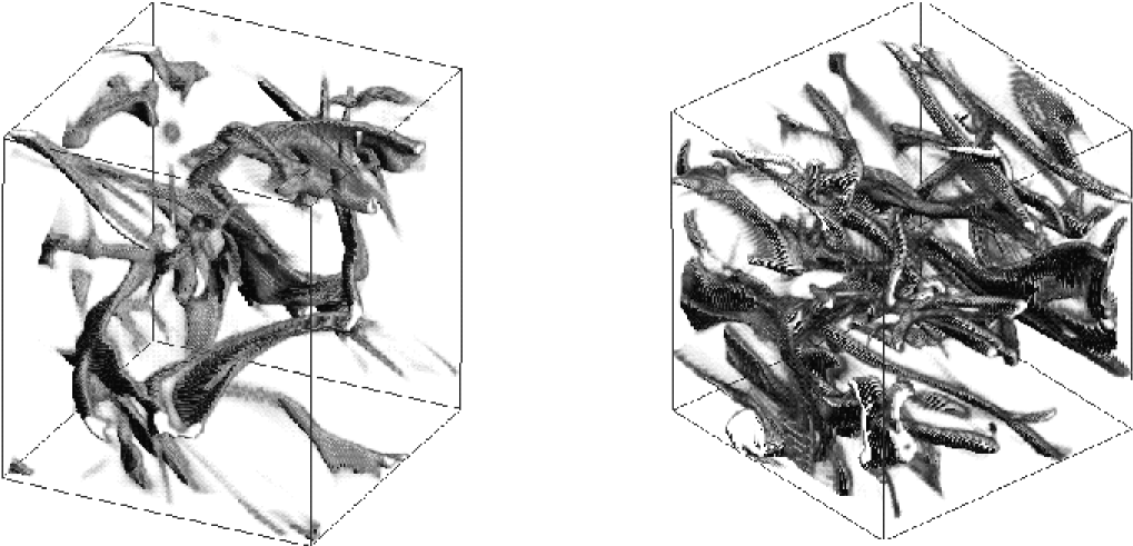
Figure 1:

Figure 2:

Figure 3:

Figure 4:

Figure 5:

Figure 6:

Figure 7:

Figure 8:

Figure 9:

Figure 10:

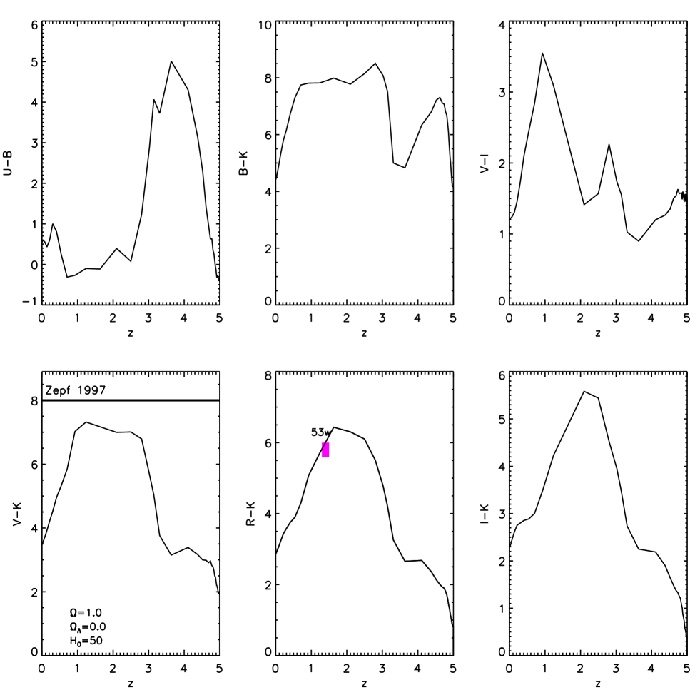
Figure 11:

Figure 12:

References

- (1) Aguirre A., Haiman Z., 1999. astro-ph, 9907039.
- (2) Blitz L., Shu F. H., 1980. ApJ, 238, 148.
- (3) Calzetti D., Kinney A. L., Storchi-Bergmann T., 1994. ApJ, 429, 582.
- (4) Calzetti D., 1997. AJ, 113, 162.
- (5) Caplan J., Ye T., Deharveng L., Turtle A., Kennicutt R., 1996. A&A, 307, 403.
- (6) Deharveng L., Caplan J., 1991. A&A, 259, 480.
- (7) Draine B. T., Lee H. M., 1984. ApJ, 285, 89.
- (8) Dunlop J., Peacock J., Spinrad H., Dey A., Jimenez R., Stern D., Windhorst R., 1996. Nature, 381, 581.
- (9) Dunlop J., 1997. astro-ph, 9704294.
- (10) Dunlop J., 1998. astro-ph, 9801114.
- (11) Elmegreen B. G., Lada C. J., 1977. ApJ, 214, 725.
- (12) Frayer D. T., Brown R. L., 1997. ApJSS, 113, 221.
- (13) Heavens A. F., Jimenez R., 1999. MNRAS, , in press.
- (14) Herbig G. H., 1962. ApJ, 135, 965.
- (15) Horner D. J., Lada E. A., Lada C. J., 1997. AJ, 113, 1788.
- (16) Hughes D. H., Serjeant S., Dunlop J., Rowan-Robinson M., Blain A., Mann R. G., Ivison R., Peacock J., Efstathiou A., Gear W., Oliver S., Lawrence A., Longair M., Goldschmidt P., Jenness T., 1998. Nature, 394, 241.
- (17) Jimenez R., Macdonald J., 1996. MNRAS, 283, 721.
- (18) Jimenez et al., 1998. astro-ph, 9812222.
- (19) Jimenez R., Padoan P., Matteucci F., Heavens A. F., 1998. MNRAS, 299, 123.
- (20) Jimenez R., Dunlop J., Padoan P., Peacock J., MacDonald J., Jorgensen U., 1999. MNRAS, in press.
- (21) Juvela M., 1997. A&A, 322, 943.
- (22) Kennicutt, Robert C. J., 1992. ApJSS, 79, 255.
- (23) Kennicutt R. C., 1998. ApJ, 498, 541.
- (24) Kurucz R., 1992. In: CDROM13.
- (25) Lada C. J., Gautier, T. N. I., 1982. ApJ, 261, 161.
- (26) Lada E. A., Lada C. J., 1995. AJ, 109, 1682.
- (27) Lada C. J., Alves J., Lada E. A., 1996. AJ, 111, 1964.
- (28) Lada E. A., Evans, Neal J. I., Depoy D. L., Gatley I., 1991. ApJ, 371, 171.
- (29) Lada C. J., Lada E. A., Clemens D. P., Bally J., 1994. ApJ, 429, 694.
- (30) Lada E. F., Lada E. A., Myers P. C., 1993. ApJ, 410, 168.
- (31) Lada C. J., Young E. T., Greene T. P., 1993. ApJ, 408, 471.
- (32) Leitherer et al., 1996. PASP, 108, 996.
- (33) Lowenthal J. D., Koo D. C., Guzman R., Gallego J., Phillips A. C., Faber S. M., Vogt N. P., Illingworth G. D., Gronwall C., 1997. ApJ, 481, 673.
- (34) Madau P., 1997. astro-ph, 9709147.
- (35) Maiz-Apellaniz et al., 1998. astro-ph, 9812138.
- (36) Mathis J. S., Rumpl W., Nordsieck K. H., 1977. ApJ, 217, 425.
- (37) Matteucci F., Ponzone R., Gibson B. K., 1998. A&A, 335, 855.
- (38) Mayya Y. D., Prabhu T. P., 1996. AJ, 111, 1252.
- (39) Meurer G. R., Heckman T. M., Calzetti D., 1999. ApJ, 521, 64.
- (40) Meyer D. M., Jura M., Hawkins I., Cardelli J. A., 1994. ApJL, 437, L59.
- (41) Padoan P., Nordlund A., 1999. ApJ, submitted.
- (42) Padoan P., Juvela M., Bally J., Nordlund Å., 1998. ApJ, 504, 300.
- (43) Padoan P., Bally J., Billawala Y., Juvela M., Nordlund A., 1999. ApJ, submitted.
- (44) Padoan P., Jimenez R., Jones B. J. T., 1997. MNRAS, 285, 711.
- (45) Padoan P., Nordlund Å., Jones B., 1997. ApJ, 474, 730.
- (46) Peacock et al., 1999. MNRAS, submitted.
- (47) Pettini et al., 1999. astro-ph, 9908007.
- (48) Pettini M., Kellogg M., Steidel C. C., Dickinson M., Adelberger K. L., Giavalisco M., 1998. ApJ, 508, 539.
- (49) Spinrad H., Dey A., Stern D., Dunlop J., Peacock J., Jimenez R., Windhorst R., 1997. ApJ, 484, 581.
- (50) Steidel et al., 1998. astro-ph, 9811399.
- (51) Steidel C. C., Pettini M., Hamilton D., 1995. AJ, 110, 2519.
- (52) Testor G., Niemela V., 1998. A&ASS, 130, 527.
- (53) Whitworth A., 1979. MNRAS, 186, 59.
- (54) Wilcots E. M., 1994. AJ, 107, 1338.
- (55) Williams R. E., Blacker B., Dickinson M., Dixon W. V. D., Ferguson H. C., Fruchter A. S., Giavalisco M., Gilliland R. L., Heyer I., Katsanis R., Levay Z., Lucas R. A., McElroy D. B., Petro L., Postman M., Adorf H.-M., Hook R., 1996. AJ, 112, 1335.
- (56) Xu C., De Zotti G., 1989. A&A, 225, 12.
- (57) Yoshii Y., Peterson B. A., 1994. ApJ, 436, 551.
- (58) Young J. S., Scoville N. Z., 1991. ARA&A, 29, 581.
- (59) Zepf S. E., 1997. Nature, 390, 377.