COBE and Global Topology: An Example of the Application of the Identified Circles Principle

Abstract

The significance to which the cosmic microwave background (CMB) observations by the satellite COBE can be used to refute a specific observationally based hypothesis for the global topology (3-manifold) of the Universe is investigated, by a new method of applying the principle of matched circle pairs.

Moreover, it is shown that this can be done without assuming Gaussian distributions for the density perturbation spectrum.

The Universe is assumed to correspond to a flat Friedmann-Lemaître model with a zero value of the cosmological constant. The 3-manifold is hypothesised to be a 2-torus in two directions, with a third axis larger than the horizon diameter. The positions and lengths of the axes are determined by the relative positions of the galaxy clusters Coma, RX J1347.5-1145 and CL 09104+4109, assumed to be multiple topological images of a single, physical cluster.

If the following two assumptions are valid: (i) that the error estimates in the COBE DMR data are accurate estimates of the total random plus systematic error; and (ii) that the temperature fluctuations are dominated by the naïve Sachs-Wolfe effect; then the distribution of the temperature differences between multiply imaged pixels is significantly wider than the uncertainty in the differences, and the candidate is rejected at the 94% level.

This result is valid for either the ‘subtracted’ or ‘combined’ Analysed Science Data Sets, for either $10^{\circ}$ or $20^{\circ}$ smoothing, and is slightly strengthened if suspected contaminated regions from the galactic centre and the Ophiuchus and Orion complexes are removed.

1 INTRODUCTION

1.1 Friedmann-Lemaître models: curvature and topology

At the end of last century, [][]Schw00,Schw98 dared to suggest ‘a few remarks’ which require ‘a total break with the astronomers’ deeply entrenched views’. He suggested (i) that geometers’ abstract concepts of non-Euclidean geometries could correspond to the real Universe, but also (ii) that non-trivial topology could also be required in order to represent the space in which we live. Since then, the physical theory (general relativity) linking his first suggestion, curvature, to the stress-energy tensor has encouraged considerable observational efforts in measuring (directly or indirectly) the curvature of the observable Universe.

On the other hand, mathematical difficulties and the lack of an accepted quantum gravity theory probably explain why less observational effort has been directed at following up the second of Schwarzschild’s two remarks that have ‘neither any real practical applicability nor any pertinent mathematical meaning’, i.e. measuring the topology of the Universe. Since the curvature estimates strongly favour a non-positive curvature, without measuring the topology of the Universe it is not possible to answer fundamental questions, such as whether or not the Universe is finite. (Measuring topology does not guarantee an answer, but not measuring it guarantees not having an answer, except if the curvature is positive.)

Both curvature and topology have been put in a relativistic context in the Friedmann-Lemaître models ([][]deSitt17,Fried24,Lemait58).

Mathematical developments in three-dimensional geometry and topology ([][]Thur82,Thur97) now abound, and theoretical ideas of the generation of topology at the quantum epoch are developing rapidly ([][]MadS97,Carl98,Ion98,DowS98,DowG98,Rosal98,eCF98,Gibb98,RatT98).

Recently, considerable work in observational methods, constraints and candidates for the global topology of the Universe has also commenced. These include (i) cosmic microwave background (CMB), i.e. essentially two-dimensional, methods (see SS1.2) and (ii) three-dimensional methods ([][]Fag87,Fag96,LLL96,Rouk96,RE97,Fag98,LLU98,RB98).

Work has also been done considering how simulations of large scale structure (the galaxy distribution) are affected by the usual assumption (for numerical rather than physical reasons) that the Universe is multiply connected ([][]FMel).

For theoretical reasons, interest is probably highest in the hyperbolic manifolds. However, the observational arguments tending towards a flat, cosmological constant dominated universe ([][]FYTY90,FortMD97,ChY97,SCP9812) may bring interest back to more thorough analyses of flat, multiply connected Friedmann-Lemaître models. Moreover, (i) for a cosmological constant to be observable, fine-tuning is necessary if an inflationary scenario is accepted, which may also fine-tune the topology scales such that ${r}_{\mbox{\rm\small inj}}<r_{\mbox{\rm\small SLS}}$; and (ii) the unknown physics required to explain $\lambda_{0}>0$ might also explain the topology of the Universe.

Hence, the flat models should not be neglected.

For reviews on cosmological topology, see [][]LaLu95,Lum98,Stark98 and [][]LR99.

The 2-D and 3-D methods have different underlying assumptions on the physics of regions of space or of objects, so systematic errors are likely to differ between the two approaches. Both have advantages and disadvantages. For a list and discussion of both 2-D and 3-D methods, see Table 2 of [][]LR99. A discussion restricted to the 2-D methods follows here.

1.2 Two-dimensional (CMB) methods for testing global topology

The 2-D methods cited above either (i) model (analytically or by simulations) the perturbation field in the universal covering space of compact universes and compare the random realisations (or statistics) with CMB data ([][]Stev93,Sok93,Star93,Fang93,JFang94,deOliv95,dOSS96,LevSS98a,BPS98) or (ii) analyse CMB data directly for multiple topological images (see SS2.2; [][]Corn96,Corn98b,Corn98a,Weeks98). [The method of [][]LevSS98b probably falls into the latter category, but is not discussed further.]

1.2.1 Advantages and disadvantages in the perturbation simulation approach

The fact that the former method (i), (which has been applied principally to Euclidean models, i.e. toroidal or hexagonal prismical models) makes statements about an ensemble of universe models can be interpreted as either an advantage or a disadvantage relative to the latter method (ii). The simulational methods (a) test consistency of observational and model perturbation statistics, based on (b) statistical properties of primordial perturbations, while the identified circles principle (SS2.2) directly tests whether or not the SLS is consistent with multiple topological imaging, using the actual temperature perturbations measured.

• The problem with a result about perturbation statistics is that the confidence level with which a particular multiply connected model can be rejected is only a statement about the rarity of perturbation properties required to be consistent with the observations.

  On the contrary, the circles principle enables rejection of a model by showing that temperatures at supposedly multiply topologically imaged points are inconsistent. That is, it can show that no set of perturbations would allow the model to fit the data.

• In addition, both theoretical and observational justification at large scales of the perturbation statistics assumed for the simulational approach are generally made under the assumption of simple connectedness. It could be considered inconsistent to test multiple connectedness if properties expected under the assumption of simple connectedness were assumed.

The theoretical motivations for Gaussian amplitude distributions and a $P(k)\propto k^{1}$ power spectrum are unlikely to be valid at scales approaching $2{r}_{\mbox{\rm\small inj}}$ and $r_{+}$.

That is, either for a hyperbolic or for a flat, $\lambda_{0}\sim 0.7$ metric to be presently observable (irrespective of topology), inflation needs some degree of fine-tuning [which can partly be provided by the ergodicity of geodesics in the former case, [][]Corn96]. For a flat, $\Omega_{0}=1$ multiply connected model to be observable, even more fine-tuning is needed.

So, either flat, observably multiply connected models can be rejected for purely theoretical reasons, or else they can be tested observationally accepting that perturbation statistics may differ somewhat from inflationary expectations.

Observational motivation for Gaussian amplitude distributions and a $P(k)\propto k^{1}$ power spectrum at the $2{r}_{\mbox{\rm\small inj}}$ and $r_{+}$ scales is equally lacking — if one is testing a multiply connected universe, since the only observational justification of these properties on large scales is that of COBE data analysed assuming simple-connectedness. Moreover, although several authors find consistency with Gaussian statistics (e.g. [][]Kogut95,Kogut96c,CollGP96), others find indications of non-Gaussianity ([][]Ferr98,Pando98), which are further discussed in [][]BrTeg99.

Apart from the problems inherent to the perturbation simulation approach, there are some factors which could be added to this approach but have not yet been dealt with in the work cited above dealing with flat multiply connected models:

• Only three of these eight papers discuss $T^{2}$ models, and only one compares such models with the COBE observations in any detail.

• The integrated Sachs-Wolfe effect (ISW) is not considered in any of the flat model papers. [Note that the ISW is discussed in [][]BPS98 for the hyperbolic case.]

• The possible contribution of redshifts in the SLS radiation due to peculiar velocities at the SLS (hereafter, ‘the Doppler effect’) is not considered in any of these papers. This is expected to contribute less than the naïve Sachs-Wolfe effect to temperature fluctuations $\delta T/T$ on COBE scales, under the assumption of simple-connectedness. However, if this assumption is dropped and ${r}_{\mbox{\rm\small inj}}<r_{\mbox{\rm\small SLS}}$ is being tested, it is difficult to be certain about properties of the velocity field on scales near ${r}_{\mbox{\rm\small inj}}$ based on present quantum cosmology theory.

  A conservative observational approach would be to consider statistics which take into account this locally anisotropic radiation.

• There is also a more local observational problem with the work done so far for flat and hyperbolic models. What is important for falsifying a small universe hypothesis is the significance of individual fluctuations, and whether or not these are multiply imaged.

  The significance of individual fluctuations has been studied by [][]CaySm95. This paper suggests that some of the most significant hot spots (above the 20 degree galactic cut) are galactic contaminants, from the Orion and Ophiuchus complexes. Removal of such non-axisymmetric contaminants has not yet been discussed in the small universe literature.

1.2.2 Advantages and disadvantages in the identified circles principle approach

Although tests based on the identified circles principle (SS2.2) avoid the problems (a) and (b) above, they share a weakness with the perturbation simulation approach by being adversely affected by noise, in particular from detector noise and from residual foreground contamination, which can make genuinely matched circles look different.

The ISW and Doppler effects will also provide some contributions to CMB maps. The former may be treated as foreground contamination. The latter will provide locally anisotropic emission, which should be taken into account as a modification of [][]Corn96’s identified circles principle (SS2.2.2).

The former is a weakness of applications of the identified circles principle, shared by the simulation approach, for non-flat models and models with a non-zero cosmological constant. The ISW, due to time varying of the gravitational potential, is likely to be strong if the Universe is hyperbolic, particularly at low redshifts and at the large angular scales present in the COBE maps ([][]Inoue99). In that case, temperature fluctuations at low redshifts are mixed in with the signal from the SLS, so that an identified circles analysis or a simulation analysis restricted to the SLS cannot account for the full signal at COBE scales.

1.2.3 Optimal comparison of multiply topologically imaged points

In view of the above comments, it is clear that for the testing of flat, small universe models, there are several advantages if the identified circles principle ([][]Corn96,Corn98b,Corn98a,Weeks98) can be used, since it avoids (a) making statistical statements about perturbations and (b) requiring assumptions about the statistics of the perturbations, even though it shares the problem of the perturbation simulation approach in its dependence on the statistics of detector noise and residual foregrounds.

There already exists a specific candidate for a small, flat universe which has been suggested by observations ([][]RE97,RB98). Because the candidate is fixed in astronomical coordinates, this offers a good example on which to see if COBE data can be used to reject a small universe hypothesis by using only the COBE data itself, without making theoretical hypotheses about the perturbation properties.

1.3 Observational rejection of [][]RE97’s (1997) $T^{2}$ candidate

The purpose of this paper is to see if this hypothesis, considered as a null hypothesis, can be rejected purely on the basis of the COBE observations, of about $\sim 300$ effectively independent pixels at which temperature fluctuations have been measured, without making assumptions regarding the statistics of primordial density perturbations.

1.3.1 The $T^{2}$ candidate

The candidate $T^{2}$ 3-manifold ([][]RE97,RB98), according to which two galaxy clusters at redshifts $z\sim 0.4$ would be topological images of the Coma cluster, is presented in SS2.1.

Apart from the striking fact that these three cluster images form a near right angle (in 3-D) and that right-angled ‘toroidal’ multiply connected universes are those which have been most extensively compared to observations, the relative simplicity of the hypothesis makes it ideal for testing if observational methods of refutation can really be made statistically watertight, in preparation for future candidate 3-manifolds, which are unlikely to be this simple.

Methods of refuting the supposed identity of the three clusters by their individual properties (positions and velocities of galaxies, overall masses, X-ray fluxes), by implied multiple imaging of large scale-structure, by predicted positions and redshifts of further topological images of the cluster and by proposals of observations relating to sub-cluster structures are discussed at length in SS4.2, SS4.3 and SS4.4 of [][]RBa99.

1.3.2 How to apply the identified circles principle to reject the $T^{2}$ candidate

The basic principle of any method used to constrain or detect candidates for the 3-manifold is that if the hypothesis of trivial topology is not adopted, then in some cases, photons can travel between a single, physical object or region of space to the observer by several different geodesics of (in general) widely differing lengths. That is, the objects or regions of space are observed at widely differing positions and redshifts.

In the case of the CMB, since the redshift is nearly equal for all points on the SLS by definition, only special subsets of angular positions on the SLS would be multiply imaged.

[][]Corn96,Corn98b realised that these special subsets form a well defined and easily described set in the covering space: the subsets are pairs of matched circles. The explanation for this is subtle, but elegant, and is briefly described in SS2.2.

If the radiation from the SLS is locally isotropic, then the observed temperature fluctuations observed around two circles of such a pair should be identical, to within the observational uncertainty.

If the values of corresponding points on the circles are inconsistent, then the hypothesis can be rejected with a confidence level based on the estimated uncertainty per resolution element, or pixel.

The assumption of local isotropy seems reasonable for the COBE data, due to the large smoothing length (effectively $10^{\circ}$). At this scale, the effective temperature correlations should be determined uniquely by the naïve Sachs-Wolfe effect ([][]SW67), i.e. by gravitational redshifts depending on the depths or heights of the potential wells.

As long as the gravitational potentials are spherically symmetric, i.e. if the equivalents of filaments and great walls on a linear scale do not exist at $z\sim 1100$, then this should be a fair assumption. If filaments and walls did exist, then since temperatures in two different COBE ‘pixels’ on corresponding circles represent averages over nearly two-dimensional spherical sections at different angles in the fundamental polyhedron, some modelling of the three-dimensional two-point correlation function would be needed in order to calculate the probability of these averages being identical.

For this paper, the averaging over the different spherical sections, each of diameter $\sim 1000$h^-1 Mpc (for $\Omega=1$) and $10^{\circ}$ smoothing, is assumed to result in identical values.

1.3.3 How to treat anisotropic (Doppler) radiation when applying the identified circles principle

The amplitude of the Doppler effect at the SLS, which is locally anisotropic, is assumed to be negligible relative to the naïve Sachs-Wolfe effect. Since the first Doppler ‘peak’ is on scales smaller than those resolved by the COBE DMR experiment, the fractional contribution of a Doppler component to an identified circles test of COBE data is probably small.

However, if ‘linear’ filaments and walls existed at the recombination epoch, or if velocity fields related to the ${r}_{\mbox{\rm\small inj}}$ scale existed, then this might not be correct.

It should also be remembered that the intrinsic spatial separations in a multiply connected universe can be much smaller in the fundamental polyhedron than in the covering space, so coherent velocity fields on apparently large, but inherently small, scales may generate a Doppler effect which would be unexpected under the simple connectedness assumption.

Although the naïve Sachs-Wolfe effect is assumed here to be dominant and to average out to locally isotropic values, an extension of [][]Corn98b’s (1998b) statistic which should be sensitive to Doppler dominated temperature fluctuations is suggested here, just in case the Doppler component is more important than expected.

If the Doppler effect dominates, then for pairs of multiply imaged pixels which also have nearly parallel lines-of-sight, the values should be nearly equal in absolute value, with equal signs if the angle between them is close to $0^{\circ}$ and opposite signs if the angle is close to $180^{\circ}$. Pixels for which the lines of sight are roughly orthogonal provide no theory-free constraint on topology if the Doppler effect is dominant.

Hence, a correlation function weighted by the dot product of the two line-of-sight vectors of each pixel pair should measure the degree to which the sets of points represent identical velocity induced temperature fluctuations. A dot product weighted correlation statistic is presented [eq. (4)] and demonstrated below.

1.4 Structure of paper and conventions

In SS2, the hypothesised 3-manifold is briefly presented (SS2.1), the matched circles principle is explained and the statistics used to estimate the consistency of multiply imaged ‘pixels’ on the CMB are defined (SS2.2), and the COBE data are briefly introduced (SS2.3). Results are presented in SS3 and discussed in SS4. Conclusions are in SS5.

The Hubble constant is parametrised here as $h\equiv H_{0}/100$km s^-1 Mpc${}^{-1}.$ Comoving coordinates are used (i.e. ‘proper distances’, [][]Wein72, equivalent to ‘conformal time’ if $c=1$). The metric assumed is flat, i.e., $\Omega_{0}+\lambda_{0}\equiv 1,$ since the candidate 3-manifold is $T^{2}\times R.$ The case $\lambda_{0}=0$ is the main case discussed here.

2 METHOD

2.1 The $T^{2}$ candidate

[][]RE97 pointed out that massive clusters of galaxies, dominated by their hot, X-ray emitting gas, should be relatively good ‘standard candles’ for observational constraints on the topology of the Universe. This was, in a sense, an update of the ‘classical’ searches for multiple topological images of single objects ([][]Gott80).

Although not a goal of that work, it was noticed that among a small number (seven) of very bright clusters used to illustrate the principle, three of these form nearly a right angle (to within $\sim 2-3$% depending on $\lambda_{0}$) with nearly equal (to 1%) arm lengths. This happens to be just what would be expected if space is $T^{3}$ with two side lengths equal and the third unknown, or if it is $T^{2}\times R.$ An a posteriori estimate of the probability of this occurring by chance is difficult to make in an unbiased way, so observational refutation is more prudent than theoretical refutation.

Moreover, this 3-manifold is very simple, relative to other flat 3-manifolds or to the hyperbolic 3-manifolds [which are considered more likely for several theoretical reasons, e.g. [][]Corn98a,eCF98]. The implied positions and redshifts of multiple topological images of objects are therefore relatively easy to calculate and observationally refutable predictions can be made. A list of the various observational arguments for and against the candidate, apart from the present study, is provided in the discussion section of [][]RBa99.

Table 1: The positions of the galaxy clusters Coma, CL 09104+4109 and RX J1347.5-1145 shown as J2000 right ascension ($\alpha$) and declination ($\delta$) in decimal degrees and redshift $z$. [Note: the label ‘J2000’ in Fig. 1 of [][]FabCr95 is interpreted as a typographical error for ‘B1950’.]

$$\begin{array}[]{l c c c}\hline\cr&\alpha&\delta&z\\ \hline\cr\mbox{Coma}&12.9969&27.9807&0.0239\\ \mbox{CL~{}09104+4109}&9.2289&40.9428&0.442\\ \mbox{RX~{}J1347.5-1145}&13.7918&-11.7533&0.451\\ \hline\cr\end{array}$$

The fundamental polyhedron (hereafter, FP) considered is therefore a nearly square, long prism. Two axes are defined as, $L_{x}{\bf e_{x}},$ the vector from the Coma cluster to the cluster CL 09104+4109 and $L_{y}{\bf e_{y}},$ the vector from the Coma cluster to the cluster RX J1347.5-1145. The third axis $L_{z}{\bf e_{z}}$ is defined as the cross product of these two vectors and assumed to be larger than the horizon diameter ($L_{z}>2R_{H}$). (The vectors ${\bf e_{x}},$ ${\bf e_{y}}$ and ${\bf e_{z}}$ are unit vectors.) The positions and redshifts adopted for the clusters are shown in Table 1.

The values of $L_{x}\approx L_{y}$ vary slightly from $\approx 960$h^-1 Mpc to $\approx 1230$h^-1 Mpc for $0\leq\lambda_{0}\leq 0{\cdot}9.$ $L_{z}$ is larger than the horizon diameter.

2.2 The Matched Circles Principle

Figure 1: Geometry in covering space showing how an observer sees multiple copies of circles on the CMB. Multiple copies of the observer which need to be considered are shown as black dots, and can labelled $(i,j)$ in units of the size of the Universe in the two small, fundamental directions. For clarity, the size of the Universe relative to the SLS (surface of last scattering) is larger than that of the candidate under consideration in this paper. The copy of the observer at $(0,1)$ is omitted for clarity. An image of the observer, for example, at $(3,1),$ is separated from the observer by a distance $\Delta$. The intersection of the SLS spheres of the two observers is a circle, of which two points lie in the plane of the figure. One such point is at A. Because the two observers are equivalent, the circle as seen by the observer at $(3,1)$ is equivalent to a circle seen in the same direction by the observer at the origin. That is, observer $(3,1)$ looking towards A is equivalent to observer $(0,0)$ looking towards A^′, and similarly for B and B^′. These two multiply imaged points in the plane are part of the the multiply imaged circle in three dimensions. The radius of the identified circles is $r_{ij}$. No identified circle is a great circle [except if $(0,0)$ were counted as a multiple image of the observer, which would not be useful]. The SLS has radius $r_{\mbox{\rm\small SLS}}.$ The dashed circle of radius $2r_{\mbox{\rm\small SLS}}$ is the maximum extent to which multiple images of the observer need to be considered.

The matched circles principle ([][]Corn98b) is illustrated in Fig. 1 and explained in this figure’s caption. Topological images of the observer in the lower half of the image are redundant (they give the same set of identified circles as the upper half). Depending on the value of the cosmological constant, $\lambda_{0},$ the ratio of $r_{\mbox{\rm\small SLS}}$ to $L_{x}\approx L_{y}$ for the $T^{2}$ candidate under consideration is $6.0\,\lower 2.58334pt\hbox{$\buildrel<\over{\sim}$}\,r_{\mbox{\rm\small SLS}}/L_{x}\,\lower 2.58334pt\hbox{$\buildrel<\over{\sim}$}\,13.2$ for $0\leq\lambda_{0}\leq 0{\cdot}9.$ This implies about three to six times as many circle pairs as shown in Fig. 1. Since some circles fall within or mostly within $20^{\circ}$ of the galactic plane, the number which can be usefully compared is smaller than this by about a third.

2.2.1 Locally Isotropic Radiation: the Sachs-Wolfe effect

To see if the measured temperature fluctuations are consistent with the hypothesis of physical identity of the circles, the most straightforward approach is to test the hypothesis that temperatures on corresponding pixels are equal to within observational error.

This hypothesis is tested here by considering the difference in the temperature fluctuations in two corresponding pixels on matched circles to be a random realisation of a Gaussian distribution centred on zero with a width determined by the uncertainties of the measurements in the two pixels. By normalising the distribution for each pair to have a standard deviation of unity, the full set of pairs of multiply imaged pixels can be combined to form a large sample of a single distribution of mean zero and standard deviation unity.

This standard deviation is $\sigma,$ defined

$$\sigma^{2}(r)\equiv\left<{\left[\left({\delta T\over T}\right)_{i}-\left({\delta T\over T}\right)_{j}\right]^{2}\over{\left[\Delta\left({\delta T\over T}\right)\right]_{i}^{2}+\left[\Delta\left({\delta T\over T}\right)\right]_{j}^{2}}}\right>.$$ (1)

where $\left({\delta T\over T}\right)_{i}$ and $\left({\delta T\over T}\right)_{j}$ are the temperature fluctuations in the two (hypothetically) multiple images of a single region of space-time.

The assumption that the mean difference is zero is likely to be a good approximation independently of whether or not the hypothesis is correct, since the dipole components have been subtracted off the data and little correlation should exist on such large scales if the assumption of simple-connectedness is correct. Nevertheless, it is useful to check the mean difference, which is defined

$$d\equiv\left<{\left({\delta T\over T}\right)_{i}-\left({\delta T\over T}\right)_{j}\over{\left\{\left[\Delta\left({\delta T\over T}\right)\right]_{i}^{2}+\left[\Delta\left({\delta T\over T}\right)\right]_{j}^{2}\right\}^{1/2}}}\right>.$$ (2)

It is also useful to consider the statistic of [][]Corn98b, which is essentially a two-point autocorrelation function normalised by the variance per pixel [eq. (2) of [][]Corn98b], though the interpretation is slightly less straightforward. This statistic is

$$S\equiv{\left<{2\left({\delta T\over T}\right)_{i}\left({\delta T\over T}\right)_{j}}\right>\over{\left<\left({\delta T\over T}\right)_{i}^{2}+\left({\delta T\over T}\right)_{j}^{2}\right>}}.$$ (3)

2.2.2 Doppler Effect

While it is possible that with the resolution of COBE, the Doppler effect averages out from three-dimensional space to the one-dimensional corresponding circles in a way which makes it negligible, the following variation on eq. (3) is proposed. This modified statistic is

$$S_{\mbox{\rm\small Dopp}}\equiv{{\left<2\left({\delta T\over T}\right)_{i}\left({\delta T\over T}\right)_{j}{\bf{\hat{n}}_{i}}{\boldmath.}{\bf{\hat{n}}_{j}}\right>}\over{\left<\left({\delta T\over T}\right)_{i}^{2}+\left({\delta T\over T}\right)_{j}^{2}\right>}}.$$ (4)

In a case where two corresponding pixels have orthogonal line-of-sight vectors, the two temperature values are unrelated (except if the three-dimensional centre of the pixel happens to be at the centre of a spherically symmetric gravitational potential), so a noise value would be contributed to $S$ [eq. 3], but nothing would be contributed to $S_{\mbox{\rm\small Dopp}}.$

In the case of corresponding pixels whose lines-of-sight are parallel and equal, contributions would be made both to $S$ and to $S_{\mbox{\rm\small Dopp}}.$ In the case of corresponding pixels whose lines-of-sight are parallel but opposite, a negative value (or anti-correlation) would be added to $S,$ but a positive value would be added to $S_{\mbox{\rm\small Dopp}}.$

For these reasons, if the Doppler effect (or another directional effect) were present (even partially), then the value of $S$ would be low and noisy in the presence of genuinely matched circles, to the extent to which the effect is present. On the other hand, $S_{\mbox{\rm\small Dopp}}$ would have a high value, although less than the ideal value of unity as would be expected for $S$ in the case of locally isotropic emission and a zero intrinsic (non-topological) auto-correlation function.

Table 2: Weights for the three frequencies of DMR measurements used for the ‘subtracted’ and ‘combined’ maps ([][]Bennett92,Bennett94).

$$\begin{array}[]{l c c c}\hline\cr&31\mbox{\rm GHz}&53\mbox{\rm GHz}&90\mbox{\rm GHz}\\ \hline\cr\mbox{subtracted}&-0.34&0.82&0.70\\ \mbox{combined}&-0.49&1.42&0.18\\ \hline\cr\end{array}$$

Although $S_{\mbox{\rm\small Dopp}}$ is calculated here out of interest, it is most likely to be useful in application to future measurements by the Planck and MAP satellites.

2.3 OBSERVATIONS

The COBE DMR observations and results are discussed by, for example, [][]Bennett94, in which a spherical harmonical analysis of the two year results is presented.

In this paper, the results of four years’ data are used, made available as ‘DMR Analysed Science Data Sets’ (hereafter, ASDS) by the COBE team, corrected for galactic emission either by the ‘subtraction’ or ‘combination’ techniques of removing synchrotron, dust and free-free emission. (Hereafter, the ‘subtracted’ and the ‘combined’ maps respectively.) The subtracted maps have the higher signal-to-noise ratio of the two. The weights for the three frequencies used to obtain the two maps (essentially those of [][]Bennett94) are listed in Table 2.

Because of galactic contamination, data between galactic latitudes of $-20^{\circ}$ and $+20^{\circ}$ are not considered.

Analysis of the significance of individual fluctuations (as opposed to their statistical significance) was carried out by [][]CaySm95. These authors noted (SS5 of [][]CaySm95) that some regions outside of the above galactic cut could also be galactic contaminants. The possibility that the second, third and seventh hot spots listed in Table 2B of [][]CaySm95 could be galactic contaminants due to the Ophiuchus complex and the Orion complex is considered here.

Since the data set is oversampled, a smoothing by a Gaussian of minimum full width half maximum (FWHM) of $10^{\circ}$ is necessary to extract a significant signal. In fact, as is shown below, the result is stronger if smoothing with a FWHM of $20^{\circ}$ is considered acceptable.

More recent analyses of galactic contamination of the DMR data have been discussed extensively by [][]Kogut96a,Kogut96b. Based on these discussions, alternative ways of combining the data from the six DMR antennae in order to further minimise galactic contamination relative to the ASDS maps provided by the COBE team, e.g. using a weighted average of the 53 and 90 GHz maps plus a ‘custom’ Galaxy cut, would be recommended for further applications of the circles principle using COBE data.

3 RESULTS

3.1 Difference parameters: $\sigma$ and $d$

Table 3: The values of the statistics $d,$ $\sigma,$ $S$ and $S_{\mbox{\rm\small Dopp}}$, as defined in eqs (2), (1), (3) and (4), for the COBE data.

$$\begin{array}[]{ c c c c}\hline\cr d&\sigma&S&S_{\mbox{\rm\small Dopp}}\\ \hline\cr\lx@intercol\mbox{`Subtracted' Analysed Science Data Set: }\hfil\lx@intercol\\ \lx@intercol\mbox{$10^{\circ}$ FWHM smoothing}\hfil\lx@intercol\\ -0.04&2.06&0.00&-0.01\\ \lx@intercol\mbox{$20^{\circ}$ FWHM smoothing}\hfil\lx@intercol\\ -0.20&2.71&-0.02&-0.01\\ \lx@intercol\mbox{`Combined' Analysed Science Data Set:}\hfil\lx@intercol\\ \lx@intercol\mbox{ 10${}^{\circ}$ FWHM smoothing }\hfil\lx@intercol\\ -0.01&1.54&0.02&-0.01\\ \lx@intercol\mbox{ 20${}^{\circ}$ FWHM smoothing }\hfil\lx@intercol\\ -0.14&1.93&0.02&-0.01\\ \lx@intercol\mbox{20${}^{\circ}$ FWHM; excluding G.C., Orion, Oph loop}\hfil\lx@intercol\\ -0.02&2.05&-0.03&-0.03\\ \hline\cr\end{array}$$

The values of the parameters representing pixel pair differences and correlations are listed in Table 3. Depending on whether the ‘subtracted’ ASDS or the ‘combined’ ASDS is used, and on whether smoothing is at the $10^{\circ}$ or the $20^{\circ}$ scale, the distributions of temperature differences in corresponding pixel pairs are clearly wider than the $\sigma=1$ distribution expected if the temperatures were intrinsically identical and the differences were only due to random measurement error.

Formally, a Kolmogorov-Smirnov test on the list of the normalised temperature differences used in calculating $\sigma$ and $d$ rejects the possibility that the distributions of these differences are drawn from a Gaussian distribution of mean zero and standard deviation unity by at least 94%. (The weakest rejection in Table 3 is for the ‘combined’ data set with $10^{\circ}$ smoothing; the other rejections are stronger.) This is the case whether or not the $N\sim 1000$ pixel pairs are considered to be independent, or whether only $\sim 150$ of these pairs (half the number of independent pixels) are considered to be independent. In either case, the large number of realisations of the difference distribution results in a precise value of the dispersion.

This result is only valid if the COBE team’s analysis of the random errors is correct, and if contributions from systematic errors are negligible. For example, if systematic errors or underestimates of the random errors caused the total uncertainties per pixel to be twice as high as the random uncertainties presented in the data set, then only the $20^{\circ}$ smoothed ‘subtracted’ data set would provide a significant contradiction.

Figure 2: Temperature fluctuations in COBE DMR data (the ‘combined’ four year Analysed Science Data Set, smoothed by $20^{\circ}$) around a selection of hypothetically identified circles in the CMB, modelled in the covering space, for $\Omega_{0}=1,$ $\lambda_{0}=0$, shown against the distance around each circle. Thick lines show the values $\delta T/T$ and thin lines show these values plus or minus the $1\sigma$ uncertainties. The horizontal length is the circle circumference. (By definition, no circles are great circles.) Each pair of circles is defined by the plane halfway between the observer and a topological image of the observer at $iL_{x}{\bf e_{x}}+jL_{y}{\bf e_{y}}$. The indexes $i$ and $j$ label each plot. The solid curves are for a circle at $(i,j)$ and the dashed curves for its matched circle at $(-i,-j).$ For the torus family of flat 3-manifolds, as in this case, the circles of a pair are parallel. The distance between the two members of a pair is therefore defined and is indicated here by $\Delta.$ Galactic latitudes between $-20^{\circ}$ and $20^{\circ}$ are excluded from the plots.

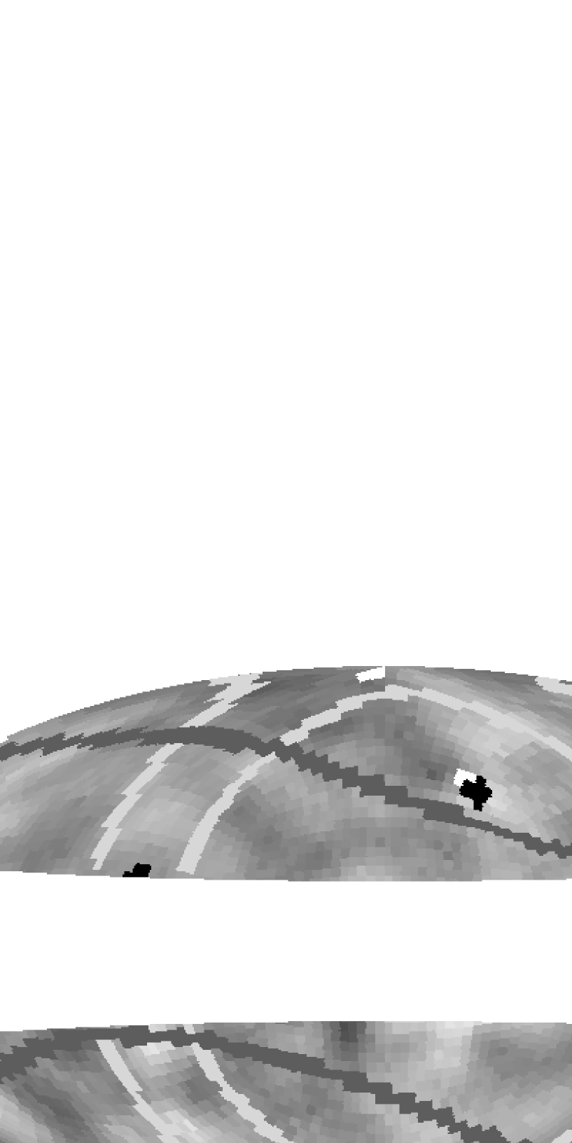
Figure 3: COBE DMR 10^∘ smoothed ‘combined’ ASDS map in Aitoff projection, with galactic latitude $b^{II}$ increasing from $-90^{\circ}$ to $90^{\circ}$ from bottom to top and galactic longitude $l^{II}$ decreasing from $180^{\circ}$ at the left to $-180^{\circ}$ at the right. A galactic cut of $\pm 20^{\circ}$ is applied. The positions of the three hypothesised fundamental axes determined by the three cluster images are indicated by black ‘spots’. From right to left, these are at $(-179^{\circ},41^{\circ})$, determined by the vector from Coma to CL 09104+4109, $(-35^{\circ},46^{\circ}),$ the vector from Coma to RX J1347.5-1145, and at $(75^{\circ},18^{\circ})$ the orthogonal third axis. The positions of the clusters (Sun centred observer) are shown by white ‘spots’: Coma is near the north galactic pole, the other two clusters are $\sim 3^{\circ}$ north of the corresponding axis directions. Identified circles for $(i,j)=(-2,2)$ and $(i,j)=(5,6)$ are shown as light and dark grey curves respectively (cf Fig. 2).

3.2 Matched circles

What are the actual values of the temperature fluctuations along the identified circles? Some examples of these are plotted in Fig. 2 and the positions of two large pairs of circles are shown in Fig. 3.

From this figure the reader can judge what typical fractions of the sky are available for comparison of matching circles, given the galactic cut of $\pm 20^{\circ}$ latitude and whether any systematic effects might be present.

Some of the pairs of circles look impressively similar.

Since the data is smoothed to $20^{\circ}\sim 2000$h^-1 Mpc, in the case of pairs of circles for which $\Delta<2000$h^-1 Mpc, it is clearly possible that some identity between corresponding circles can be induced just by the smoothing. For example, the temperature fluctuations around the two circles in the panel for $(i,j)=$ $(0,2)$ look very similar, but this is explainable by smoothing as much as by physical identity.

In the panels for $(-6,3),$ $(-5,2),$ $(-4,1)$ and $(-4,2)$ there are peaks which appear to coincide, though the overall slopes vary. In fact, these appear as much stronger, coinciding peaks in the ‘subtracted’ map. This suggests an explanation as a galactic feature. In other panels, such as $(-6,4),$ $(-6,5)$ $(-6,6)$ and $(-5,5)$ there are strong peaks which are highly in conflict between the two circles.

In the latter three cases, it could be argued that the temperature differences cannot be used to refute the $T^{2}$ candidate under consideration, because there could be contamination from the galactic centre, which may not have been subtracted perfectly, or may simply have left residual noise even if well subtracted. A large part of the central conflicting peaks in these three panels is indeed removed if an exclusion zone of $60^{\circ}$ around the galactic centre is applied.

Moreover, one could also remove areas possibly contaminated by the Ophiuchus complex and the Orion complex, as suggested by [][]CaySm95.

However, as can be seen statistically from the final three lines of Table 3, removal of areas possibly contaminated by the galactic centre and by the Ophiuchus and Orion complexes removes more well-matched parts of circles than ill-matched parts, with $\sigma$ increasing from $2.1$ to $2.4$ (the $\Omega_{0}=1,\lambda_{0}=0$ case is the one illustrated). For example, the central segments of panels for $(i,j)=$ $(4,6)$ and $(5,5)$ appear consistent within about $1\sigma,$ but both lie within $60^{\circ}$ of the galactic centre.

The positions of the Ophiuchus and Orion contaminations used are those listed as the second, third and seventh lines of Table 2B of [][]CaySm95. The radii of exclusion adopted are $57^{\circ},$ $9^{\circ}$ and $29^{\circ}$ respectively (based on the pixel numbers of the same table).

Examples of matching segments within $57^{\circ}$ of the first Ophiuchus component (and not within $60^{\circ}$ of the galactic centre) are the right-most segments in panels $(-3,3)$ and $(-1,6).$ Removal of these possible contaminating segments removes some conflicting segments, but also some consistent segments.

Finally, if one considers the panels which are least affected by the galactic cut, in particular panels $(-2,2),$ $(-1,1),$ $(5,6),$ $(6,5)$ and $(6,6),$ these seem to show little disagreement, apart from the right-hand end of the latter panels. Of these, the panel $(-1,1)$ is for a pair of circles only separated by $\Delta=1327$h^-1 Mpc, so the agreement can be explained by smoothing rather than by topology.

The right-hand end $(5,6),$ $(6,5)$ and $(6,6)$ can be removed to improve the agreement by arguing that this is contamination by the Ophiuchus complex, as before. However, this removal, and also removal of the galactic centre (as before) remove parts of the curves which do agree. If one takes the remaining parts of the curves, then there is still a broad agreement, for example if the data is further smoothed on a larger scale.

But in that case, there is the possibility that what matches is merely a quadrupole or dipole component which has been imperfectly subtracted. The dipole subtraction for the ASDS’s is quoted to be good but not perfect, so not only would a different statistic need to be calculated in order to measure the matching in such large scale gradients, but the dipole and quadrupole subtraction would have to be done precisely enough that this would be meaningful.

Figure 4: Dependence of $\sigma$, i.e. the standard deviation from identity of temperature fluctuations around hypothetically multiply imaged circles on the CMB, in units of the observational uncertainties [eq. (1)]. The value at galactic longitude $l^{II}=74.5^{\circ}$ is for the [][]RE97 $T^{2}$ cluster-based hypothesis and is clearly greater than $\sigma=1.$ Points at other longitudes are for other hypotheses equivalent to that of [][]RE97, except for a rotation in galactic longitude. The latter are unmotivated by observations. This and the following three figures are for the $20^{\circ}$ smoothed ‘combined’ map.

Figure 5: The mean temperature difference $d$ [eq. (2)] along identified circles is plotted, as for Fig. 4.

Figure 6: Dependence of $S$ [eq. (3)], the correlation statistic defined by [][]Corn98b, along identified circles as for Fig. 4.

Figure 7: Dependence of $S_{\mbox{\rm\small Dopp}}$ [eq. (4)], a modification of the $S$ statistic suggested for detecting correlations of the Doppler effect, along identified circles as for Fig. 4.

4 DISCUSSION

4.1 The $S$ statistic of [][]Corn98b

If the error estimates are correct, then the statistics above are sufficient to rule out the present $T^{2}$ hypothesis.

How successful is the correlation statistic $S$ of [][]Corn98b in refuting the candidate?

The values of $S$ shown in Table 3 are very low. Compared with Fig. 2 of [][]Corn98b, these values are quite surprisingly low. The details of the model for the figure are likely to differ somewhat from the present model, and the difference in using simulations versus observational data (in the present case) could explain some of the difference.

A value close to unity would be expected in an ideal case of matching circle pairs, and a value of zero for non-matching pairs, if the two-point auto-correlation function of the temperature fluctuations were zero. In reality, there is an intrinsic non-zero auto-correlation function, so a value showing this weak a correlation is unexpected.

If standard arguments implying the relative weakness of the Doppler effect are invalid, could this be due to a dominant contribution by the Doppler effect, which would cause genuinely anti-correlated temperature values to cancel when evaluating the $S$ statistic? The parameter $S_{\mbox{\rm\small Dopp}}$ does not support this. Its value is smaller in absolute value than that of $S$, presumably because typical values of ${\bf{\hat{n}}_{i}}{\boldmath.}{\bf{\hat{n}}_{j}}$ are smaller than unity and there is no underlying anti-correlation.

Figures 4-7 show that the small value of $S$ is just a coincidence. These plots show equivalent hypotheses to that based on the three clusters, apart from a rotation in galactic longitude. This avoids any systematic effects due to the galactic cut or to other functions of galactic latitude.

Assuming that the hypothesis is false, the ranges of values of the statistics for different longitudes show typical values of the parameters for the $T^{2}$ models equivalent to the hypothesised one (equivalent apart from the lack of observational motivation in the rotated models).

Fig. 6 shows why the low value of $S$ for the [][]RE97 candidate is just a coincidence. The position of the candidate just happens to lie at a longitude where both $d$ and $S$ have low (absolute) values. The longitudinal dependence of $d$ clearly has a sinusoidal-like component, which could be explained by some large scale feature in the temperature map. The longitudinal dependence of $S$ shows more complexity, and provides a distribution of maximum values about a factor of two to four times lower than those of ‘$S_{\mbox{\rm\small max}}$’ in [][]Corn98b’s simulation.

4.2 The $S_{\mbox{\rm\small Dopp}}$ statistic

The shape of the $S_{\mbox{\rm\small Dopp}}$ distribution (Fig. 7) is quite different from that of the $S$ distribution (Fig. 6). Typical values of $S_{\mbox{\rm\small Dopp}}$ are roughly half that of the typical $S$ values. An order of magnitude estimate to explain this is that (very) roughly half of the pairs of matched pixel vectors are roughly orthogonal, and so contribute very little to $S_{\mbox{\rm\small Dopp}}.$

Some features in the $S$ distribution, e.g. several local maxima and the global minimum in Fig. 6, can be identified with similar features in Fig. 7. These can be interpreted as features due to large matched circles for which the matched pixel vectors are roughly parallel.

Apart from the ‘missing’ contribution of orthogonal vectors in Fig. 7, the differences between the two figures also come from roughly opposite vector pairs, i.e. from pairs of small circles for large $i$ and $j$ values, where the ‘second observer’ is close to $2r_{\mbox{\rm\small SLS}}$ from the first observer.

This demonstrates an approach which will be particularly useful for the study of MAP and Planck Surveyor data. The statistic $S_{\mbox{\rm\small Dopp}}$ as defined in eq. (4) will provide a simple method of searching for roughly opposite, small identified circles in which a Doppler component is strongly expected to make a significant contribution.

If a candidate 3-manifold is detected in a new CMB map, then comparison of ‘false’ hypotheses rotated in galactic longitude such as here will provide a simple way of checking the significance of the detection, avoiding the need for simulations.

4.3 Comparison of COBE data to arbitrary $T^{2}$ models via simulated temperature fluctuations

In the absence of specific candidates for torus models, several authors have previously compared COBE data to sub-classes of these models, but using the perturbation simulational approach which requires assumptions on perturbation statistics as described above (SS1.2). The closest work among these to the present study is that of [][]dOSS96, who considered $T^{1}$ and $T^{2}$ models.

Because of the presence of one (or two) long axis(es), the ‘large-scale cutoff in Fourier mode’ argument for $T^{3}$ models, which can be valid for the assumptions of Gaussian random amplitudes in the Fourier modes, does not apply in these cases.

These authors defined a statistic, $S_{0},$ which is similar to $\sigma,$ but which includes multiply imaged pixel pairs along with many non-multiply imaged pixel pairs. The advantage of this is that the statistic is a minimum value, for which the orientation of the fundamental polyhedron is not assumed. The disadvantage is that non-multiply imaged pixel pairs are indiscriminately mixed with multiply imaged pixel pairs. The points (a), (b), (d), (e) and (f) (SS1.2.1) also apply to this study.

This enabled simulations, based on assumptions regarding the power spectrum of density perturbations, to be made in a parameter space comprising only the lengths of the fundamental polyhedron and two random variables for the Fourier modes, but not the orientation of the fundamental polyhedron. The statistic could therefore be calculated within practical computing capabilities.

Although this $S_{0}$ parameter is not identical to $\sigma,$ and it includes noise due to non-corresponding pixels, the value obtained is $2.59,$ not too much larger than the value of $\sigma$ which only compares matching pixels. This suggests that the $S_{0}$ parameter could still be useful for application to Planck and MAP data.

5 Conclusions

The COBE Advanced Science Data Sets (ASDS) have been used to try to refute the candidate for the global topology of the Universe defined by supposing that the three clusters Coma, RX J1347.5-1145 and CL 09104+4109 are three topological images of a single cluster and determine two generators of the 3-manifold, and that the third generator is large and orthogonal to the first two. The candidate is a $T^{2}\times R$ candidate, for a flat, i.e. $\Omega_{0}+\lambda_{0}=1$ universe, where $\lambda_{0}=0$.

Given the assumptions that

• the error estimates given in the ASDS’s are sufficient as good estimates of the total random plus systematic errors, and

• the temperature fluctuations measured are dominated by the naïve Sachs-Wolfe effect which averaged over spherical sections results in locally isotropic emission,

then,

• using either the ‘subtracted’ or the ‘combined’ ASDS,

• with smoothing at either $10^{\circ}$ or $20^{\circ}$, and

• with or without making cuts for possible contamination by the galactic centre and by the Ophiuchus and Orion complexes,

the difference statistics $\sigma$ and $d$ clearly refute the $T^{2}$ hypothesis to more than 94% significance. (This is estimated by a Kolmogorov-Smirnov test comparing the list of temperature differences to a Gaussian distribution of mean zero and standard deviation unity.)

A galactic cut of $\pm 20^{\circ}$ is used for all the above options.

The subtracted set more strongly rejects the hypothesis than the combined set. Smoothing at $20^{\circ}$ leads to a stronger rejection than for smoothing at $10^{\circ}.$ Removal of the suspected contaminating regions strengthens the rejection, suggesting that these introduce more spurious well-matched portions of circles than ill-matched portions.

This result does not rely on assumptions on the form of the fluctuation spectrum or on the distributions of amplitudes and phases of the spectrum.

The validity of assumption (i) will be tested by the increasingly numerous small angle measurements and by the Planck and MAP missions.

In the case of a non-zero cosmological constant ($\lambda_{0}=0,$ e.g. [][]FYTY90), the $T^{2}$ candidate has not yet been ruled out, since a modelling of the integrated Sachs-Wolfe (ISW) effect would be required. In this case, assumption (ii) would be invalid to the extent that the ISW contributes to the COBE CMB (SS7.3, [][]WSS94). If the magnitude of this component is of order of the estimated noise, then this would be equivalent to assumption (i) failing due to systematic error.

It is interesting to note that the matched circles principle provides a relatively clean and optimal method of refuting specific candidates for global topology. For data of the COBE quality, it is clear that there is strong sensitivity to the validity of the noise estimates. Since this is the case for the matched circles method, it must be an even stronger caveat for the perturbation simulation methods, which have mostly been applied to $T^{3}$ models for which $L_{x}=L_{y}=L_{z},$ for which the generators have been assumed to be mutually orthogonal, and for which simulations of the fluctuation spectra were required.

Since the effectiveness of this new method of applying the identified circles principle in order to directly refute a 3-manifold candidate (apart from the caveats) has been shown, future work would be to use the same method to refute certain classes of flat (or hyperbolic) multiply connected universe 3-manifolds with COBE data. This would complement previous work, which relied on assumptions on the perturbation statistics which are probably inconsistent with the hypotheses which were tested.

Bibliography

- [Bennett et al.(1992)] Bennett, C. L., et al., 1992, ApJ, 396, L7
- [Bennett et al.(1994)] Bennett, C. L., et al., 1994, ApJ, 436, 423
- [Bond(1996)] Bond J. R., 1996, in Cosmologie et structure à grande échelle, ed. Schaeffer R., Silk J., Spiro M., Zinn-Justin J., (Amsterdam: Elsevier), p475
- [Bond et al.(1998)Bond, Pogosyan & Souradeep] Bond J. R., Pogosyan D., Souradeep T., 1998, ClassQuantGra, 15, 2573 (astro-ph/9804041)
- [Bromley & Tegmark(1999)] Bromley B. C., Tegmark M., 1999, astro-ph/9904254
- [Carlip(1998)] Carlip S., 1998, ClassQuantGra, 15, 2629 (gr-qc/9710114)
- [Cayón & Smoot(1995)] Cayón L., Smoot G., 1995, ApJ, 452, 487
- [Chiba & Yoshii(1997)] Chiba M., Yoshii Y., 1997, ApJ, 489, 485
- [Colley et al.(1996)Colley, Gott & Park] Colley, W. N., Gott, J. R., Park, Ch., 1996, MNRAS, 281, L82
- [Cornish, Spergel & Starkman(1996)] Cornish N. J., Spergel D. N., Starkman G. D., 1997, gr-qc/9602039
- [Cornish, Spergel & Starkman(1998a)] Cornish N. J., Spergel D. N., Starkman G. D., 1998, Phys.Rev.D, 57, 5982 (astro-ph/9708225)
- [Cornish, Spergel & Starkman(1998b)] Cornish N. J., Spergel D. N., Starkman G. D., 1998b, ClassQuantGra, 15, 2657 (astro-ph/9801212)
- [de Oliveira Costa & Smoot(1995)] de Oliveira Costa A., Smoot G. F., 1995, ApJ, 448, 477
- [de Oliveira-Costa et al.(1996)de Oliveira-Costa, Smoot & Starobinsky] de Oliveira Costa A., Smoot G. F., Starobinsky A. A., 1996, ApJ, 468, 457
- [de Sitter(1917)] de Sitter W., 1917, MNRAS, 78, 3
- [Dowker & Garcia(1998)] Dowker H. F., Garcia R. S., 1998, ClassQuantGra, 15, 1859 (gr-qc/9711042)
- [Dowker & Surya(1998)] Dowker H. F., Surya S., 1998, PhysRevD, 58, 124019 (gr-qc/9711070)
- [e Costa & Fagundes(1998)] e Costa S. S., Fagundes H. V., 1998, gr-qc/9801066
- [Fabian & Crawford(1995)] Fabian A. C., Crawford C. S., 1995, MNRAS, 274, L63
- [Fagundes(1996)] Fagundes H. V., 1996, ApJ, 470, 43
- [Fagundes(1998)] Fagundes H. V., 1998, PhysLettA, 238, 235 (astro-ph/9704259)
- [Fagundes & Wichoski(1987)] Fagundes H. V., Wichoski U. F., 1987, ApJ, 322, L5
- [Fang(1993)] Fang, L.-Z., 1993, Mod.Phys.Lett.A, 8, 2615
- [Farrar & Melott(1990)] Farrar, K. & Melott, A.L., 1990, Computers in Physics, 4, 185
- [Ferreira et al.(1998)Ferreira, Magueijo & Gorski] Ferreira P. G., Magueijo J., Gorski, K. M., 1998, ApJ, 503, L1
- [Fort et al.(1997)] Fort B., Mellier Y., Dantel-Fort M., 1997, A&A, 321, 353
- [Friedmann(1924)] Friedmann A., 1924, Zeitschr.für Phys., 21, 326
- [Fukugita et al.(1990)] Fukugita, M., Yamashita, K., Takahara, F., Yoshii, Y., 1990, ApJ, 361, L1
- [Gibbons(1998)] Gibbons, G. W., 1998, ClassQuantGra, 15, 2605
- [Gott(1980)] Gott J. R., 1980, MNRAS, 193, 153
- [Inoue(1999)] Inoue, K. T., 1999, astro-ph/9810034
- [Ionicioiu(1998)] Ionicioiu R., 1998, gr-qc/9711069
- [Jing & Fang(1994)] Jing Y.-P., Fang L.-Z., 1994, PhysRevLett, 73, 1882 (astro-ph/9409072)
- [Kogut et al.(1996a)] Kogut, A., Banday, A. J., Bennett, C. L., Gorski, K. M., Hinshaw G., Reach W. T., 1996, ApJ, 460, 1
- [Kogut et al.(1996b)] Kogut, A., Banday, A. J., Bennett, C. L., Gorski, K. M., Hinshaw, G., Smoot, G. F., Wright, E. L., 1996, ApJ, 464, L5
- [Kogut et al.(1996c)] Kogut, A., Banday, A. J., Bennett, C. L., Gorski, K. M., Hinshaw, G., Smoot, G. F., Wright, E. L., 1996, ApJ, 464, L29
- [Kogut et al.(1995)] Kogut, A., Banday, A. J., Bennett, C. L., Hinshaw, G., Lubin, P. M., Smoot, G. F., 1995, ApJ, 439, L29
- [Lachièze-Rey & Luminet(1995)] Lachièze-Rey M., Luminet J.-P., 1995, PhysRep, 254, 136
- [Lehoucq et al.(1996)] Lehoucq R., Luminet J.-P., Lachièze-Rey M., 1996, A&A, 313, 339
- [Lehoucq et al.(1998)] Lehoucq R., Luminet J.-P., Uzan, J.-Ph., 1998, astro-ph/9811107
- [Lemaître(1958)] Lemaître G., 1958, in La Structure et l’Evolution de l’Univers, Onzième Conseil de Physique Solvay, ed. Stoops R., (Brussels: Stoops), p1
- [Levin et al.(1998a)Levin, Scannapieco & Silk] Levin J., Scannapieco E., Silk J., 1998a, Phys.Rev.D, 58, 103516 (astro-ph/9802021)
- [Levin et al.(1998b)Levin, Scannapieco & Silk] Levin J., Scannapieco E., Silk J., 1998b, ClassQuantGra, 15, 2689
- [Luminet(1998)] Luminet J.-P., 1998, gr-qc/9804006
- [Luminet & Roukema(1999)] Luminet J.-P., Roukema B. F., 1999, astro-ph/9901364
- [Madore & Saeger(1997)] Madore J., Saeger L. A., 1998, ClassQuantGra, 15, 811 (gr-qc/9708053)
- [Pando et al.(1998)Pando, Valls-Gabaud & Fang] Pando, J., Valls-Gabaud, D., Fang, L.-Zh., 1998, PhysRevLett, accepted, (astro-ph/9810165)
- [Peebles(1993)] Peebles, P.J.E., 1993, Principles of Physical Cosmology, Princeton, U.S.A.: Princeton Univ. Press
- [Perlmutter et al.(1999)] Perlmutter, S. et al., 1999, astro-ph/9812133
- [Ratcliffe & Tschantz(1998)] Ratcliffe, J. G., Tschantz, S. T., 1998, ClassQuantGra, 15, 2613
- [Rosales(1998)] Rosales J.-L., 1998, gr-qc/9712059
- [Roukema(1996)] Roukema B. F., 1996, MNRAS, 283, 1147
- [Roukema & Bajtlik(1999)] Roukema B. F., Bajtlik, S., 1999, MNRAS, in press, (astro-ph/9903038)
- [Roukema & Blanlœil(1998)] Roukema B. F., Blanlœil V., 1998, ClassQuantGra, 15, 2645 (astro-ph/9802083)
- [Roukema & Edge(1997)] Roukema B. F., Edge A. C., 1997, MNRAS, 292, 105
- [Sachs & Wolfe(1967)] Sachs, R. K., Wolfe A. M., 1967, ApJ, 147, 73
- [Schwarzschild(1900)] Schwarzschild, K., 1900, Vier.d.Astr.Gess., 35, 337
- [Schwarzschild(1998)] Schwarzschild, K., 1998, ClassQuantGra, 15, 2539 [English translation of Schwarzschild (1900)]
- [Sokolov(1993)] Sokolov, I. Yu., 1993, JETPLett, 57, 617
- [Starobinsky(1993)] Starobinsky A. A., 1993, JETPLett, 57, 622
- [Starkman(1998)] Starkman G. D., 1998, ClassQuantGra, 15, 2529
- [Stevens et al.(1993)] Stevens D., Scott D., Silk J., 1993, PhysRevLett, 71, 20
- [Thurston(1982)] Thurston, W. P., 1982, Bull.Am.Math.Soc., 6, 357
- [Thurston(1997)] Thurston, W. P., 1997, Three-Dimensional Geometry and Topology, ed. Levy, S., Princeton, U.S.A.: Princeton University Press
- [Weeks(1998)] Weeks J. R., 1998, ClassQuantGra, 15, 2599 (astro-ph/9802012)
- [Weinberg(1972)] Weinberg, S., 1972, Gravitation and Cosmology, New York, U.S.A.: Wiley
- [White et al.(1994)White, Scott & Silk] White, M., Scott, D., Silk, J., 1994, AnnRevA&A, 32, 319