The Amateur Sky Survey Mark III Project

Abstract

The Amateur Sky Survey (TASS) is a loose confederation of amateur and professional astronomers. We describe the design and construction of our Mark III system, a set of wide-field drift-scan CCD cameras which monitor the celestial equator down to thirteenth magnitude in several passbands. We explain the methods by which images are gathered, processed, and reduced into lists of stellar positions and magnitudes. Over the period October, 1996, to November, 1998, we compiled a large database of photometric measurements. One of our results is the tenxcat catalog, which contains measurements on the standard Johnson-Cousins system for 367,241 stars; it contains links to the light curves of these stars as well.

1 Introduction

In the year 1781, a musician and amateur astronomer named William Herschel discovered the planet Uranus while sweeping the skies with a homemade telescope in the back yard of his home in London. At that time, wealthy gentlemen could and did possess the equipment and knowledge to make significant advances in the science. During the next century, as astronomy evolved into a profession, academic and research institutions gradually dominated the field: only they possessed the resources to construct ever-larger telescopes and equip them with sophisticated instruments. Observatories moved to remote mountaintops in search of dark skies and good seeing, leaving the common man far behind. By the middle of the twentieth century, there were very few opportunities for amateur astronomers to contribute to the discipline: monitoring bright variable stars and atmospheric features of the planets, certainly, but little else.

In the past two decades, however, fortuitous developments in technology have given amateur astronomers a chance to rejoin the field. The combination of inexpensive CCD detectors and cheap, powerful computers permits any motivated individual to measure quantitatively the position and brightness of tens of millions of celestial sources. While the realm of the nebulae may still belong largely to the professional, the nearby universe is open to all.

In this paper, we describe a project in which we constructed our own equipment and used it to conduct a survey of bright stars near the celestial equator. Because most of us are amateurs, we call the project “The Amateur Sky Survey,” or “TASS” for short. After several experiments in designing celestial cameras (codenamed Mark 0 through Mark II), we settled on the Mark III device, which we describe in Section 2. In Section 3, we characterize the software used to reduce our images into lists of stars. We provide a few details on the observing locations (our back yards) in Section 4. We discovered that the really difficult part of this survey was keeping track of all the data (a common lesson in the current age of large-scale surveys), and so we devote Section 5 to the details of our solution. In Section 6 we discuss several results from the first three years of our work, and conclude in Section 7 by describing our future plans.

2 Hardware

The Mark III cameras were designed and constructed by one of us (TD) in 1995, then distributed gratis to observers across the country. We arrange our description of the subsystems to follow the order in which an incoming photon encounters them.

Each camera has an Aubell 135-mm f/2.8 camera lens. We chose this lens because it was on special at a New York camera store for $19, and was available in sufficient quantity to provide identical optics to all our units. We later noticed that while the lens gives reasonably sharp images (FWHM $\sim 23$ microns) in $V$-band, it performs poorly in $I$-band: the PSF shows a core surrounded by a halo, and its FWHM ($\sim 33$ microns) is considerably larger than that of the $V$-band PSF. We believe this inability to focus near-IR light accounts for most of the increased scatter in $I$-band photometry. Our future cameras will feature better optics.

Between the lens and the detector, we place filters manufactured to the Bessell (1990) prescription by Omega Optical, Inc. Each Mark III “triplet” contains three cameras mounted together (Figure 1). We usually chose two $I$-band and one $V$-band filters, but the Batavia triplet has one each of $V$, $R$ and $I$.

The heart of each camera is a Kodak KAF-0400 CCD detector. The KAF-0400 has 512 rows and 768 columns of $9$ micron pixels, with a full-well capacity of 85,000 electrons per pixel. We operate the CCDs in drift-scan mode: each chip is mounted so that its columns run east-west, parallel to the motion of stars across the sky. We read out the chip continuously, shifting charge along the columns at the same rate that stars drift across the detector. For a detailed description of drift-scanning, see Gehrels et al (1986). Our 135-mm lens yields a plate scale of about $13.8$ arcseconds per pixel; the effective exposure time is the time required for a star to drift $512\times 13.8{\rm\ arcsec}\sim 1.96$ degrees on the equator: 471 seconds.

The length of our exposures requires us to cool the CCD well below ambient temperatures. Each CCD is attached to a two-stage thermoelectric (TE) cooler: the first stage does most of the work, dropping the temperature by about $30^{\circ}$ Celsius. The second stage is driven by a circuit which acts to maintain the temperature at a constant value. We place a large bucket of water next to the triplet at each site to act as a heat sink at roughly constant temperature, and circulate the water through the TE coolers. Although the water may cool down during the course of a night by a large amount, the temperature regulation can hold the CCD at a temperature constant to within $\sim 0.01^{\circ}$ C.

The specifications of the Kodak KAF-0400 show a read noise of 13 electrons. When running our cameras at a typical operating temperature of $-15^{\circ}$ Celsius, we measure a total noise of 25 to 30 electrons in dark images. Photon noise from the sky at our sites overwhelms the readout and thermal noise: the total noise ranges from 50 to 120 electrons per pixel in a $V$-band image, and from 90 to 150 electrons in an $I$-band image.

Three cameras are bundled together in each triplet (see Figure 1). The body holds the cameras in a common plane, but points them at 15-degree intervals. We set the triplets to point near the celestial equator, with one camera looking on the meridian (due south), one looking an hour to the east, the third looking an hour to the west. A star may drift through all three cameras during a single night. We built a single electronics board, located in the back of the triplet housing, to control all three cameras. For simplicity’s sake, we used a single clock driver to time the control signals to all three CCDs. The camera operator at each site tuned the driver by trial and error to achieve the best setting. We discovered that the single driver was a mistake: small variations in the focal lengths of the cameras made it impossible to optimize the PSF in all three simultaneously.

Each camera produces a long, continuous image of the night sky, about three degrees wide from north to south and as long as the night is clear. The electronics board within the triplet housing sends the data, one row at a time, over a byte parallel line to a nearby computer. The computer reads the information and writes it to disk in 16-bit integer FITS format, breaking the stream of pixels into images of roughly 900 rows (about 3.5 degrees in Right Ascension).

3 Observations

Since the Mark III cameras require power, cooling water, and a computer, as well as manual intervention to cover them from the elements, we placed them in our backyards; the camera operators have day jobs and cannot drive long distances to dark sites on a daily basis. Operation consists of uncovering the cameras at dusk and starting a computer program. The operator then leaves the unit alone, just making sure to cover up the camera before it rains or the sun shines into the lens. In the morning, the data files are processed to star lists when time is available.

The data presented herein were taken at three suburban sites: near Cincinnati, Ohio, longitude 84.58 West, latitude 39.20 North, operated by MG; near Dayton, Ohio, longitude 83.87 West, latitude 39.80 North, operated by GG; and near Batavia, Illinois, longitude 88.33 West, latitude 41.83 North, operated by TD. A fourth triplet at the Applied Physics Lab of Johns Hopkins University, longitude 76.88 West, latitude 39.15 North, has also run regularly.

The weather at these sites is poor, especially in the winter months: our coverage of the equator is weakest between 6 and 12 hours Right Ascension. Even when the weather is good, we are sometimes unable to collect data due to other commitments. As a result, over the roughly two years from October, 1996, to November, 1998, the three sites combined to submit measurements from 175 nights. Obviously, we could increase the data rate by a factor of two to four by placing a triplet within a weather-proof housing at a site with good weather and automating its operation. We plan to put the first of our next generation of instruments in Arizona for exactly this reason.

The skies of our suburban locations are much brighter than those at most observatories. On a typical night in Batavia, the sky brightness is about eighteenth magnitude per square arcsecond in both $V$-band and $I$-band. At a dark site ($\sim 21.0$ mag/square arcsecond in $V$), the noise background due to sky brightness would decrease by a factor of about four, which would increase our limiting magnitude by a bit more than one magnitude.

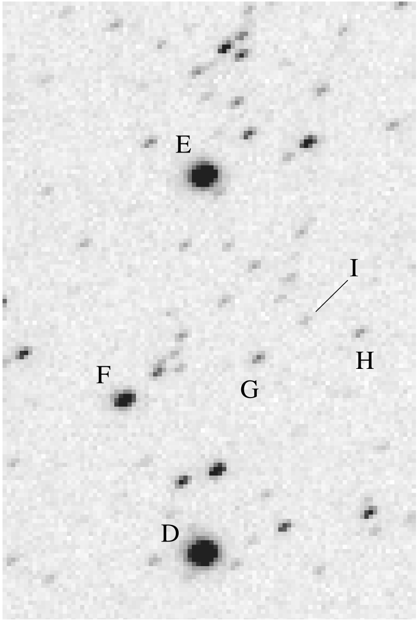
Figure 3: Closeup of the dashed box in Figure 2. Star F = HD 67769 ($V=9.4$), G = GSC 4847-02290 ($V=12.0$), H = GSC 4847-02482 ($V=12.4$), I = GSC 4847-02614 ($V=13.2$). North is up and East to the left.

During an eight-hour night, each camera scans roughly 360 square degrees. The images are stored on disk and processed into star lists the next day. Depending on the season and sky brightness, a triplet may record 50,000 to 200,000 measurements on a good night. Most sources are detected two or three times, at one-hour intervals. Our images provide good data for sources from seventh magnitude to thirteenth or fourteeth magnitude. We provide an example of a $V$-band Mark III image in Figure 2: it shows a field roughly 4 degrees wide by 3 degrees high at the intersection of Monoceros, Canis Minor, and Hydra. Figure 3 shows a closeup view of the area bounded by the dashed box in Figure 2; note the slightly diagonal shape of the PSF.

4 Software

We have written all the software used to record the image data, clean the images, detect and measure stellar sources. In each step, we follow standard procedures and employ conventional algorithms; nonetheless, we describe our pipeline in some detail so that readers may understand the limitations it places on the final results.

4.1 Cleaning the raw images

Since we take drift-scan images, the signal from each star passes through every row along one column of the CCD. Correcting the images requires the construction and application of one-dimensional dark and flatfield vectors.

We make a dark vector for each camera on each night by taking an image of several hundred rows with the lens cap in place, then calculating the median of the pixel values in each column.

We create a flatfield vector in a slightly different manner. In order to improve the signal-to-noise ratio, we start with scans taken during twilight. First, we subtract the dark vector from the scans. Now, since the brightness level changes rapidly at these times, we cannot simply take the median of several hundred rows as a fair measure of the change in sensitivity across the chip. Therefore we calculate the flatfield vector in two steps. First, we create a set of temporary flatfield vectors, one for each row in our twilight image, by dividing the pixel values in that row by the median pixel value of that row. We then create a single flatfield vector whose column values are the median value of each column from our set of temporary flat vectors.

We normalize the flatfield vector and then divide each dark-subtracted raw image by it.

4.2 Generating a PSF

For each frame, we first calculate the sky value and the standard deviation from that value. Next, we find all sources with peaks at least 20 times the standard deviation above the sky. To make a quick estimate of the Full Width at Half-Maximum (FWHM) of the PSF, we walk down from the peak pixel along the rows and columns until the pixel value drops to half that of the peak. We use the median value of this rough FWHM in the row and column directions as a first approximation.

We make a second pass through the sources, discarding any with FWHM values which deviate from the first approximations by more than $25\%$. We calculate the average FWHM in each direction from the remaining peaks. We then create a bounding rectangle whose width and height are 2.55 times the average FWHM (i.e. 3 sigma for a true gaussian) in each direction. We create a set of PSF’s by normalizing each peak within the bounding rectangle. We average all the PSF’s in the set to determine the final PSF. We therefore have a strictly empirical PSF for each image.

We build an “optimized aperture” from this discrete PSF by selecting whole pixels, working outwards from the center, until the next pixel value drops to less than one-fourth of the average pixel value included so far. This aperture has the same shape as the PSF, but discards pixels in which the signal-to-noise of a star is low.

4.3 Finding stars

Following DAOPHOT (Stetson 1987), we convolve the image with a lowered PSF to detect sources. We mark as a candidate peaks in the convolved image above a threshold (typically two or three times the standard deviation from the sky). We measure the sky-subtracted flux of the candidate in the original image through the optimized aperture, and use it to calculate the ratio

$$f={\rm{flux\ inside\ aperture}\over{\rm{peak\ in\ convolved\ image}}}$$

A true star has a value of $f$ close to 1.0, while cosmic rays and other spurious detections typically yield very different values. We accept any candidate with $f$ within a reasonable range of the expected value.

4.4 Measuring stellar properties

To calculate the position of each detected star, we use pixels within the aperture to form marginal sums in the row (column) directions. We add the sums for each row (column) to form a cumulative marginal sum, then interpolate to find the row (column) at which the sum reaches half its final value. Our interpolation scheme yields positions which are fractions of a pixel.

We convert the (row, col) position of each star into (RA, Dec) by matching the brightest 30 stars in each image against stars in the Tycho catalog (ESA 1997); we have adapted the triangle-based method described by Groth (1986) and Valdes et al. (1995) to match the detected and catalog positions of the stars. Each detection is tagged with the time at which it passed the midpoint of the field of view, based on its position within the image and the time at which the image was read from the camera.

To calculate the flux of each detected star, we do not use this interpolated position. Instead, we adopt the position of the peak in the image convolved with the PSF. At this position in the original image we place the “optimized aperture,” and add (flux - sky) contributed by each pixel within the aperture. We estimate an uncertainty in each measurement by combining contributions from readout noise, sky subtraction, and photon noise from the source itself.

4.5 Photometric calibration

Each Mark III camera converts instrumental magnitudes to the standard Johnson-Cousins system via a two-step calibration procedure.

First, in order to set a preliminary zero-point for the instrumental magnitudes, we consider a particular subset of stars from the Tycho catalog. We choose stars which

• are not marked as variable in the Tycho catalog,

• have $B_{T}$ and $V_{T}$ uncertainties of $\leq 0.06$ mag,

• are fainter than $V_{T}=7.5$ so that they are not saturated,

• are separated from other Tycho stars by at least 83 arcsec in RA and 50 arcsec in Dec.

Since the TASS cameras observe in Johnson-Cousins $VRI$, we need to convert the Tycho $B_{T}$ and $V_{T}$ magnitudes to the Johnson-Cousins system. We found a set of 300 Tycho stars brighter than $V=9$ which matched Landolt ( 1983, 1992) standards. We performed linear fits to $V,R,$ and $I$ versus $(B_{T}-V_{T})$, finding transformation equations:

$$V = \phantom{-}0.0156+V_{T}-0.0994(B_{T}-V_{T})$$ (1)

$$R = -0.0160+V_{T}-0.5390(B_{T}-V_{T})$$ (2)

$$I = -0.0468+V_{T}-0.9480(B_{T}-V_{T})$$ (3)

Note that the V equation is similar to that given in the Hipparcos (ESA 1997) catalog:

$$V = V_{T}-0.090(B_{T}-V_{T})$$ (4)

but with slightly different coefficients. To ensure uniformity, we adopted the new coefficients. Note also that each of these equations is only valid over a limited color range, and the quality of the fit degrades as one moves further from the $B_{T}$ passband. We have therefore further restricted the Tycho subset to stars within the color range of $-0.2<(B_{T}-V_{T})<2.0$.

We then compare these approximate Johnson-Cousins magnitudes to our instrumental magnitudes for the same stars in our images; we simply shift the instrumental magnitudes by a constant to match the catalog values. This procedure places our observations on the standard Johnson-Cousins system without having to make separate observations of Landolt fields (often impossible for cameras scanning a few degrees from the celestial equator), and makes use of non-photometric nights since the Tycho reference stars are contained within each image.

After a year or so of operation, we discovered that cameras at several sites exhibited small, systematic errors in photometry as a function of Declination. Apparently, the one-dimensional flatfield vectors we create do not perfectly remove variations in response across the field of view. Fortunately, the errors are nearly constant over the course of a single night. We correct them by breaking the three-degree Declination range of each camera into a small number (typically 8) of zones. In each zone, we make a linear fit to the (observed - expected) residuals as a function of Declination, using Tycho stars from the entire night; we force the corrections to agree at each boundary between zones. We then add these corrections to the magnitude of all stars observed on that night. This Declination-dependent correction reduces the residuals of repeated measurements of bright stars in the $V$-band from about 55 millimagnitudes to about 35 millimagnitudes.

The results of this two-step procedure are stored locally by each site and made available for further analysis. We have detected small color terms in these measurements from some of the Mark III cameras at some of the sites; see the discussion on color corrections in the tenxcat catalog in Section 6.2.

5 Database

There have been three to four Mark III triplets active at any time over the past three years. During a typical night of operation, a single triplet measures over 100,000 stellar positions and magnitudes. Keeping track of the data generated at all sites is not a trivial task.

The operator of each triplet is responsible for processing the data into “star lists:” ASCII tables of stellar positions and magnitudes, with a small amount of ancillary information. Each operator periodically sends accumulated star lists via FTP, ZIP disks or CDs, to one of our members (MR) who acts as DataBase Manager (DBM). The DBM occasionally loads the star lists into our central database. In no sense is this a real-time operation: the interval between observation and insertion into the database varies from weeks to months.

We have adopted the PostgreSQL database engine for our project: it is a relational database with an SQL syntax which runs on many platforms and is distributed free of charge. One of us (CA) designed the tables required to hold the information generated by each site, and the software necessary to load the information into the database. The central database runs on the desktop computer in the DBM’s office, where it competes for disk space and memory with many other projects. The information from roughly 175 nights of observation requires about 5 Gigabytes of disk space.

Once the data has been loaded into the database, it may be analyzed in many ways. Users from any computer with an SQL client and an Internet connection can access the information freely. We have built WWW interfaces to service common queries so that novice users need only a web browser to answer simple questions.

One of the main functions of the database is to identify measurements of the same star in different images, so that one can calculate mean values or look for variability. We wrote software to perform this merging of data with the following method in mind: if a new detection appears more than $D$ arcseconds from any existing entry in the database, consider it a new entity; but if it appears within $D$ arcseconds of an existing entry, mark it as an additional observation of the existing entry. We chose $D=15$ arcseconds, based on the precision of our measurements of position (see below) and on the large size of our pixels.

We seeded the database with stars from the USNO A1.0 catalog (Monet 1996) down to sixteenth magnitude, to serve as initial, accurate positions. Our plan was to keep the USNO A1.0 position as the database position until a star was recorded some large number $N$ times; then we would switch to using the star’s mean observed position. In this way, random errors in the first few recorded measurements would not cause the position to wander by large amounts (several arcseconds), but, eventually, the database would contain a position based on our measurements alone. Unfortunately, we made an error in our software, setting $N=1$; thus, the position for each star in our database did wander by significant amounts. In some cases, the database position moved so far from the true position that a new measurement did not fall within $D=15$ arcseconds of the existing position; the new measurement was then recorded (incorrectly) in the database as an independent star. We estimate that perhaps 5 percent of all stars in our database suffer from this “spurious companion” problem; we provide one post facto fix in our discussion of the tenxcat catalog, below.

6 Results

We are still exploring the wealth of information garnered during two years of operation, and several sites are still contributing new observations. The items mentioned below are simply the first projects to which we have put our energies; many avenues of study await the curious researcher. For example, we have not yet tried to perform any search for objects which move in the sky from one night to the next.

In one sense, the primary result of our work cannot be presented in this paper: it is the database of measurements we have collected. This database continues to grow as we incorporate new observations from several sites. There is no restriction on access to the data; TASS members and non-members alike may sift through it on an equal basis. We encourage readers who have a use for the information to visit the WWW pages which describe database access.

6.1 Precision of Astrometry and Photometry

The Mark III cameras do not provide precise positions. The telephoto lens and CCD yield a plate scale of about $13.8$ arcseconds per pixel, the PSF is often asymmetric, and the $I$-band PSF features an extended halo. Comparing the position of a single TASS measurement for a bright star to the position listed in the Hubble Guide Star Catalog (Lasker et al 1990), we find a scatter of about 3 arcseconds; the scatter rises to about 6 arcseconds near our detection limit. The mean of many measurements is considerably more accurate; see Section 6.2 below.

The photometric measurements produced at each camera site and transmitted to the central database may suffer from systematic color terms (see discussion in tenxcat section below). We ignore that source of error here, and consider only the precision of the measurement: as a metric, we use the standard deviation from the mean of measurements of the same star by the same camera on many different nights. We find that the standard deviation from the mean has a minimum of about 0.03 mag for bright stars, increasing to more than 0.20 mag for stars near the limits of detection.

If one calculates the expected uncertainty in photometric measurements, using measured values for readout noise and estimates of the sky brightness, one finds much smaller values. The Mark III measurements are evidently not limited by photon noise, except for the very faintest stars. The major sources of error are imperfect sky subtraction and variations in the PSF across our field of view.

Since we measure most stars many times, the mean values of our measurements should provide information on each star more precise than that from a single observation. We therefore have constructed a catalog which contains the mean values of position and magnitude for stars observed multiple times.

6.2 The tenxcat Catalog

After two years of operation, the total number of detections reported to the central database reached more than 10 million in $V$, 0.7 million in $R$, and 13 million in $I$. However, many of these detections were due to noise peaks, airplane trails, cosmic rays, and other contaminants. In order to generate a catalog of reliable celestial sources, we selected objects in the database which appeared on at least 10 different occasions, in any combination of passbands. We call this the tenxcat catalog: it contains 367,241 stars at the time of writing (September, 1999). Interested readers can access the catalog via the Internet at

http://www.tass-survey.org/tass/www_scripts/make_chart.html

We subjected the objects in this subset to two additional steps of processing.

• We checked each of the Mark III cameras for color terms, by comparing their measurements of equatorial standard stars against those of Landolt ( 1983; 1992). The $R$-band and $I$-band cameras had statistically significant residuals as a function of stellar color, which we list in the Appendix. We therefore applied linear corrections to the TASS magnitudes from those cameras to bring their measurements to the Johnson-Cousins magnitude scale.

• We checked each star for “spurious companions:” neighbors within $D=15$ arcseconds which never appear in the same image as the star, and have the same brightness to within 0.5 mag. Whenever possible, we merged such pairs of stars into a single entry in our database, and marked the remaining entry with a flag.

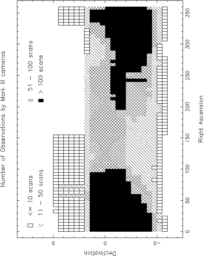
Figure 4: Number of observations by Mark III cameras as a function of position on the sky.

We are constrained by our drift-scan cameras to observe near the celestial equator: our surveyed area described a rough band from Declination $=-5^{\circ}$ to $1.5^{\circ}$. We emphasize that this is by no means a complete catalog; as Figure 4 shows, the number of observations varies considerably throughout our survey area. Since some faint stars were not detected in all images, an area would need to covered many more than 10 times for all its stars to be included in tenxcat.

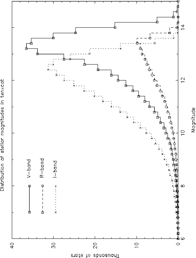
Figure 5: Distribution of magnitudes for stars in the tenxcat catalog.

The tenxcat catalog contains stars ranging from about seventh magnitude to about fourteenth magnitude. However, the distribution of stellar magnitudes (Figure 5) shows that the number of stars per magnitude bin begins to fall at about $V=13.3$, $R=13.3$, $I=12.5$. The difference between the passbands is a combination of the color of a typical star and the system sensitivity as a function of wavelength.

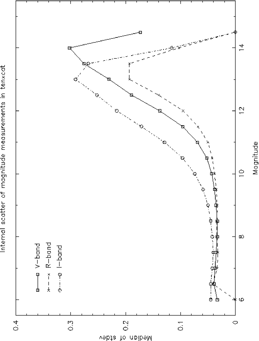
Figure 6: Median values of standard deviation from the mean for magnitudes of stars in the tenxcat catalog.

The internal consistency of our photometric measurements can be gauged by calculating the median value of the standard deviation from the mean within magnitude bins. In Figure 6 we show the results for all 3 passbands; all three have a floor of about $\sigma=0.04$ mag, but the scatter increases much more quickly in $I$ band than in $V$ or $R$. We blame the $I$-band results on three factors: first, the $I$-band images suffered from a core-halo PSF; second, we combined $I$-band measurements from 5 different cameras at 3 different sites, whereas there were only 3 different cameras with $V$ filters and a single camera with $R$ band filter; third, our photometric calibration in $I$ depends upon extrapolation in the transformation from Tycho $B_{T},V_{T}$ to Johnson-Cousins $I$ (see the Appendix).

The positions in tenxcat are the mean values from at least 10 different measurements. We have compared our positions against those in the ACT Reference Catalog (Urban et al 1998) to judge the accuracy of the mean positions. We find the median difference between TASS and ACT positions to rise slowly with magnitude, from $0.59$ arcseconds at $V=7.5$ to $0.89$ arcseconds at $V=11.5$. The mean positions of fainter stars are less accurate, but still good to a few arcseconds.

In order to facilitate the identification of sources, we include cross-references between stars in tenxcat and other catalogs. Each entry in our catalog has a field for the matching entry in the Hubble Guide Star Catalog (Lasker et al 1990) and the ACT Reference Catalog (Urban et al 1998). We have extracted from the ACT Reference Catalog information from the Henry Draper (HD) catalog (Cannon & Pickering 1918-1924; Cannon 1925), including the spectral type; unfortunately, tenxcat contains only 7792 stars with data from the HD. Finally, we have compared the position of each of our stars against sources in the IRAS Point Source Catalog (Beichman et al 1988); any star which falls within 20 arcseconds of an IRAS source is marked with the IRAS identifier.

The catalog is available as an ASCII text file, and via a WWW form which allows the user to search through it in several ways. A detailed description of each field in the catalog, and instructions on accessing it electronically, are provided in Richmond ( 1999b).

6.3 Variable Stars

One of the strengths of the Mark III survey is the number of times it has scanned some areas of the sky. Recall that two of our sites have two $I$-band cameras on their triplets, providing measurements of each star roughly two hours apart during a single night. In addition, we have spent many nights observing the celestial equator during the past few years. As a result, of the 367,241 stars in tenxcat, over 16,000 have at least 30 measurements in $V$-band and over 55,000 have at least 30 measurements in $I$-band. We have arranged our database so that remote users may easily retrieve all observations of one particular star, or generate a light curve on the fly.

One obvious use for this wealth of data is to study variable stars. We describe here several different ways in which our members have started to mine the database.

Gombert ( 1998a; 1998c; 1999) has searched for variable stars which do not appear in existing catalogs, finding over 60 candidates. He finds that the Mark III data is especially well-suited to finding Mira-like variables: one can isolate stars with large $(V-I)$ colors and examine several years of observations. Gutzwiller ( 1999) has found another 52 candidates. These efforts are by no means an exhaustive search of the entire Mark III dataset, but will keep us busy gathering followup observations (for an example, see Dvorak 1999).

While our positions are not as accurate as those in astrometric catalogs, they are certainly better than many listed in the General Catalog of Variable Stars (GCVS) (Kholopov et al 1992). When the identity of a variable in the GCVS is uncertain, due to a poor position, one can examine the light curve of all stars in the vicinity in our database and often find the variable easily. Gombert ( 1998b) provides positions accurate to a few arcseconds for 51 known variable stars.

Our archives do not include images of the sky, only measurements of position and brightness for the sources we detect. The Stardial project (McCullough & Thakkar 1997), on the other hand, does save all of its images, but doesn’t perform any source detection or measurement. Since the Mark III and Stardial surveys share a very large area on the sky (about 1400 square degrees in a strip from Dec = $0^{\circ}$ to $-4^{\circ}$), one can combine them to find objects which would not stand out in either survey alone. Hassforther and Bastian ( 1999) have found a Mira variable by searching visually a set of Stardial images; although the star disappears from Stardial at minimum light, it is still detected in our $I$-band measurements. We expect to see many other projects combine the Mark III data with information from other sources.

7 Future Work

The Mark III survey will continue for several years. We have already gathered several seasons of data from a fourth site (the Applied Physics Lab at Johns Hopkins) to be incorporated into the database. This paper represents only a “snapshot” of a working project; we may export several updated versions of our catalog(s) before reaching the final version.

TASS members have shifted most of their attention and efforts away from the Mark III survey to a new project: the Mark IV systems. A Mark IV unit will consist of two cameras fixed side-by-side on a common mount; each camera combines a 100mm f/4 lens, a single filter, and a Lockheed/Fairchild 442A CCD with $2048\times 2048$ pixels to provide a field of view four degrees on a side. The mount allows motion in Hour Angle and Declination, and is designed to track accurately for several minutes. We estimate the detection limit of the system to be fainter than fifteenth magnitude. We are currently constructing seven Mark IV systems, the first of which will be deployed at Flagstaff in Fall 1999.

Appendix A Appendix

There were 23 cameras built and distributed for the Mark III survey. Of these, 16 are known to have operated and to have taken at least some data. Twelve have been operated almost every clear night at their locations. Data from 9 cameras is presently included in database:

• 3 V-band cameras, one at each site

• 1 R-band camera, at Batavia

• 5 I-band cameras: 2 each at Dayton and Cincinnati, 1 at Batavia

We compared TASS measurements of stars against Landolt’s equatorial catalogs of UBVRI standard stars (Landolt 1983; 1992). The V-band measurements showed no significant offset in the mean, nor any significant color dependence. We therefore made no correction to the V-band measurements. In the R and I bands, however, there were both small offsets in the mean (always in the sense that TASS measurements were slightly fainter than Landolt measurements), and small trends in residuals as a function of (V-I) color. See TASS Technical Note 54 (Richmond 1999a) for details, graphs, and tables.

We determined the following color terms, based on stars brighter than mag 11 and using a color which was the mean TASS V value (based on measurements from all cameras) minus the mean TASS I value (based on measurements from all cameras). In the equations below, uppercase values represent corrected single magnitude measurements, and lowercase values represent raw single magnitude measurements.

$$R-band$$

$${\rm camera\ H1\ (Batavia):\ }R =r+0.01209-0.073704*(color)$$

$$I-band$$

$${\rm camera\ B0\ (Dayton):\ }I =i-0.0563-0.018676*(color)$$

$${\rm camera\ B2\ (Dayton):\ }I =i-0.0683+0.040971*(color)$$

$${\rm camera\ D0\ (Cinn):\ }I =i-0.0844+0.06116*(color)$$

$${\rm camera\ D2\ (Cinn):\ }I =i-0.1001+0.08510*(color)$$

$${\rm camera\ H2\ (Batavia):\ }I =i+0.0121-0.073704*(color)$$

After making the corrections to each individual measurement, we then re-calculated the mean magnitude of each star in all passbands. In cases of spurious pairs, we made the corrections to each member of the pair separately, based on its own color, re-calculated mean magnitudes for each member separately, and finally determined a weighted mean magnitude for the merged entity.

The corrected tenxcat magnitudes agree well with Landolt magnitudes, with little dependence on color.

Figure 1: A Mark III triplet, seen from the back (North) side. The lens has been removed from the East camera. The plastic tubing circulates cooling water through each camera.

Figure 2: Mark III $V$-band image of the area near (J2000) RA = 08:09:45, Dec = -01:06:30, covering 4 degrees E-W by 3 degrees N-S. Star A = HD 66950, B = HD 68667, C = HD 67111, D = HD 67720, E = HD 67719. North is up and East to the left.

References

- (1) Beichman, C. A., Neugebauer, G., Habing, H. J., Clegg, P. E., & Chester, T. J. 1988, IRAS Catalogs and Atlases, Version 2. Explanatory Supplement, NASA Ref. Publ. 1190
- (2) Bessell, M. S. 1990, PASP, 102, 1181
- (3) Cannon, A. J. & Pickering, E. C. 1918-1925, The Henry Draper Catalogue, Ann. Astron. Obs. Harvard College, 91-99
- (4) Cannon, A. J. 1925, The Henry Draper Extension, Ann. Astron. Obs. Harvard College, 100, 17
- (5) Dvorak, S. 1999, http://home.att.net/ RollingHillsObs
- (6) Gehrels, T., Marsden, B. G., McMillan, R. S. & Scotti, J. V. 1986, AJ, 91, 1242
- (7) Gombert, G. 1998a, Inf. Bull. Var. Stars, 4575
- (8) Gombert, G. 1998b, Inf. Bull. Var. Stars, 4609
- (9) Gombert, G. 1998c, Inf. Bull. Var. Stars, 4653
- (10) Gombert, G. 1999, Inf. Bull. Var. Stars, 4709
- (11) Groth, E. J. 1986, AJ, 91, 1244
- (12) Hassforther, B. & Bastian, U. 1999, Inf. Bull. Var. Stars, 4742
- (13) ESA 1997, Hipparcos and Tycho Catalogues, ESA SP-1200, 1, 57
- (14) Kholopov, P. N., Samus, N. N., Durlevich, O. V., Kazarovets, E. V., Kireeva, N. N., & Tsvetkova, T. M. 1992, Bull. Inf. Centre Donnees Stellaires, 40, 15
- (15) Lasker, B. M., Sturch, C. R., McLean, B. J., Russell, J. L., Jenkner, H., & Shara, M. M. 1990, AJ, 99, 2019
- (16) Landolt, A. U. 1983, AJ, 88, 439
- (17) Landolt, A. U. 1992, AJ, 104, 340
- (18) McCullough, P., & Thakkar, U. 1997, PASP, 109, 1264
- (19) Monet, D. 1996, USNO A-1.0: a catalog of astrometric standards (Washington, DC: USNO)
- (20) Richmond, M. W. 1999a, TASS Technical Note 54, http://www.tass-survey.org/tass/technotes/tn0054.html
- (21) Richmond, M. W. 1999b, TASS Technical Note 56, http://www.tass-survey.org/tass/technotes/tn0056.html
- (22) Stetson, P. B. 1987, PASP, 99, 191
- (23) Urban, S. E., Corbin, T. E., Wycoff, G. L., Martin, J. C., Jackson, E. S., Zacharias, M. I. & Hall, D. M. 1998, AJ, 115, 1212
- (24) Valdes, F. G., Campusano, L. E., Velasquez, J. D., & Stetson, P. B. 1995, AJ, 107, 1119
- (25)