[

Reconstructing the Cosmic Equation of State from Supernova distances

Abstract

Observations of high-redshift supernovae indicate that the universe is accelerating. Here we present a model-independent method for estimating the form of the potential $V(\phi)$ of the scalar field driving this acceleration, and the associated equation of state $w_{\phi}$. Our method is based on a versatile analytical form for the luminosity distance $D_{L}$, optimized to fit observed distances to distant supernovae and differentiated to yield $V(\phi)$ and $w_{\phi}$. Our results favor $w_{\phi}\simeq-1$ at the present epoch, steadily increasing with redshift. A cosmological constant is consistent with our results.

]

The observed relation between luminosity distance and redshift for extragalactic Type Ia Supernovae (SNe) appears to favor an accelerating Universe, where almost two-thirds of the critical energy density may be in the form of a component with negative pressure [2, 3, 4, 5, 6]. Although this is consistent with $\Omega_{\rm M}<1$ and a cosmological constant $\Lambda>0$ (e.g. [7]), at the theoretical level a constant $\Lambda$ runs into serious difficulties, since the present value of $\Lambda$ is $\sim$10¹²³ times smaller than predicted by most particle physics models[8].

However, neither the present data nor the theoretical models require $\Lambda$ to be exactly constant. To explore the possibility that the $\Lambda$-like term (e.g. quintessence) is time-dependent, we use a model for it that mimics the simplest variant of the inflationary scenario of the early Universe. A variable $\Lambda$-term is described in terms of an effective scalar field (referred to here as the $\Lambda$-field) with some self-interaction $V(\phi)$, which is minimally coupled to the gravitational field and has little or no coupling to other known physical fields. In analogy to the inflationary scenario, more fundamental theories like supergravity or the M-theory can provide a number of possible candidates for the $\Lambda$-field but do not uniquely predict its potential $V(\phi)$. On the other hand, it is remarkable that $V(\phi)$ may be directly reconstructed from present-day cosmological observations.

The aim of the present letter is to go from observations to theory, i.e. from $D_{L}(z)$ to $V(\phi)$, following the prescription outlined by Starobinsky [9] (see also [10]). This is the first attempt at reconstructing $V(\phi)$ from real observational data without resorting to specific models (e.g. cosmological constant, quintessence etc.).

Since the spatially flat Universe ($\Omega_{\phi}\!+\!\Omega_{\rm M}\!=\!1$) is both predicted by the simplest inflationary models and agrees well with observational evidence, we will not consider spatially curved Friedmann-Robertson-Walker (FRW) cosmological models. In a flat FRW cosmology, the luminosity distance $D_{L}$ and the coordinate distance $r$ to an object at redshift $z$ are simply related as ($c=1$ here and elsewhere)

$$a_{0}r=a_{0}\int_{t}^{t_{0}}\frac{dt^{\prime}}{a(t^{\prime})}=\frac{D_{L}(z)}{1+z}.$$ (1)

This uniquely defines the Hubble parameter

$$H(z)\equiv\frac{\dot{a}}{a}=\left[\frac{d}{dz}\left(\frac{D_{L}(z)}{1+z}\right)\right]^{-1}.$$ (2)

Note that this relation is purely kinematic and depends neither upon a microscopic model of matter, including a $\Lambda$-term, nor on a dynamical theory of gravity.

For a sample of objects (in this case, extragalactic SNe Ia) for which luminosity distances $D_{L}$ are measured, one can fit an analytical form to $D_{L}$ as a function of $z$, and then estimate $H(z)$ from (2). If $\rho_{m}=(3H_{0}^{2}/8\pi G)\Omega_{\rm M}(a/a_{0})^{-3}$ is the density of dust-like cold dark matter and the usual baryonic matter, then

$$H^{2} = \frac{8}{3}\pi G\left(\rho_{m}+{1\over 2}\dot{\phi}^{2}+V(\phi)\right),$$ (3)

from where it follows that

$$\dot{H}=-4\pi\,G(\rho_{m}+\dot{\phi}^{2}).$$ (4)

Eqs. (3) & (4) can be rephrased in the following form convenient for our current reconstruction exercise,

$${8\pi G\over 3H_{0}^{2}}V(x)\ = {H^{2}\over H_{0}^{2}}-{x\over 6H_{0}^{2}}{dH^{2}\over dx}-{1\over 2}\Omega_{\rm M}\,x^{3},$$ (5)

$${8\pi G\over 3H_{0}^{2}}\left({d\phi\over dx}\right)^{2} = {2\over 3H_{0}^{2}x}{d\ln H\over dx}-{\Omega_{\rm M}x\over H^{2}},$$ (6)

where $x\equiv 1+z$. Thus from the luminosity distance $D_{L}$, both $H(z)$ and $dH(z)/dz$ can be unambiguously calculated. This allows us to reconstruct the potential $V(z)$ and $d\phi/dz$ if the value of $\Omega_{M}$ is additionally given. Integrating the latter equation, we can determine $\phi(z)$ (to within an additive constant) and, therefore, reconstruct the form of $V(\phi)$. Note also that the present Hubble constant $H_{0}\equiv H(z\!=\!0)$ enters in a multiplicative way in all expressions. Thus, neither the potential $V(\phi)/H_{0}^{2}$ nor the cosmic equation of state $w_{\phi}(z)$ depends upon the actual value of $H_{0}$.

FIG. 1.: The maximum deviation $\Delta D_{L}/D_{L}$ between the actual value and that calculated from the ansatz (7) in the redshift range $z=$0–10, as a function of $\Omega_{\rm M}\equiv 1-\Omega_{\phi}$. The three curves plotted are for constant values of the equation of state parameter (as defined in Eq. 12) $w_{\phi}=-1$ (solid line), $-2/3$ (dotted line) and $-1/3$ (dashed line).

A fitting function for $D_{L}$: We use a rational (in terms of $\sqrt{x}$) ansatz for the luminosity distance $D_{L}$,

$${D_{L}\over x}\equiv\frac{2}{H_{0}}\left[\frac{x-\alpha\sqrt{x}-1+\alpha}{\beta x+\gamma\sqrt{x}+2-\alpha-\beta-\gamma}\right]$$ (7)

where $\alpha$, $\beta$ and $\gamma$ are fitting parameters. This function has the following important features: it is valid for a wide range of models, and it is exactly equal to the analytical form given by (1) for the two extreme cases: $\Omega_{\phi}=0,1$. At these two limits, as $\Omega_{\rm M}\to 1$, $\alpha+\gamma\to 1$ and $\beta\to 1$ ; and as $\Omega_{\rm M}\to 0$, $\alpha,\beta,\gamma\to 0$. The accuracy of our ansatz is illustrated in Fig. 1.

We choose this form since the value of $H(z)$ obtained by differentiating $D_{L}/x$, according to (2), has the correct asymptotic behavior: $H(z)/H_{0}\to 1$ as $z\to 0$, and $H(z)/H_{0}=\tilde{\Omega}_{\rm M}^{1/2}(1+z)^{3/2}$ for $z\gg 1$, where

$$\tilde{\Omega}_{\rm M}=\left({\beta^{2}\over\alpha\beta+\gamma}\right)^{2}.$$ (8)

This ensures that at high-$z$, the Universe has gone through a matter dominated phase. It should be noted that $\tilde{\Omega}_{\rm M}$ can be slightly larger than the CDM component $\Omega_{\rm M}$ since the $\Lambda$-field (or quintessence) can have an equation of state mimicking cold matter (dust) at high redshifts. For instance, $\tilde{\Omega}_{\rm M}\simeq 1.1\,\Omega_{\rm M}$ in the quintessence model considered by Sahni & Wang [11]. On the other hand, $\tilde{\Omega}_{\rm M}\mathrel{\hbox to0.0pt{\lower 3.0pt\hbox{$\mathchar 536\relax$}\hss}\raise 2.0pt\hbox{$\mathchar 316\relax$}}1.15\,\Omega_{\rm M}$, to ensure that there is sufficient growth of perturbations during the matter-dominated epoch (see, e.g., the relevant discussion in [9]).

Note that the right hand side of (6) should be non-negative for the minimally coupled scalar field model. At $z=0$, this condition gives

$${{4\beta+2\gamma-\alpha}\over{2-\alpha}}\geq 3\Omega_{\rm M},$$ (9)

where the equality sign occurs when the $\Lambda$-term is constant. The fact that $D_{L}$ is smaller in a universe with time-dependent $\Lambda$-term than it is in a constant-$\Lambda$ universe leads to a lower limit for the parameter $\beta$. When taken together with the fact that $\beta\to 1$ as $\Omega_{\rm M}\to 1$ ($\Omega_{\phi}\to 0$) this leads to the following set of constraints

$$1\leq\frac{1}{\beta}\leq\frac{1}{2}\int_{1}^{\infty}{dx\over\sqrt{1-\Omega_{\rm M}+\Omega_{\rm M}x^{3}}}.$$ (10)

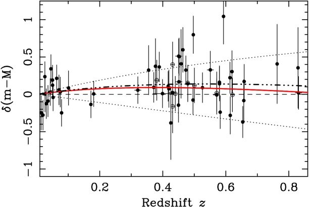
FIG. 2.: The distance modulus $(m-M)$ of the SNe Ia relative to an $\Omega_{\rm M}\to 0$ Milne Universe (dashed line), together with the best-fit model of our ansatz (7), plotted as the solid line. The extreme cases of the ($\Omega_{\rm M}$, $\Omega_{\phi}$)= (0, 1) and (1, 0) universes are plotted as dotted lines. Also plotted as the dot-dashed line is the best fit Perlmutter et al. [2] model ($\Omega_{\rm M}$, $\Omega_{\phi}$)= (0.28, 0.72). The filled circles are the 54 SNe of the “primary fit” of [2]. The high-$z$ SNe of [3] (not used in this analysis) are plotted as open circles.

The observational data: Till date, about 100 SNe Ia in the redshift range $z\!=0.1\!-\!1$ have been discovered, a large fraction of which have reliable published data from which luminosity distances can be calculated. We use the 54 SNe Ia from the preferred “primary fit” (‘C’ in their Table 1) of the Supernova Cosmology Project [2], including the low-$z$ Calan Tololo sample [12] as used therein. We adopt the quoted redshifts, reducing them to the cosmic microwave background frame.

TABLE I.: Best-fit parameters

$\Omega_{\rm M}=$		0.2	0.25	0.3
$\alpha=$		$1.702^{+0.191}_{-0.518}$	$1.630^{+0.209}_{-0.539}$	$1.533^{+0.229}_{-0.575}$
$\beta=$		$0.585^{+0.019}_{-0.020}$	$0.604^{+0.022}_{-0.023}$	$0.615^{+0.025}_{-0.027}$
$\gamma=$		$-0.230^{+0.043}_{-0.045}$	$-0.255^{+0.048}_{-0.052}$	$-0.252^{+0.056}_{-0.061}$
$\kappa=$		$1.226\pm 0.018$	$1.229\pm 0.018$	$1.232\pm 0.018$
$\langle\chi^{2}\rangle$=		1.03	1.03	1.03	a
$\tilde{\Omega}_{\rm M}$=		$0.2\pm 0.11$	$0.25\pm 0.16$	$0.3\pm 0.23$

Maximum likelihood fits: The luminosity distance $D_{L}$ (Mpc) is related to the measured quantity, the corrected apparent peak $B$ magnitude $m_{B}$ as $m_{B}=M_{0}+25+5\,\log_{10}D_{L}$, where $M_{0}$ is the absolute peak luminosity of the SN. The function to be minimized is

$$\chi^{2}\equiv\sum_{i=1}^{n}\frac{\left[y(z_{i})-y(m_{Bi})\right]^{2}}{\sigma_{i}^{2}};\ ~{}y(z)\equiv 10^{M_{0}/5}D_{L}(z).$$ (11)

A fourth fitting parameter, $\kappa=2\times 10^{M_{0}/5}(c/H_{0})$, which is required in addition to $\alpha,\beta,\gamma$ in the above minimization process, includes both $M_{0}$ and $H_{0}$, which cannot be measured independent of each other. For instance, if $M_{0}\!=\!-19.5\pm 0.1$ and $\Omega_{\rm M}\!=\!0.3$, the value of $H_{0}\!=\!61.3\pm 2.9$ km s^-1 Mpc^-1. Note that $\kappa$ only features in the fit of (7) to the data, and does not play a role in the reconstruction of $V(\phi)$.

To obtain the best fit model, we perform an orthogonal chi-square fit, using errors on both the magnitude and redshift axes in $\sigma_{i}$, subject to the constraints (9), (10) and the condition $\tilde{\Omega}_{\rm M}\simeq\Omega_{\rm M}$. The latter condition is used for simplicity – our results remain essentially the same even if we use the entire permitted range $\tilde{\Omega}_{\rm M}\mathrel{\hbox to0.0pt{\lower 3.0pt\hbox{$\mathchar 536\relax$}\hss}\raise 2.0pt\hbox{$\mathchar 316\relax$}}1.15\,\Omega_{\rm M}$.

The results shown in Table I and in Figure 2 are for $\Omega_{\rm M}=0.3$. In arriving at the best fit, the two constraints in (10) are found to be redundant, which means that only two constraints, (9) and $\tilde{\Omega}_{\rm M}=\Omega_{\rm M}$, are actually used.

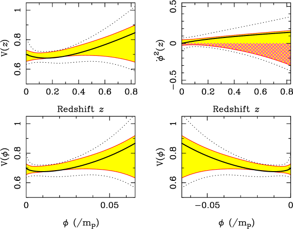
FIG. 3.: The effective potential $V(z)$, and the kinetic energy term ${\dot{\phi}}^{2}$, are shown in units of $\rho_{\rm cr}=3H_{0}^{2}/8\pi G$. Also plotted are the two forms of $V(\phi)$ for this $V(z)$, where the errors do not reflect errors in the $z$-$\phi$ relation. The value of $\phi$ (known up to an additive constant) is plotted in units of the Planck mass $m_{\rm P}$. The solid line corresponds to the best-fit values of the parameters. In each case, the shaded area covers the range of 68% errors, and the dotted lines the range of 90% errors. The hatched area represents the unphysical region ${\dot{\phi}}^{2}\!<\!0$.

Reconstructing the scalar field potential: We show the form of the effective potential $V(z)$ reconstructed using (5) in Fig. 3, along with the corresponding plot for $V(\phi)$, where $\phi$ is calculated by integrating (6). The field $\phi$ is determined up to an additive constant $\phi_{0}$, so we take $\phi$ to be zero at the present epoch ($z=0$).

Our experiments with several realizations of synthetic data show that this method works best if we fix the value of $\Omega_{\rm M}$. Henceforth, all reconstructed quantities are shown for $\Omega_{\rm M}=0.3$.

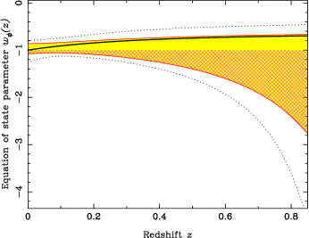
For a scalar field, the pressure $p\equiv-T^{\alpha}_{\alpha}={1\over 2}\dot{\phi}^{2}-V$ and the energy density $\varepsilon\equiv T^{0}_{0}={1\over 2}\dot{\phi}^{2}+V$ are related by the equation of state,

$$w_{\phi}(x)\equiv{p\over\varepsilon} = \frac{(2x/3)d\ln H/dx-1}{1-\left(H^{2}_{0}/H^{2}\right)\Omega_{\rm M}x^{3}}.$$ (12)

For the Cosmological constant, $w\!=\!-1$, while quintessence models [13] generally require $-1\!\leq\!w\!\leq\!0$ for $z\!\mathrel{\hbox to0.0pt{\lower 3.0pt\hbox{$\mathchar 536\relax$}\hss}\raise 2.0pt\hbox{$\mathchar 316\relax$}}\!2$.

Our reconstruction for $w_{\phi}(z)$ according to (12) is plotted in Fig. 4. There is some evidence of possible evolution in $w_{\phi}$ with $-1\!\leq\!w_{\phi}\!\mathrel{\hbox to0.0pt{\lower 3.0pt\hbox{$\mathchar 536\relax$}\hss}\raise 2.0pt\hbox{$\mathchar 316\relax$}}\!-0.86$ preferred at the present epoch, and $-1\!\leq\!w_{\phi}\!\mathrel{\hbox to0.0pt{\lower 3.0pt\hbox{$\mathchar 536\relax$}\hss}\raise 2.0pt\hbox{$\mathchar 316\relax$}}\!-0.66$ at $z=0.83$, the farthest SN in the sample (both at 68% confidence, upper limits correspond to $-0.80$ and $-0.46$ at 90% confidence respectively). However, a cosmological constant with $w=-1$ is consistent with the data.

FIG. 4.: The equation of state parameter $w_{\phi}(z)\!=\!P/\rho$ as a function of redshift. The solid line corresponds to the best-fit values of the parameters. The shaded area covers the range of 68% errors, and the dotted lines the range of 90% errors. The hatched area represents the region $w_{\phi}\!\leq\!-1$, which is disallowed for a minimally coupled scalar field.

The errors quoted in this paper are calculated using a Monte-Carlo method, where, in a region around the best-fit values of the parameters shown in Table 1, random points are chosen in parameter space from the probability distribution function given by the $\chi^{2}$-function that is minimized to yield the best fit. At each value of $z$ in the given range, the function in question is evaluated at over $10^{7}$ such points, and the errors enclosing 68% and 90% of all the values centered on the median are shown in the figures.

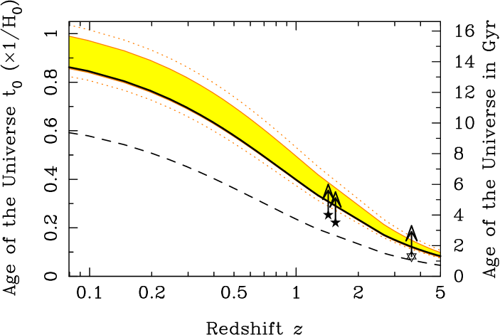
The ages of objects: Our ansatz (7) also provides us with a model-independent means of finding the age of the universe at a redshift $z$,

$$t(z)=H_{0}^{-1}\int_{z}^{\infty}\frac{dz^{\prime}}{(1+z^{\prime})h(z^{\prime})},$$ (13)

where the value of $h(z)\equiv H(z)/H_{0}$ is determined from (2). Figure 5 shows the age of the Universe at a given $z$ and compares it with the ages of two high redshift galaxies and the quasar B1422+231 [14]. We find that the requirement that the Universe be older than any of its constituents at a given redshift is consistent with our best-fit model, which is a positive feature since a flat matter-dominated Universe must have an uncomfortably small value of $H_{0}$ to achieve this.

FIG. 5.: The age of the Universe at a redshift $z$, given in units of $H_{0}^{-1}$ (left vertical axis) and in Gyr, for the value of $H_{0}\!=\!61.3$ km s^-1 Mpc^-1 (right vertical axis). The shaded region represents the range of 68% errors, and the dotted lines the range of 90% errors. The three high-redshift objects for which age-dating has been published [14] are plotted as lower limits to the age of the Universe at the corresponding redshifts. The dashed curve shows the same relation for an ($\Omega_{\rm M},\Omega_{\phi}$)=(1,0) Universe for the same $H_{0}$.

Discussion: In this letter, we have proposed a simple, analytical, three parameter ansatz describing the luminosity distance as a function of redshift in a flat FRW universe. The form of this ansatz is very flexible and can be applied to determine $D_{L}$ either from supernovae observations (as we have done) or from other cosmological tests such as lensing, the angular size-redshift relation etc. Using the resulting form of $D_{L}$ we reconstruct the potential of a minimally coupled scalar $\Lambda$-field (or quintessence) and its equation of state $w_{\phi}(z)$. It should be noted that the basic equations of this ansatz: (2), (7), (12) & (13) are flexible and can be applied to models other than those considered in the present paper. For instance one can venture beyond minimally coupled scalar fields by dropping either one or both of the constraints (9) & (10) (this is equivalent to removing the constraint $\rho_{\Lambda}+p_{\Lambda}\!\geq\!0$ on the $\Lambda$-field). Even with the limited high-$z$ data currently available, our ansatz gives interesting results both for the form of $V(\phi)$ as well as $w_{\phi}(z)$. As data improve, our reconstruction promises to recover ‘true’ model-independent values of $V(\phi)$ and $w_{\phi}(z)$ with unprecedented accuracy, thereby providing us with a deep insight into the nature of dark matter driving the acceleration of the universe.

Acknowledgments: TDS thanks the UGC for providing support for this work. VS acknowledges support from the ILTP program of cooperation between India and Russia. AS was partially supported by the Russian Foundation for Basic Research, grant 99-02-16224, and by the Russian Research Project “Cosmomicrophysics”.