A Model for Structure Formation Seeded by Gravitationally Produced Matter

Abstract

This model assumes the baryons, radiation, three families of massless neutrinos, and cold dark matter were mutually thermalized before the baryon number was fixed, primeval curvature fluctuations were subdominant, and homogeneity was broken by scale-invariant fluctuations in a new dark matter component that behaves like a relativistic ideal fluid. The fluid behavior could follow if this new component were a single scalar field that interacts only with gravity and with itself by a pure quartic potential. The initial energy distribution could follow if this component were gravitationally produced by inflation. The power spectra of the present distributions of mass and radiation in this model are not inconsistent with the measurements but are sufficiently different from the adiabatic cold dark matter model to allow a sharp test in the near future.

1. Introduction

One motivation for the search for alternative models for structure formation is that we arrived at the commonly discussed adiabatic cold dark matter (aCDM) picture after just a few false starts. This might be because the early universe is simple enough that there are only a few ways structure could have originated, or because we were lucky, or perhaps because more than one model is viable at the present level of constraints. It seems prudent to continue the search for viable alternatives before we learn whether they are needed.

The candidate presented here draws elements from a phenomenological model (Hu 1999) that allows an acceptable fit to the measured power spectra of distributions of matter and radiation, and a model with a physical provenance within the inflation scenario (Peebles 1999a) but a poorer fit to the measurements. Our new picture has the observational advantage of the former and a physical basis that simplifies the latter. It has elements in common with the phenomenological models analyzed by Bucher, Moodley, & Turok (1999), but crucial differences that make the present model viable.

We start with the idea that, since the dark matter may interact only weakly with ordinary matter and radiation, some or all of it may interact only with gravity (Peebles & Vilenkin 1999a; 1999b, hereafter PVb). Such dark matter would be gravitationally produced, as a squeezed state, by inflation (Ford 1987; Grishchuk & Sidorov 1990).

We discuss initial conditions from inflation in the next section, evolution of the departures from homogeneity in §3, and tests of the power spectra of the matter and radiation in §4.

2. Initial Conditions

The dynamical components are the cosmic microwave background (the CMB), three families of massless neutrinos, baryons, cold dark matter (CDM), and a new dark component that acts like an ideal fluid with the equation of state $p_{y}=\rho_{y}/3$. The primeval energy density contrasts satisfy

$$\delta_{\gamma}=\delta_{\nu}={4\over 3}\delta_{b}={4\over 3}\delta_{c}=-\delta_{y}\rho_{y}/(\rho-\rho_{y}).$$ (1)

The last part expresses the isocurvature condition, where $\rho$ is the total mass density in which the baryons and CDM are initially subdominant. The power spectrum of $\delta_{y}$ is nearly scale-invariant: $k^{3}P_{y}(k)$ is initially close to constant. The first part of equation (1) says the fluctuations in the usual matter components are adiabatic. This can follow if the chemical potentials of the neutrinos and CDM vanish and all these components are in mutual thermal equilibrium that is broken after the baryon number is frozen and before the CDM is nonrelativistic. The relativistic fluid behavior of $\rho_{y}$ can follow from a field that interacts only with gravity and with itself by a quartic potential, with the action

$$S=\int a^{3}d^{3}x\,dt\,(y_{,i}y^{,i}/2-\lambda y^{4}/4),$$ (2)

and energy density $\rho_{y}=\dot{y}^{2}/2+(\nabla y)^{2}/2+\lambda y^{4}/4$.

When the frequency of the field oscillation is large compared to the Hubble parameter $\dot{a}/a$, equation (2) expressed in conformal time $\tilde{t}=\int dt/a(t)$ is the action in Minkowski coordinates for $\tilde{y}=ay$. Since the energy of $\tilde{y}$ in Minkowski spacetime is conserved, the mean energy density in $y$ scales as $\rho_{y}\propto a(t)^{-4}$ (Ford 1987, Peebles 1999b). This means $\rho_{y}$ can be large enough to serve as a primeval seed for structure formation but remain small enough not to interfere with the standard models for light element production and gravitational structure formation.

Fluctuations in $\rho_{y}$ are well approximated as linear acoustic waves from the end of inflation, when the field starts oscillating, through the characteristic acoustic oscillation time divided by the density contrast (Peebles 1999b). The acoustic wave model fails with the appearance of features that resemble shock waves. If the scale-invariant spectrum of $y$ extends to small wavelengths these shock-like features appear well before the field fluctuations of interest to astronomy appear at the Hubble length. The analysis in Peebles (1999b) indicates that this does not spoil the acoustic wave model on larger scales.

If the field $y$ in equation (2) exists it will have been excited, with a near scale-invariant spectrum, by inflation (Ford 1987). Kofman & Linde (1987) considered the near classical evolution of $y$ in inflation when the potential for the inflaton $\phi$ also is quartic, $V(\phi)=\lambda_{\phi}\phi^{4}/4$. We assume this same eternal inflation model.

We assume the dimensionless parameter in equation (2) is in the range

$$\lambda_{\phi}\ll\lambda<0.01.$$ (3)

The lower bound makes the $y$-field energy subdominant to the inflaton during inflation (PVb); otherwise $y$ assumes the role of the inflaton (Felder, Kofman & Linde 1999). The upper bound is chosen so $y$ is close to constant across the present Hubble length. This follows from a consideration of the competition between the freezing of quantum fluctuations that tend to drive the field value away from zero and classical dissipation as the field rolls to the minimum of its potential at $y=0$. Early in inflation these processes are close to statistical equilibrium. As the value of the Hubble parameter $H$ decreases equilibrium eventually is broken, at expansion parameter $a_{e}$, and $y$ thereafter evolves almost as a classical field. Under the upper bound in equation (3) the expansion from $a_{e}$ to the end of inflation is large enough that $y$ is close to constant across our Hubble length. We assume that at our position the field value at $a=a_{e}$ is close to the characteristic value at equilibrium, $\lambda\left<y^{4}\right>=3H^{4}/8\pi^{2}$ (Starobinsky & Yokoyama 1994). The perturbations to $y$ added from $a=a_{e}$ to the end of inflation produce a near Gaussian scale-invariant fluctuation spectrum with variance per logarithmic interval of wavenumber (PVb eq. [39])

$$\left(\delta y\over y\right)^{2}\approx{\lambda\over 6\pi^{2}\log_{e}a_{x}/a_{p}}.$$ (4)

As discussed in the next section the large-scale perturbation to the present thermal background radiation (the CMB) is $\delta T/T=(\delta y/y)/5f$, where $f$ is the ratio of mass densities in radiation and neutrinos to the energy in the $y$-field. The fit to the observed temperature variance per logarithmic interval of $l$, $(\delta T/T)^{2}=(1\times 10^{-5})^{2}$, requires

$$\lambda\approx 1\times 10^{-5}f^{2}.$$ (5)

The value of $f$ depends on the model for the origin of ordinary matter and radiation; we must treat $f$ as an adjustable parameter. The standard model for the light elements requires $f\gtrsim 10$, leaving a small window of consistency between equations (3) and (5).

3. Evolution

The evolution of the distributions of matter and radiation in linear perturbation theory is computed by the usual methods. We discuss only aspects that differ from the usual case.

The dynamics of the fluctuations are governed by two events: the transition from radiation- to matter-dominated expansion, and Hubble crossing, when relativistic stress gradients and gravity have comparable dynamical effects. We consider first a large-scale mode that crosses the Hubble length after matter-radiation equality. The residual entropy fluctuation,

$$\sigma=\delta_{c}-{3\over 4}\delta_{\rm rel}\approx\delta_{c}={3\over 4}\delta_{\gamma}\,$$ (6)

where $\rho_{\rm rel}=\rho_{\gamma}+\rho_{\nu}+\rho_{y}$, becomes important near matter-radiation equality and before pressure causes the mode to oscillate. On these large scales the relative distribution of the $y$-field and the familiar radiation species is irrelevant because their gravitational effects exactly cancel before Hubble crossing and are negligible afterward. The relation between the present distributions of the cold dark matter and the CMB shows an interesting effect. The gravitational potential in the matter-dominated regime is related to the initial entropy fluctuation as $\Phi={\sigma/5}$, and $\Phi$ is related to the density perturbation by the Poisson equation (Kodama & Sasaki 1986). The CMB anisotropy due to the gravitational redshift is

$${\delta T\over T}\Big{|}_{\rm grav}=-2\Delta\Phi+{\delta T\over T}\Big{|}_{\rm init}=-{1\over 3}\Phi\,.$$ (7)

This is the same as the adiabatic CDM (aCDM) model, and different from the isocurvature CDM (iCDM) model in Peebles (1999a) where primeval fluctuations in the CDM are balanced by the CMB and neutrinos and $\delta T/T|_{\rm grav}=-2\Phi$. It is helpful to the construction of a viable model to assume the initial photon distribution follows that of the species that is responsible for gravitational structure formation in the matter-dominated epoch (Hu 1999). This puts the photons that initially are hottest where the gravitational potential becomes the deepest, so the temperature fluctuation is reduced as the photons move out of the potential well. The consequence is that in aCDM and the present model the observed ratio of matter to radiation fluctuations follows from a near scale-invariant primeval fluctuation spectrum, while in the iCDM model a fit to this ratio requires a substantial tilt to increase small-scale fluctuations over large.

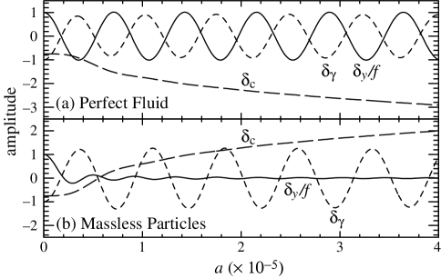
Figure 1.— Time evolution of Fourier amplitudes in a mode with very short comoving wavelength for (a) our perfect fluid model for the $y$-component and (b) a free massless particle model. Note the zero crossing of the CDM amplitude $\delta_{c}$ in (b). In a mode at $k\sim 0.15h$ Mpc^-1, $\delta_{c}$ crosses zero near matter-radiation equality, producing the zero of $P(k)$ in the dashed line in Fig. 2.

The evolution of small-scale fluctuations in the CDM that cross the Hubble length before matter-radiation equality is surprisingly sensitive to the behavior of the new $y$-component. At Hubble crossing, stress gradients in the relativistic components cause them to oscillate. The CMB density oscillates as an acoustic (sound) wave with amplitude given by the initial conditions in such a way that observationally acceptable peaks result from scale-invariant initial conditions. The $y$-component in our model also oscillates as an acoustic wave. Aside from the neutrinos, this keeps the radiation distributions almost balanced. The CDM amplitude appears at the Hubble length after moderate growth from the initial value (Fig. 1a). As in aCDM, the modest further increase of $\delta_{c}$ to matter-radiation equality leaves the usual $k^{-2}$ suppression of small-scale power and an observationally acceptable present mass fluctuation spectrum from initially scale-invariant fluctuations. If instead the $y$-component were a free gas of massless particles, free streaming would cause an imbalance with the acoustic oscillation of the CMB, as in Figure 1b. The resulting metric perturbation reverses the sign of $\delta_{c}$. The reversal can only be produced during the radiation-dominated epoch, so there is a mode near the Hubble scale at matter-radiation equality that is caught in the act of reversal, producing a zero in the linear power spectrum, and spoiling the fit to large-scale structure measurements.

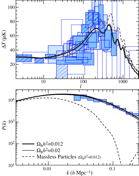
Figure 2.— Measured and modeled power spectra of the CMB and galaxy distributions. The shading of the CMB error boxes is according to area and corresponds to the $1\sigma$ errors $\times$ the width of the experimental window; cross hatching denotes measurements included in set “A”. Our models are plotted as solid curves; the dashed curve represents a model where the seed field is a gas of free massless particles rather than a fluid.

4. Phenomenology

Figure 2 compares our model predictions to all significant measurements of the CMB temperature anisotropy and to the Peacock & Dodds (1994) compilation of measurements of the power spectrum of the galaxy distribution. We assume a scale-invariant initial spectrum of fluctuations in $y$ (as in eq. [4]), standard recombination, $\Omega_{m}=0.35$, $\Omega_{\Lambda}=0.65$, $h=0.8$, and two values of the baryon density, $\Omega_{b}h^{2}=0.02$ and $\Omega_{b}h^{2}=0.012$. The former is close to the central value of Burles et al. (1999) based on the deuterium abundance ${\rm D/H}=3.4\times 10^{-5}$. Kirkman et al. (1999) consider the most secure bound to be ${\rm D/H}<6.7\times 10^{-5}$; this abundance scales the baryon density to the lower number.

Following Tegmark (1999) and Miller et al. (1999), we find a crude estimate of $\chi^{2}$ for the CMB temperature anisotropy by treating all data points as independent with Gaussian distributions of errors. The first two lines of Table 1 list the reduced $\chi^{2}$ employing all the data (58 points), the selection in Miller et al. (1999) (“A”; 24 points), and the remaining data plus the COBE DMR results (“B”; 42 points). The third line is the best fit aCDM model from Tegmark (1999). Values for the full data set and selection “B” are arguably less secure because they are based on a more heterogeneous set of methods. The $\sim 10\%$ calibration uncertainty, which is not included in these $\chi^{2}$ estimates, is a serious general barrier to the interpretation in terms of formal measures of significance. Within the calibration uncertainty our low baryon density model seems viable, although challenged by the D/H measurements (Kirkman et al. 1999), while our high density model is challenged but we believe not ruled out by the CMB measurements.

TABLE 1

Approximate CMB $\chi^{2}/\nu$

Model	All	A	B
$\Omega_{b}h^{2}=0.012$	2.6	1.5	1.3
$\Omega_{b}h^{2}=0.02$	2.7	2.0	1.3
aCDM	2.5	1.2	1.4

We get satisfactory agreement with the power spectrum of the galaxy distribution. The normalization implies $\sigma_{8}=0.84-0.86$, consistent with the bounds $0.74\lesssim\sigma_{8}\lesssim 1.1$ implied by the abundance of rich clusters of galaxies at our model parameters (e.g. Viana & Liddle 1999).

Our model differs from those of Bucher et al. (1999) in two ways. First, the CDM density perturbations follow the CMB (eq. [1]). We noted that this suppresses the large-scale anisotropy of the CMB, allowing a near scale-invariant primeval spectrum and making the peaks in the anisotropy spectrum at $\ell>100$ more prominent. The same effect follows from a coherent superposition of the CDM-isocurvature and neutrino isocurvature modes of Bucher et al. (1999); one cannot use a linear combination of the individual power spectra. Second, motivated by equation (2), we model the isocurvature departure from homogeneity by a component that behaves as a perfect fluid rather than a gas of free massless particles. One sees in Figure 1 and the dashed curves in Figure 2 that the CMB anisotropy is not much affected but the free particle model produces a zero in the mass power spectrum (in linear perturbation theory) at an undesirable wavelength.

The power spectra of the present distributions of matter and the CMB depend on the cosmological parameters in different ways from the aCDM model. The heights of the peaks in the CMB spectrum depend on $\Omega_{b}h^{2}$ in opposite ways (Hu & White 1996): here the odd-numbered peaks represent rarefaction of the photon fluid in the potential wells and hence decrease when the baryon density is increased, as one sees in Figure 2. Also, since our model has no initial metric fluctuations whose decay in the radiation-dominated epoch enhance the peaks, the peak values do not increase with decreasing $\Omega_{m}h^{2}$. The lesson here is a general one: cosmological parameters derived from a model fit are provisional no matter how securely fixed within the model until the model is unambiguously established.

5. Discussion

We conclude that our model is viable but likely to be critically tested by CMB anisotropy measurements in progress. The same is true of the aCDM model, of course.

Our model can be adjusted; here are four considerations. First, we use isocurvature initial conditions. There may be a significant adiabatic perturbation from the inflaton, or, in other inflation models, from the stress of the $y$-field fluctuations during inflation. Second, we place $\lambda$ in a narrow window (eqs. [3] and [5]). If $\lambda\gtrsim 0.01$ the fluctuations in $\rho_{y}$ at the end of inflation have positive skewness, so the primeval fluctuations in the CDM mass distribution are non-Gaussian with negative skewness. Models with positive skewness are seriously constrained (Frieman & Gaztañaga 1999); negative skewness may be interesting for structure formation. The second moments needed for the tests in Section 4 have not been analyzed for this case. Third, one may ask whether some or all of the CDM is in fields that interact only with gravity and themselves by potentials that would have to be more complicated than the quartic considered here. PVb present preliminary elements of a model for this more complicated case. Fourth, we have assumed standard recombination. One could imagine stars present at $z\sim 1000$ delay the rapid drop in ionization; that would shift the peaks in the CMB spectra to smaller $\ell$ and substantially change the significance of this test.

The field $y$ is a new hypothesis. Its parameter $\lambda$ is not exceedingly small, however, and by moving the seed for structure formation from the inflaton we remove the requirement for a specific value of the very small parameter $\lambda_{\phi}$. But closer consideration of these issues might best await observational developments.

It may be significant that the structure formation history in our model is only mildly different from aCDM. Perhaps this is telling us viable phenomenological models already are limited: they have to approximate aCDM. Or perhaps our imagination in exploring concepts like gravitationally produced matter is limited.

References

- (1) Bucher, M., Moodley, K. & Turok, N. 1999, astro-ph/9904231
- (2) Burles, S., Nollett, K.M., Truran, J.N., & Turner, M.S., 1999 PRL, 82, 4176
- (3) Felder, G., Kofman, L. & Linde, A. D. 1999 hep-ph/9903350
- (4) Ford, L. H. 1987, Phys Rev, D35, 2955
- (5) Frieman, J. & Gaztañaga. E. 1999, astro-ph/9903423
- (6) Grishchuk, L.P. & Sidorov, Y. V. 1990, Phys Rev D, 42, 3413
- (7) Hu, W. 1999, Phys Rev, D59, 021301
- (8) Hu, W. & White, M. 1996, ApJ, 471 30
- (9) Kirkman, D., Tytler, D., Burles, S., Lubin, D., and O’Meara, J. M. 1999, astro-ph/9907128
- (10) Kodama, H. & Sasaki, M. 1986, Int. J. Mod. Phys., A1, 265
- (11) Kofman, L. & Linde, A. D. 1987, Nucl Phys, B282, 555
- (12) Miller, A. D. et al. 1999, ApJ, 524, L1
- (13) Peacock, J.A. & Dodds, S.J. 1994, MNRAS, 267 1020
- (14) Peebles, P. J. E. 1999a, ApJ, 510, 531
- (15) Peebles, P. J. E. 1999b, preprint
- (16) Peebles, P. J. E. & Vilenkin, A. 1999a, Phys Rev, D59, 063505
- (17) Peebles, P. J. E. & Vilenkin, A. 1999b, Phys Rev, in press; PVb
- (18) Starobinsky, A. A. & Yokoyama, J. 1994, Phys Rev D50, 6357
- (19) Tegmark, M. 1999, ApJL, 514, 69
- (20) Viana, P.T.P & Liddle, A. 1999, MNRAS, 303, 535