Jet driven molecular outflows in Orion

Abstract

We present high sensitivity and high angular resolution images of the high velocity ($v_{LSR}>30\,$km s^-1) CO emission in the $J=1\rightarrow 0$ and $J=2\rightarrow 1$ lines of the OrionKL region. These results reveal the morphology of the high-velocity CO emission at the most extreme velocities. High velocity emission have been only detected in two regions: BN/KL (IRc2/I) and Orion–S.

The Orion–S region contains a very young (dynamical age of $\sim 10^{3}\,$years), very fast ($\sim 110\,$km s^-1) and very compact ($\buildrel<\over{\sim}$$0.16\,$pc) bipolar outflow. From the morphology of the high-velocity gas we estimate that the position of the powering source must be $20^{\prime\prime}$ north of FIR$\,4$. So far, the exciting source of this outflow has not been detected. For the IRc2/I molecular outflow the morphology of the moderate velocity ($\buildrel<\over{\sim}$60 km s^-1) gas shows a weak bipolarity around IRc2/I. The gas at the most extreme velocities does not show any bipolarity around IRc2/I, if any, it is found $\sim 30^{\prime\prime}$ north from these sources. The blue and redshifted gas at moderate velocities shows similar spatial distribution with a systematic trend for the size of the high-velocity gas to decrease as the terminal radial velocity increases. The same trend is also found for the jet driven molecular outflows L 1448 and IRAS$\,03282+3035$. The size-velocity relationship is fitted with a simple velocity law which considers a highly collimated jet and entrained material outside the jet moving in the radial direction. We also find that most of the CO outflowing at moderate velocities is located at the head of the jet. Our results and the spatial distribution and kinematics of the shock tracers in this outflow can be explained if the IRc2/I outflow is driven by a precessing jet oriented along the line of sight. The implication of these findings in the evolution of molecular outflows is discussed.

Key words: ISM: clouds – ISM: jets and outflows – nebulae: Orion Nebula – Stars: formation – Stars: mass-loss – shock waves

1 Introduction

The Orion Molecular Cloud (hereafter OMC 1) has played a central role in the study of the formation and evolution of high$-$mass stars. This molecular cloud harbors massive stars in the stage of energetic mass loss. Two regions contain high-velocity (HV hereafter) molecular outflows, the IRc2/I outflow in the BN/KL nebula and the Orion–S region.

The first evidence of massive star formation in the Orion–S region, located $\sim 100^{\prime\prime}$ south of IRc2 came from the presence of warm gas (Ziurys et al., 1981) and large dust column densities (Keene, Hildebrand & Whitcomb, 1982). Subsequent observations of CO with higher angular resolution showed the presence of a long filament at moderate velocities ($\leq 30\,$km s^-1) which has been interpreted as a redshifted monopolar jet powered by FIR 4 (Schmid$-$Burgk et al., 1990). H₂O masers have been detected in the vicinity of FIR 4 but they are not related with the monopolar jet (Gaume et al., 1998). In fact, the H₂O masers seem to be associated with the very fast bullets ($\mid v_{LSR}\mid>50\,$km s^-1) found in the compact bipolar outflow recently detected by Rodríguez–Franco et al. (1999) which is perpendicular to the low velocity jet.

Due to its nearness and intense CO emission, the prominent high-velocity CO outflow in the KL nebula has been the subject of intense study in several rotational transitions of this molecule (Kwan & Scoville, 1976; Zuckerman, Kuiper & Rodríguez$-$Kuiper, 1976; Wannier & Phillips, 1977; Phillips et al., 1977; Goldsmith et al., 1981; Van Vliet et al., 1981). The first observations showed the presence of outflowing gas at velocities up to $100\,$km s^-1 from the cloud velocity. Strong shocks produced by the interaction of the outflow from the powering source with the ambient material gives rise to strong emission of vibrationally excited molecular hydrogen H${}_{2}^{*}$ (see e.g. Nadeau & Geballe, 1979), H₂O masers around the source IRc2/I (Gaume et al, 1998) and molecules like SiO, SO, SO₂ (Wright et al., 1996) produced by shock chemistry.

In spite of the large numbers of observations of this molecular outflow, its nature is so far unclear. Observations with high angular resolution of the HV CO emission at moderate velocities (Erickson et al., 1982; Chernin & Wright, 1996) have shown a weak bipolarity of the outflow. Based on these observations, it was proposed that this outflow is a conical outflow with a wide ($130^{\rm o}$) opening angle, oriented in the southwest$\leftrightarrow$northeast direction. This is powered by source I (Chernin & Wright, 1996). However the wide opening angle model cannot account for a number of observational facts such as the spatial distribution and kinematics of the high and low velocity H₂O and the SiO masers (Greenhill et al., 1998; Doeleman et al., 1999). Furthermore, the morphology of the HV CO emission at intermediate velocities shows that the outflow is offset from IRc2/I by $10^{\prime\prime}$ indicating that a complex channeling of the HV gas is needed if IRc2/I is the powering source (Wilson et al., 1986). Recently Rodríguez–Franco et al. (1999) has mapped the IRc2/I molecular outflow with high sensitivity. The spatial distribution of the most extreme velocity shows the lack of bipolarity around IRc2/I as expected from the wide opening angle model. These maps also reveal a ring-like structure of high-velocity bullets which also are difficult to account for if the outflow has a wide opening angle. Rodríguez–Franco et al. (1999) have proposed that the ring of the HV CO bullets and the distribution and kinematics of the H₂O masers could be explained if the outflow is driven by a precessing jet oriented along the line of sight. If this is the explanation, this will allow us to specify the main entrainment mechanism in molecular outflows (see e.g. Raga & Biro, 1993; Cabrit, 1995).

In this paper we present new maps of the CO emission and analyze in detail the morphology of the CO emission at moderate and extreme velocities in the IRc2/I and Orion–S molecular outflows, and present new arguments supporting the idea that the Orion outflows are young and driven by high velocity jets.

2 Observations and results

The observations of the $J=2\rightarrow 1$ and the $J=1\rightarrow 0$ lines of CO where carried out with the IRAM 30$-$m telescope at Pico Veleta (Spain). Both rotational transitions were observed simultaneously with SIS receivers tuned to single side band (SSB) with an image rejection of $\sim 8\,$dB. The SSB noise temperatures of the receivers at the rest frequencies for the CO lines were 300 K and 110 K for the $J=2\rightarrow 1$ and the $J=1\rightarrow 0$ lines, respectively. The half power beam width (HPBW) of the telescope was $12^{\prime\prime}$ for the $J=2\rightarrow 1$ line and $24^{\prime\prime}$ for the $J=1\rightarrow 0$ line. As spectrometers, we used two filter banks of $512\times 1\,$MHz that provided a velocity resolution of 1.3 and 2.6 km s^-1 for the $J=2\rightarrow 1$ and the $J=1\rightarrow 0$ lines of CO, respectively. The observation procedure was position switching with the reference taken at a fixed position located 15^′ away in right ascension. The mapping was carried out by combining 5 on$-$source spectra with one reference spectrum. The typical integration times were 20 sec for the on-positions and 45 sec for the reference spectrum. The rms sensitivity of a single $J=2\rightarrow 1$ spectrum is 0.6 K. Pointing was checked frequently on nearby continuum sources (mainly Jupiter) and the pointing errors were $\buildrel<\over{\sim}$4^′′. The calibration was made by measuring sky, hot and cold loads. The line intensity scale is in units of main beam brightness temperature, using main beam efficiencies of 0.60 for the $J=1\rightarrow 0$ line and 0.45 for the $J=2\rightarrow 1$ line.

We have made an unbiased search for high-velocity molecular gas in OMC 1 by mapping with high sensitivity the $J=1\rightarrow 0$ and $J=2\rightarrow 1$ lines of CO in a region of $14^{\prime}\times 14^{\prime}$ around IRc2/I. In this article we will analyze the very high-velocity gas associated to molecular outflows. The widespread CO emission with moderate velocities ($\mid v_{LSR}-9\mid$$\buildrel<\over{\sim}$40 km s^-1) will be discussed elsewhere (Martín$-$Pintado & Rodríguez$-$Franco, 2000). In our CO maps we have only detected the known molecular outflows with $\mid v_{LSR}-9\mid$$\buildrel>\over{\sim}$30 km s^-1, IRc2 and Orion$-$S. Figure 1 shows a sample of line profiles taken towards selected positions around IRc2 and Orion$-$S.

3 High-velocity gas around IRc2/I

3.1 The morphology

Fig. 2 shows the spatial distribution of the CO $J=2\rightarrow 1$ integrated intensity emission around IRc2 for radial velocity intervals of 20 km s^-1 for the blueshifted and redshifted gas. The spatial distribution of the HV gas with moderate velocities ($\buildrel<\over{\sim}$60 km s^-1), hereafter MHV, in our data is similar to that observed by Wilson et al. (1986). Our new maps have better sensitivity. These reveal for the first time the spatial distribution of the high-velocity gas for the most extreme velocities ($\mid v_{LSR}\mid>60\,$km s^-1), hereafter EHV, of the molecular outflow which shows a different morphology from that of the MHV gas.

The maximum of the CO emission for the blueshifted gas always appears northwest of IRc2/I. The offset between the CO maximum and IRc2 systematically increases from 10^′′ for radial velocities of $-$40 km s^-1 up to 25^′′ for the gas at $-$110 km s^-1. The location of the redshifted CO emission maxima does not show such a clear trend. At moderate velocities (up to 75 km s^-1), the maximum CO emission occurs in a ridge with two peaks of nearly equal intensity located southeast and northwest of IRc2/I. The northwest peak of the redshifted emission occurs at the same position as the blueshifted peak for lower radial velocities. For the most redshifted gas ($\sim$100 km s^-1), the CO emission breaks up into several condensations located around IRc2/I. For this radial velocity, the most intense CO condensation peaks as for the blueshifted gas, northwest of IRc2, there is weaker emission found 20^′′ west and southeast of IRc2/I.

Fig. 3a and b summarize the distribution of the high-velocity molecular gas in Orion for moderate and extreme velocities. The new data show that the MHV molecular gas around IRc2 (fig. 3a) has a very different morphology than that of the EHV gas (fig. 3b). At moderate velocities, the CO emission shows a very weak bipolarity (if any) around IRc2 in the southeast$\leftrightarrow$northwest direction (see Fig. 3a). For radial velocities close to the terminal velocity, the strongest CO emission (see Fig. 3b) does not show any bipolarity around IRc2/I. The only possible bipolar morphology is observed around a position located $\sim$20^′′ northwest of IRc2 and $10^{\prime\prime}$ south of IRc9 represented as a filled square in Fig. 3.

3.2 The size-velocity relation in the HV gas

The terminal velocities of the blue and redshifted MHV gas show similar spatial distribution with an elliptical–like shape centred in the vicinity of IRc2/I, and a systematic trend of the size of HV gas to decrease as a function of the velocity (see Fig. 2). These two characteristics are illustrated in Fig. 3c and d where we plot the dependence of the size of the HV CO emission as a function of the terminal velocity for the red and the blue shifted gas respectively. The contours in these figures shows the location of the gas with the same terminal velocity. The area enclosed by a given contour level corresponds to the region which contains HV molecular gas with terminal velocities larger than that of the contour level. For moderate velocities ($\buildrel<\over{\sim}$60 km s^-1), the size of HV gas is $\sim$110^′′ and decreases to $\sim$40^′′ for the extreme velocities. The HV gas, for most radial velocities, is concentrated in a region with an elliptical like shape centered at ($-4^{\prime\prime}$, $4^{\prime\prime}$) with respect to IRc2/I.

3.3 High-velocity “Bullets”

The detection of these high velocity bullets in the Orion IRc2/I outflow has been reported by Rodríguez–Franco et al. (1999). For completeness, we summarize the main characteristics. Fig. 1 shows several examples of CO profiles towards the IRc2/I region where the location of the HV bullets are shown by vertical arrows. The typical line-width of the CO HV bullets is $20-30\,$km s^-1, these are distributed in a ring like structure of size $\sim 10^{\prime\prime}\times 50^{\prime\prime}$ ($0.02\times 0.1\,$pc) and thickness $12^{\prime\prime}-20^{\prime\prime}$ ($0.02-0.04\,$pc) with IRc2 located in the southeast edge of the HV bullets rings (see fig. 3e and f).

4 High velocity gas around Orion–S

4.1 The morphology and characteristics of the high-velocity bipolar outflow Orion–S

Moderate high velocity gas ($\leq 30\,$km s^-1) have been detected in this region in CO and SiO (Schmid–Burgk et al. 1990; Ziurys & Friberg, 1987). The CO emission with moderate velocities has been associated to a monopolar outflow (low velocity redshifted jet) in Orion–S discovered by Schmid–Burgk et al. (1990). Rodríguez–Franco et al. (1999) reported the detection of a new compact and Fast Bipolar Outflow (hereafter Orion-South Fast Bipolar Outflow, or Orion-SFBO) with terminal velocities of $\sim 100\,$km s^-1. In this work, we will present the main features of this new outflow. To avoid the confusion with other HV features in Orion–S, such as H II region (see Martín–Pintado et al., 2000) and the monopolar outflow (Schmid–Burgk et al. 1990) we will consider only the CO emission for radial velocities in the range $<-5\,$km s^-1, and $>25\,$km s^-1. Fig. 4a shows the integrated intensity map in the $J=2\rightarrow 1$ rotational transition of CO for the blueshifted (solid contours) and the redshifted line wings (dashed contours) of the Orion$-$SFBO. This new outflow shows a clear bipolar structure in the southeast$\leftrightarrow$northwest direction, just perpendicular to the low velocity redshifted jet.

The morphology of the Orion$-$SFBO suggests that the axis of the bipolar outflow is oriented close to the plane of the sky. The blueshifted emission peaks $40^{\prime\prime}$ northwest of FIR 4 while redshifted gas has its maximum intensity $15^{\prime\prime}$ northeast from that source. Since the morphology of the bipolar SiO emission (Ziurys & Friberg, 1987) is similar to the CO emission reported in this paper, the SiO emission is very likely related to the Orion$-$SFBO rather than to the low velocity monopolar jet (Schmid–Burgk et al., 1990).

The structure of the HV gas in the Orion$-$SFBO as a function of the radial velocities is shown in Fig. 4b. The HV gas in the blue and redshifted wings have a different behavior. While the redshifted CO emission peak is located at the same spatial location for all radial velocities, the blueshifted CO peak moves to larger distance ($\sim 10^{\prime\prime}$, nearly one beam) from FIR 4 as the radial velocity increases from $-70$ to $-100\,$km s^-1. The most extreme velocities in the blue lobe (between $-80$ and $-110\,$km s^-1) arise from a condensation of $\sim 11^{\prime\prime}$ located $36^{\prime\prime}$ northwest from FIR 4. High velocity bullets (see vertical arrows in fig. 1) also appear in both the blue and the redshifted, lobes. A description can be found in Rodríguez–Franco et al. (1999).

	$v_{mt}$	Mass	Momentum	Energy
	(km s-1)	($M_{\odot}$)	($M_{\odot}$ km s-1)	(erg)
Wings
blue	$-140$	0.019	14.3	7.97$\times 10^{45}$
red	88	0.017	13.3	5.46$\times 10^{45}$
Bullets
blue	$-140$	3.4$\times 10^{-3}$	0.5	6.9$\times 10^{44}$
red	88	8.6$\times 10^{-3}$	0.7	5.6$\times 10^{44}$
1Maximum velocity
2For a CO abundance of $10^{-4}$
and excitation temperature of 80 K.

Table 1.: Physical parameter of the molecular outflow Orion–SFBO and the associated bullets.

4.2 Exciting source

The source(s) powering the high-velocity gas in Orion–S is, so far, unknown. The source FIR 4 has been proposed to be the exciting source of the low velocity jet (Schmid$-$Burgk et al., 1990). However, FIR 4 cannot be the powering source for this outflow, because this source is located $20^{\prime\prime}$ south from the geometrical center defined by the two lobes (see figure 4a). One can use the kinematics and the morphology of the HV gas to estimate the position of the exciting source. This procedure has been successfully used for outflows associated with low mass stars (see Bachiller et al., 1990). From the velocity$-$position diagram along the direction of the outflow axis we have estimated the location of the possible exciting source by considering that the source should be located at the position where the radial velocity changes from blue to redshifted. The inferred position of the exciting source using this procedure is located $20^{\prime\prime}$ north of FIR 4, and it is shown in Fig. 4 as a filled square.

In contrast to the outflows powered by low mass star where the exciting source appears as strong millimeter emitters and faint centimeter emitters, the source(s) of the Orion$-$SFBO has not been detected so far in the mm or cm continuum emission (see e.g. Gaume et al., 1998). The limit of the cm radio continuum emission is a factor of 10 smaller than the predicted by the relationship of Anglada et al. (1998) for collisional ionization. This could be due to an underestimation of the dynamical age of the outflow or more likely to a time variable jet (see section 6.3).

5 The physical conditions of the HV gas in the IRc2/I outflow and in Orion$-$SFBO

The H₂ densities of the HV gas in the IRc2/I outflow are high enough ($\sim 10^{5}\,$cm^-3, see Boreiko et al., 1989; Boreiko & Betz, 1989; Graf et al., 1990) to thermalize the low rotational ($J$) lines at a kinetic temperature of $\buildrel>\over{\sim}$$70\,$K (Boreiko et al., 1989). Under these conditions, one can estimate the opacities of the HV gas from the intensity ratio between the $J=2\rightarrow 1$ and the $J=1\rightarrow 0$ lines. Fig. 6 shows the profiles of the $J=2\rightarrow 1$ and the $J=1\rightarrow 0$ lines of CO and the ratio between the lines towards IRc2/I. In order to account for the different beam size in both lines, the $J=2\rightarrow 1$ line has been smoothed to the resolution of the $J=1\rightarrow 0$ line.

The expected contamination to the $J=1\rightarrow 0$ of CO by the recombination line H38$\alpha$ is also shown, as a dotted line, in the central panel of Fig. 6. Since the contribution of the recombination lines is negligible for the CO HV gas, we can use the CO line ratio over the whole velocity range. We are interested only in the relatively compact ($\buildrel<\over{\sim}$40^′′) emission of the HV gas in the IRc2/I region and therefore, the line intensity ratio in Fig. 6 have been calculated using the main beam brightness temperature scale. To obtain the corresponding ratio for extended sources, the values in fig. 6 should be divided by a factor 1.5; i.e. the ratio between the main beam efficiencies of the telescope for both lines.

The line ratio shows a remarkably symmetric distribution around 5 km s^-1 (the ambient cloud velocity) suggesting that possible contamination of the data from other molecular species emission must be negligible. For the ambient velocities of the gas (between 0 and 15 km s^-1) the emission is extended and the ratio of $\sim 1.5$ (1 in the $T_{a}^{*}$ scale) corresponds to the expected value for extended optically thick emission. As the radial velocity increases, the ratio increases up to values around 2.7 for velocities of $\mid v_{0}-v_{\rm LSR}\mid\sim 50\,$km s^-1. For this velocity range our results are consistent with those of Snell et al. (1984), once the contribution from the extended emission within their larger beam is take into account. For radial velocities larger than $\mid v_{0}-v_{\rm LSR}\mid\sim 50\,$km s^-1, the line ratio decreases again. The minimum value of 1.5 is close to the values expected for optically thick emission. This is present at $\pm 55\,$km s^-1, just at the radial velocity where the bullet features are found (Rodríguez–Franco et al., 1999). The smaller line ratio is consistent with the increase in the CO column density due to the CO HV bullets. The line ratio rises to its maximum value, 3.5, for radial velocities near to $\pm 70\,$km s^-1. These data suggest that CO emission for most of the velocity range is optically thin, except for the radial velocities where the bullets are found. Then, except for the CO HV bullets the CO integrated intensity can be translated directly into CO column of densities. Table 2 gives the physical characteristics for the outflow and the CO HV bullets. The opacity of the bullets is unknown. To derive the properties, we have assumed optically thin emission and the ring morphology observed by Rodríguez–Franco et al. (1999). This gives a lower limit to the mass in the CO bullet ring. The total mass in the bullet ring represents the $\stackrel{{\scriptstyle\scriptstyle>}}{{\scriptstyle\sim}}$20% of the total mass of the outflow.

	$v_{mt}$	Mass	Momentum	Energy
	(km s-1)	($M_{\odot}$)	($M_{\odot}$ km s-1)	(erg)
Wings
blue	$-121$	1.10	2.3$\times 10^{3}$	9.86$\times 10^{47}$
red	142	0.96	2.5$\times 10^{3}$	9.88$\times 10^{47}$
Bullets
blue	-100	0.23	23	2.30$\times 10^{46}$
red	80	0.43	34	2.88$\times 10^{46}$
1 Maximum terminal velocity
2It have been assumed a typical CO abundance of $10^{-4}$
and an excitation temperature of 80 K.

Table 2.: Physical parameter of the Orion KL molecular outflow and the associated bullets.

We have also estimated the physical parameters of the high velocity gas and of the bullets associated to the Orion$-$SFBO. We have assumed optically thin emission, LTE excitation at a temperature of 80 K, and a typical CO abundance of 10^-4. The results given in Table 1 show the characteristics for the molecular outflow and for the bullets. The characteristics of these CO HV bullets are similar to those found in low mass stars.

6 A jet driven molecular outflow in the IRc2/I region

The morphology, the presence of HV bullets, and the high degree of collimation of the Orion$-$SFBO are clear evidence that this outflow is jet driven, with the jet oriented close to the plane of the sky (see also Rodríguez–Franco et al., 1999). The situation for the IRc2/I outflow is less clear and two models (wide opening angle and jet driven outflow) has been proposed to explain the kinematics and structure of this molecular outflow. Any model proposed to explain the origin of the IRc2/I molecular outflow must account for the following observational facts:

• The EHV gas does not shows any clear bipolarity around IRc2/I, if any, this appears in a position located $20^{\prime\prime}$ north from this source.

• The blue and redshifted HV CO emission show a similar spatial distribution with an elliptical shape, centred near IRc2/I.

• There is a systematic trend for the size of HV gas to decrease as a function of the radial velocity (see Fig. 2).

• The presence of CO HV bullets distributed in a thin elliptical ring-like structure around the EHV gas (see Fig. 3e and f) surrounding the EHV gas.

We will now discuss how the proposed models account for these observational results.

6.1 Wide open angle conical outflow powered by source I

The model used to explain the IRc2/I outflow at moderate velocities is a wide open angle ($\sim 130^{\rm o}$) conical outflow oriented in the southeast$\leftrightarrow$northwest direction and powered by source I (Chernin & Wright, 1996). This model was based on the weak bipolarity of the MHV in the Orion IRc2 outflow reported by Erickson et al. (1982). Observations with higher angular resolution of the MHV CO emission seem to support this type of model (Chernin & Wright, 1996). Recent VLA observations of the SiO maser distribution can also be explained by this kind of model. However, the kinematics and the morphology of the low velocity H₂O maser emission cannot be explained by the SiO outflow. Two alternatives have been suggested: an additional outflow powered by the same source and expelled perpendicular to that producing the SiO masers (Greenhill et al., 1998), and a flared outflow (Doeleman et al., 1999). Furthermore, from the morphology of the HV gas, Wilson et al. (1986) pointed out that if the HV CO emission were produced by a wide open angle bipolar outflow driven by IRc2/I, it would require a complex channeling of the outflowing gas to account for the morphology of the MHV CO emission. This situation is even more extreme when the morphology of the EHV gas presented in this paper is considered (see also Rodríguez–Franco et al., 1999). If the outflow is wide opening angle one could use the morphology of the EHV gas to locate the powering source as in the case of low mass stars (see Chernin & Wright, 1996). If so, the source(s) driving the outflow should be $20^{\prime\prime}$ north of IRc2. If the exciting source of the EHV is located $20^{\prime\prime}$ north of IRc2, then IRc2 would not be the cause of the CO outflow (see Figs. 3c and d). Similar arguments would also apply to other wide opening angle wind models like those of Li & Shu (1996).

6.2 Multiple molecular outflows scenario

One alternative to explain the CO morphologies, would be several molecular outflows in the region. A wide open angle bipolar outflow powered by source I with moderate velocities in the CO emission and a compact highly collimated and very fast outflow powered by an undetected source located approximately $20^{\prime\prime}$ north of IRc2 (EHV outflow). However, such a multiple outflow scenario would require an additional outflow to explain the low velocity H₂O maser emission. This would be one of the highest concentration of outflows found in a star forming region.

Although the multiple outflow scenario is possible, it seems certain that all (the HV CO emission, the low and high velocity H₂O masers in the IRc2 region, the SiO masers, and the HV CO molecular bullets) the observational features of the IRc2/I outflow could be caused by a molecular outflow driven by a variable precessing jet oriented along the line of sight and powered by source I (Johnston et al., 1992; Rodríguez–Franco et al., 1999).

6.3 A molecular outflow driven by a wandering jet

Rodríguez–Franco et al. (1999) have presented a number of arguments in favor of the possibility that the IRc2 outflow is driven by a wandering jet oriented along the line of sight. To strengthen the arguments for this model, we will analyze in detail the size–terminal velocity dependence found in the previous section, and the mass distribution of the HV gas as a function of the radial velocity.

6.3.1 The size–velocity relation

In Fig. 7a we present the dependence of the area enclosed level at a given terminal velocity as a function of the terminal velocity (see Figs. 3c and d). As already noted, the blue (filled squares) and the redshifted (filled triangles) HV gas show very similar distributions. This similarity could be due to a constant spherical or elliptical expansion at constant velocity, as that proposed for the H₂O masers in Orion and in other massive star forming regions (Genzel & Downes, 1983; Greenhill et al., 1998). However, the expected area$-$velocity dependence for this kind of expansion (see the dashed and dotted lines in Fig. 7a) is inconsistent with the CO data, indicating that the isotropic low velocity outflow modelled for the H₂O masers do not appear in the bulk of the HV gas. Then the H₂O masers only represents a small fraction of the outflowing gas. We therefore exclude this possibility for the CO emission.

We now consider that the observed size$-$velocity distribution is produced by a jet oriented along the line of sight. First, we compare the size$-$velocity distribution observed for the IRc2/I outflow with other low mass outflows which are known to be driven by jets. Unfortunately, The Orion–SFBO outflow cannot be used because perpendicular to the jet it is only slightly resolved by our beam.

Good examples of jet driven outflows are L 1448 and IRAS$\,03282+3035$ (hereafter I 3282) (see e.g. Bachiller et al., 1990, 1991). These two outflows are driven by low mass stars and their jets are oriented at a small angle ($\leq 45^{{\rm o}}$) relative to the plane of the sky. To compare the area$-$velocity distribution measured in these outflows with that expected when the jet is aligned along the line of sight, we have to rotate the outflow axis to point towards the observer. To do this, we have assumed that the outflows have a cylindrical geometry. The radial velocities have not been corrected for projection effects since this is a constant factor for all velocities. The results for L$\,1448$ and I 3282 are shown in Figs. 7b and c respectively. Remarkably, the area$-$velocity dependence derived for both jet driven molecular outflows are very similar to that found for the IRc2/I outflow. These results strongly support the idea that the IRc2/I outflow is also driven by a jet oriented along the line of sight.

To explain the area$-$velocity dependence found for these outflows, we have considered a very simple model which mimics the kinematics of a bipolar jet. In this simple model, the ejected material is very fast and well collimated around the symmetry axis. Away from the jet axis, the material surrounding the jet is entrained generating the more extended low velocity outflow with lower terminal velocities. We have modeled this kinematics by using a simple velocity law given by

$${\buildrel\rightarrow\over{v}}(x,y,z)=v_{jet}\exp^{\left(-\frac{x^{2}+z^{2}}{2p^{2}}\right)}{\buildrel\rightarrow\over{\jmath}}$$ (1)

where $x$, $y$ and $z$ are the spatial coordinates, $p$ is the collimation parameter of the outflow (i.e. the radius of the jet), $v_{jet}$ is the velocity of the molecular jet and ${\buildrel\rightarrow\over{\jmath}}$ is the direction in which the material is moving. When the material is within the jet ($x^{2}+z^{2}\leq 2p$) ${\buildrel\rightarrow\over{\jmath}}$ is along the jet direction, while it is in the radial direction outside the jet. The bipolar morphology is taken into account by supposing that the HV gas is restricted to a biconical geometry.

The model combines two kind of parameters: the intrinsic outflow parameters such as $p$ and $v_{jet}$, and the geometry (i.e. the cone parameters). The collimation parameter is derived by fitting the observations, and $v_{jet}$, which cannot be determined since the orientation of the jet along the line of sight is unknown, has been considered the terminal velocity measured for the data. If the symmetry axis of the cone is along the line of sight, the semi-axis of the ellipses on the plane of the sky ($a$ and $c$) are directly measured from the size corresponding to the minimum terminal velocity contour (see Fig. 3c and d). The length of the cone along the line of sight, $b$, is a free parameter, determined from the model. Under the assumptions discussed above, the model contains only two free parameters: the collimation parameter, and the size of the molecular outflow along the line of sight.

The results of this simple model for the best fit to the data for the three outflows are shown in Figs. 7a, b, and c as solid lines, and the derived parameters are given in table 3. The results are very sensitive to small changes of the collimation parameter, but very insensitive to the size of the outflow along the line of sight. Changes by $20\%$ in the collimation parameter greatly worsen the fit to the data. The data, however, can be fit with any length of an outflow larger than the value of the minor semiaxis of the ellipsoid. Our results indicate a similar collimation parameter for the two outflows driven by low mass stars, but it is a factor of 2 larger for the IRc2/I outflow. This difference can be related either to the fact that the low mass star outflows are much younger than that of the IRc2/I outflow, or to different types of stars driving the outflows. We conclude that the overall kinematics and the morphology of the EHV gas observed in the IRc2/I outflow is consistent with a jet driven molecular outflow oriented along the line of sight with a jet radius of 0.06 pc.

Outflow	$a$	$b$	$c$	$p$		$v_{min}$	$v_{jet}$
	′′	′′	′′	′′	pc	km s-1	km s-1
IRc2	50	70	100	25	0.06	31	101
L 1448	40	40	150	20	0.03	0	75b-85r
I 3282	44	44	235	20	0.03	5	75
bFor the blue wing
rFor the red wing

Table 3.: Parameters used to fit the velocity law.

6.4 The mass distribution of the gas

We have shown that a jet driven molecular outflow can explain the terminal velocities and the spatial distribution of the HV gas. The next question is, how does this model explain the mass distribution of the HV gas in the outflow?.

In Figure 8a and b we show masses derived from the CO line intensities integrated in 5 km s^-1 intervals as a function of velocity. This figure shows that the bulk of the mass at moderate radial velocities is also found at the locations where the gas shows the largest terminal velocity. In the proposed jet driven model, this would correspond to the material located at small projected distance from the outflow axis (i.e. in the jet direction).

At first glance, these results are surprising since one expects to find only the highest velocity gas in the jet direction. However, there are two possibilities which could explain the derived mass distribution in the IRc2/I outflow. In the first, one assumes that the vicinity of the exciting source large quantities of gas moves with all velocities as a result of the dragging of the ambient material by the action of the jet. In the second, one assumes that just the opposite is true, i.e. the masses at moderate velocities are located far from the exciting source, only in the jet heads, where jet impacts on the ambient medium. In this case, the HV gas will appear with all velocities only in the direction of the jet. Unfortunately, the orientation of the IRc2/I outflow, along the line of sight, prevent us from determining which of the two proposed scenarios account for the data. Again, we will compare the results for the IRc2/I outflow with those obtained from the jet driven outflows L 1448 and I 3282 as described in section 6.3.1.

We have estimated the expected mass distribution of the L$\,1448$ and I$\,3282$ outflows if the jets were oriented along the line of sight. For these two outflows it is possible to separate the contribution to the total mass of the outflow for two different regions in the outflow. The head lobes, and the exciting source. Figs. 8c to e show the mass distribution as a function of the radial velocity in these two regions for the L$\,1448$ and the I$\,3282$ outflows in velocity intervals of 10 km s^-1.

Using the results of L 1448 and I 3282, the bulk of the mass for all terminal velocities would arise from the head lobes close to the jet axis where one also observes the largest terminal velocities. Only a small fraction of the mass is found close to the exciting source. These findings are consistent with the observations of the IRc2/I outflow and implies that the largest fraction of the mass of the outflowing gas at low velocities is preferentially concentrated in the regions at the head lobes, and close to the jet axis. The similarity between the results obtained for the bipolar outflows L$\,1448$ and I$\,3282$ and those found in the IRc2/I outflow suggest that the three outflows have a very similar mass distribution. This would indicate that the massive outflow driven by source I is produced by a jet and that a large fraction of the outflowing gas at low or moderate velocities is located at the end of jets in the head lobes, just in front and behind of the exciting source.

7 The interaction between the jet and the ambient material

The precessing jet scenario proposed for the molecular outflow in Orion has important consequences in order to explain the different phenomena produced by the interaction of the outflow and the ambient gas like the H₂ vibrationally excited emission (H${}_{2}^{*}$), the shock-chemistry found in this region, and the location and the origin of the low velocity and high velocity H₂O masers. Figure 9 shows a sketch of the proposed model showing the regions where the different emissions could arise. According to this model (Rodríguez–Franco et al., 1999), a precessing jet with very high velocities (larger than 100 km s^-1) is aligned close to the line of sight. The HV jet interacts with the surrounding material sweeping a considerable amount of gas and dust. The impact of the precessing jet on the ambient molecular gas produces a number of bow shocks in the head of the two lobes. Within the most recent bow shocks one expects to observe H${}_{2}^{*}$ emission and bullets and the low and high velocity H₂O masers as discussed in detailed by Rodríguez–Franco et al. (1999). A precessing jet would explain the distribution of the HV bullets and the large number of H₂O masers at low radial velocities. We now will discuss how the proposed model can also explains the overall properties of the H${}_{2}^{*}$ emission and the “plateau” emission.

7.1 The H${}_{2}^{*}$ emission

The most straightforward evidence of the interaction between the high velocity jets and the ambient medium comes from H${}_{2}^{*}$ (see e.g., Garden et al., 1986; Doyon & Nadeau, 1988). In our model, the H${}_{2}^{*}$ emission should mostly appear at the head lobes (see Fig. 9). The H${}_{2}^{*}$ emission is expected to be located just in the intermediate layer between the jet and the HV CO emission (see Rodríguez–Franco et al., 1999), and one would, therefore, expect similar extent for both emissions. This is illustrated in the central panel of Fig. 10 where we present the comparison between the spatial distribution of the CO emission in the bow shock and that of the H${}_{2}^{*}$. In the proposed geometry, the H${}_{2}^{*}$ emission should be affected by the extinction produced by the HV blueshifted gas and dust located between the observer and the redshifted H${}_{2}^{*}$ layer. Indeed, though the overall H${}_{2}^{*}$ and CO bow shock emissions are very similar, there are also important differences. As shown in Fig. 10, the most intense CO bow shock emission is located between IRc2 and the H${}_{2}^{*}$ Peak 1 (Beckwith et al., 1978), just in the region where the H${}_{2}^{*}$ emission shows a minimum. This difference agrees with the idea of a large accumulation of material near the jet heads, close to the direction where the jet impinges.

From our CO data, the largest column of density in the blueshifted bow shock is found $12^{\prime\prime}$ north of IRc2/I. At this position we derive, from the HV CO data, an H₂ column of density of $4.5\times 10^{21}\,$cm^-2 which corresponds to an extinction at 2.1$\,\mu$m of $0.5\,$mag, in good agreement with the extinction of 0.6 mag derived by Geballe et al. (1986). Additional evidence in favor of the proposed geometry comes from the variation of the extinction as a function of the velocity derived from the H${}_{2}^{*}$ emission. Scoville et al. (1982), and Geballe et al. (1986), have found that the extinction in the H${}_{2}^{*}$ line wings is larger than at the line center by $\sim 1\,$mag. If the ejection is jet-driven, a large quantity of ambient material is accumulated in the head of the lobes near the outflow axis where one observes the largest radial velocities. Therefore, if the jet axis is oriented along the line of sight, the highest velocities should be the most affected by the extinction produced by the gas and dust pushed by the outflow. In a similar way, the proposed geometry can naturally explain the asymmetry observed in the H${}_{2}^{*}$ line emission in which the blueshifted emission is less extincted (between 0.1 and $1.5\,$mag) than the redshifted emission.

With the proposed scenario, one can estimate the ratio between the H${}_{2}^{*}$ and the CO HV material in the bow shock. For the position of Pk1, the vibrationally excited hydrogen column density is $\sim 6\times 10^{17}\,$cm^-2 (Brand et al., 1988), and the CO column density obtained for both outflow wings is $\sim 1.8\times 10^{17}\,$cm^-2. Then, the CO/H${}_{2}^{*}$ ratio would be $\sim 0.2-0.3$. This indicates that, as expected, only a very small fraction of the shocked gas is hot enough to be detected in the H${}_{2}^{*}$ lines. Even, after the correction for extinction, the thickness of the H${}_{2}^{*}$ layer must be at least two orders of magnitude thinner than the colder shocked CO layer.

7.2 The “plateau” emission

The “plateau” component is the source of broad line wings in a number of molecules which are believed to be produced by shock chemistry.

Based in observations of molecules like SO, SO₂, SiO and HCO⁺, which are good tracers of the low-velocity outflow, Plambeck et al. (1982) and Wright et al. (1995) have suggested that this low velocity emission arise from a ring or “doughnut” of gas expanding outward from IRc2/I. The origin of these molecules is closely relate with shocks (see Martín–Pintado et al., 1992), and they are produced by the interaction of the outflowing gas with the dense ambient clouds (Bachiller & Pérez–Gutiérrez, 1997).

In the proposed model, the bulk of shocked gas occurs in the bow shocks produced in the heads of the two lobes, in the direction of the line of sight. As in the low mass outflows (Bachiller & Pérez–Gutiérrez, 1997), the bow shocks will favor the observation of molecules characteristics of a shock chemistry like HCO⁺, SO, SO₂ or SiO in the region of high density. This might explain why this emission has low velocity and is observed just around the outflow axis. A similar situation have been observed in L 1157, a low mass star driven outflow, whose axis is almost in the plane of the sky (Bachiller & Pérez–Gutiérrez, 1997). In this outflow one can observe that the abundance of molecules like SiO, CH₃OH, H₂CO, HCN, CN, SO and SO₂ is enhanced by at least an order of magnitude in the shocked region at the head of both lobes, with low abundance in the vicinity of the exciting source.

7.3 Models of jet-driven molecular outflows

Most of the mass observed in molecular outflows is made by ambient material entrained by a “primary wind” from the central source. Two basic processes of entrainment has been considered to explain the bulk of the mass in the bipolar outflows (see e.g. Cabrit, 1995).

• Viscous mixing layers at the steady-state, produced via Kelvin–Helmholtz (KH) instabilities at the interface between the outflow and the ambient cloud (Stahler, 1994).

• Prompt entrainment, produced at the end of the jet head in a curved bow shock that accelerates and sweeps the ambient gas creating a dense cover with a low density cocoon surrounding the jet (Raga & Cabrit, 1993).

Studies of the CO line profiles in several molecular outflows indicates that prompt entrainment at the jet head is the main mechanism for molecular entrainment (see e.g. Chernin et al., 1994). Furthermore, precessing jets have been also invoked to explain the large opening angles of bipolar outflows (Chernin & Masson, 1995). However, it has been argued that the precessing angles are small and the propagation of large bowshock seems to be the dominant mechanism in the formation of bipolar outflows for low mass stars (Gueth et al., 1996).

The proposed scenario (a jet driven molecular outflow) for the IRc2/I outflow confirms that the main mechanism for entrainment in this outflow is also prompt entrainment at the jet heads, in agreement with the Raga & Cabrit (1993) model. However, the presence of HV bullets (see Figs. 3e and f) are best explained (see Rodríguez–Franco et al., 1999) by the model of a precessing jet (Raga & Biro, 1993). Furthermore, the area-velocity relation is well explained in both, low mass star molecular outflows (L 1448, I 3282), and in the massive star IRc2/I outflow by a radial expansion from the exciting source similar to that found in the L 1157 outflow (Gueth et al., 1996). As illustrated in the sketch in Fig. 9 this would be easily explained in the framework of the precessing jet with prompt entrainment since the shocked material will be always moving in the direction of the jet, i.e., just in the radial direction from the exciting source.

Another important result from our data is the large transverse velocities measured from the CO data which can be up to $20-30$% of the jet velocity. The large transverse velocities in jet driven molecular outflows will also explain the shell-like outflows as more evolved objects. The typical time scale for a young jet-like molecular outflow to evolve to a shell-like molecular outflow with a cavity of $\sim 3\,$pc will be of $\sim 10^{5}\,$years for the typical transverse velocity measured in the IRc2/I outflow. This is in agreement with the ages found in shell like outflows powered by intermediate mass stars (NGC 7023, Fuente et al., 1998) and low mass stars (L 1551-IRS 5, Plambeck & Snell, 1995).

8 Conclusions

We have mapped the Orion region in the $J=2\rightarrow 1$ line of CO with the 30 m telescope. From these maps we have detected high velocity gas in two regions: the IRc2/I outflow and the Orion–S outflow. The main results for the Orion–S outflow can be summarized as follows,

• The bipolar molecular outflow in the Orion-S region presented in this paper is very fast ($\sim 110\,$km s^-1) and compact ($\buildrel<\over{\sim}$$0.16\,$pc). It is highly collimated and shows the presence of HV velocity bullets. It is perpendicular to the monopolar low velocity ($<30\,$km s^-1) outflow known in this region (Schmid$-$Burgk et al., 1990).

• The location of the possible exciting source is estimated, from the kinematics of the high velocity gas, to be $20^{\prime\prime}$ north from the position of FIR$\,4$. At this position no continuum source in the cm or mm wavelength range has been detected.

• The morphology of this bipolar outflow suggests a very young (dynamical age of $\sim 10^{3}\,$years) jet driven molecular outflow similar to those powered by low mass stars.

For the IRc2/I outflow the main results are:

• While the HV gas with moderate velocities ($v_{LSR}\leq\mid 55\mid\,$km s^-1) is centred on IRc2/I with a very weak bipolarity around IRc2/I, the morphology of the blue and redshifted HV gas for the most extreme velocities $\mid v_{LSR}-9\mid$$\buildrel<\over{\sim}$80 km s^-1 (EHV) peaks $20^{\prime\prime}$ northwest from IRc2/I and $10^{\prime\prime}$ south of IRc9. The EHV gas does not show any clear bipolarity around IRc2/I. The only possible bipolarity in the east$\leftrightarrow$west direction is found $20^{\prime\prime}$ north of IRc2. The blue and redshifted HV CO emission show a similar spatial distribution with an elliptical-like shape centred in the vicinity of IRc2/I, and a systematic trend of the size of the HV gas to decrease as a function of the velocity.

• The morphology and kinematics of the HV CO emission cannot be accounted by the most accepted model: the wide opening angle outflow. We discuss other alternatives such as multiple outflows and a precessing jet driven molecular outflow oriented along the line of sight.

• We have compared the size-velocity dependence and the mass distribution in the Orion IRc2/I outflow with those derived from the jet driven molecular outflows powered by low mass stars (L$\,1448$ and I$\,3282$) when these are projected to have the jet oriented along the line of sight. We find very good agreement between the jet driven molecular outflow in low mass stars with that of the Orion IRc2/I outflow indicating that this outflow can be jet driven.

• The size-velocity dependence found for the outflows is fit using a simple velocity law which consider the presence of a highly collimated jet and entrained material. The velocity decreases exponentially from the jet and it is in the radial direction for the entrained material outside the jet. We derive similar collimation parameters for the L$\,1448$ and the I$\,3282$ outflows of 0.03 pc, a factor of two larger for the Orion–IRc2/I outflow. This difference might be an age effect, or due to the different type of exciting stars.

• From a comparison of the mass distribution as a function of velocity, we conclude that the bulk of the HV gas in the Orion IRc2/I outflow is produced by prompt entrainment at the head of the jet.

• The morphology and kinematics of the shock tracers, H${}_{2}^{*}$, H₂O masers, H₂ bullets, the “plateau emission”, and the radial direction of the entrained HV gas in the IRc2/I outflow is qualitatively explained within the scenario of a molecular outflow driven by a precessing jet oriented along the line of sight. The large transverse velocity found in this outflow can explain the shell-type outflows as the final evolution of the younger jet driven outflows.

Acknowledgements. This work was partially supported by the Spanish CAICYT under grant number PB93-0048.

Fig. 1.: Sample of CO $J=2\rightarrow 1$ line profiles taken towards selected positions in the vicinity of the molecular outflows IRc2 (left panels) and Orion$-$S (right panels). The vertical arrows show the location of high-velocity “bullets” similar to those observed in some bipolar outflows driven by low mass stars. The offsets are relative to the position of IRc2 and FIR 4 for the IRc2 and the Orion–S molecular outflows respectively.

Fig. 2.: Integrated intensity maps of the CO $J=2\rightarrow 1$ line for radial velocity intervals of 20 km s^-1 for the blueshifted (upper panels) and redshifted (low panels) wings. The radial velocity intervals appear in the low right corner of every panel.The offsets are relative to the position of IRc2 ($\alpha$(1950)=5^h 32^m 47.0^s, $\delta$(1950)=–5^o 24^′ 20.6^′′) represented in every panel by the filled star. The positions where the spectra were measured are shown by dots on the top right panel. For all panels, the first contour level is 2 K km s^-1. From the left to the right panels the interval between levels are, respectively, 8 K km s^-1, 4 K km s^-1, 2 K km s^-1 and 1 K km s^-1.

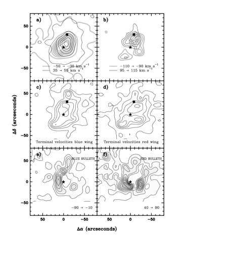
Fig. 3.: a) Spatial distribution of the integrated emission of the $J=2\rightarrow 1$ CO line for blueshifted (solid contours) and redshifted (dashed contours) gas at moderate velocities. The lowest level corresponds to an integrated intensity of 2 K km s^-1; the interval between levels is 20 K km s^-1.
b) Spatial distribution of the integrated $J=2\rightarrow 1$ CO emission for the most extreme velocities of the blueshifted (solid contours) and redshifted (dashed contours) gas. The first level corresponds to 2 K km s^-1 and the interval between levels is 1 K km s^-1. Note that for the most extreme velocities, the blue and red wing CO maxima appear north of IRc2, which does not support the idea of bipolarity around IRc2/I.
c) & d) Spatial distribution of the iso-terminal velocities of the high-velocity gas as measured from the $J=2\rightarrow 1$ CO line corresponding to the blue and red wings respectively. For the blueshifted gas, the first level is $-30\,$km s^-1 and the interval between levels is $-20\,$km s^-1. For the redshifted gas, the first contour level corresponds to 45 km s^-1 and the interval to 20 km s^-1.
e) & f) integrated intensity of the CO $J=2\rightarrow 1$ line emission between $-90$ and $-10\,$km s^-1, and between $40$ and $90\,$km s^-1 for the blue and red HV bullets respectively. The maps have been obtained subtracting a Gaussian profile to the broad line wings (see Rodríguez–Franco et al., 1999). The first contours level is $2\,$K km s^-1, and the interval between levels is $7\,$K km s^-1.
For all the panels, the filled star shows the position of IRc2 and the filled square the position of IRc9.

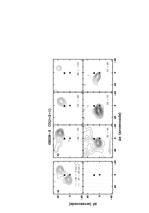
Fig. 4.: a) The upper panel shows the spatial distribution of the fast molecular outflow in Orion–S. The dashed contours show the spatial extension of the $J=2\rightarrow 1$ CO emission for the red wing, and solid contours represent the blue wing. The first level is 9 K km s^-1 and the interval between levels is 2.5 K km s^-1. The lower panel shows the positions where the spectra were taken. The offsets are relative to the FIR 4 ($\alpha(1950)=-5\,^{\rm h}32\,^{\rm m}45.9\,^{\rm s}$, $\delta(1950)=-5^{\rm o}26^{\prime}6^{\prime\prime}$) represented by a filled star. The filled square represents the position of the possible exciting source (see text).
b) Maps of the integrated $J=2\rightarrow 1$ CO emission as a function of the radial velocity in the direction of the Orion$-$SFBO bipolar outflow for the blue (three upper panels) and redshifted (three lower panels) wings. Velocity intervals in  km s^-1 are noted in the lower right corner of every panel. In the velocity intervals between $-20$ and $-80\,$km s^-1 and between 30 and $70\,$km s^-1 the first contour level is 1.4 K km s^-1 and the distance between levels is 0.6 K km s^-1. For the velocity intervals between $-80$ and $-110\,$km s^-1 and between 70 and 90 km s^-1 the first contour level is 1 K km s^-1 and the distance between levels is 0.3 K km s^-1.

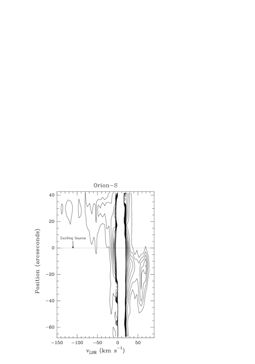
Fig. 5.: Velocity$-$position strip in the direction defined by the symmetry major axis of the Orion$-$SFBO. Vertical scale represents positions relatives to geometric centre of the outflow over the mentioned axis. Dashed horizontal lines are traced in the positions of the exciting source and the 1.3 mm continuous source. The lowest level corresponds to an intensity of 0.13 K; the distance between levels is 0.2 K.

Fig. 6.: The lower panel is a plot of the ratio between the intensity of the CO $J=2\rightarrow 1$ and $J=1\rightarrow 0$ lines. These are shown in the upper and the middle panels, respectively. When the emission is optically thin in both lines this is the opacity ratio. Vertical lines are traced for velocities where the ratios are almost unity. In these positions an increase of the relative intensity of one of the line profiles is shown. The middle panel also shows the recombination line emission H38$\alpha$ (dotted profile).

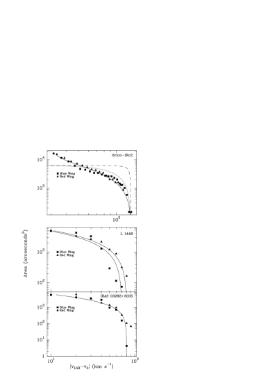
Fig. 7.: a), b), and c) The distribution of the area enclosed by equal projected terminal velocity as a function of the projected terminal velocity for the IRc2, L 1448, and I 3282 bipolar outflows, respectively. For the three panels, the filled squares and filled triangles represents, respectively, the observational data for blue and red line wings. The fits are determined from the model of a jet driven molecular outflow with the parameters in Table 3. This is represented by a solid curve in each panel. In the Orion IRc2 panel we have also represented the expected distribution for an spherical expansion model and an expanding ellipsoid model (dashed line).

Fig. 8.: Panels a) and b): dependence of the mass distribution in velocity intervals of 5 km s^-1 (CO integrated intensity in velocity intervals of 5 km s^-1 wide) with the terminal velocity (distance to the outflow axis) for the IRc2 bipolar outflow. Panel a) corresponds to the blue wing while panel b) to the red wing. In both lobes one can distinguish the region associated to the shock (bow shock) and the region associated to the high-velocity jet. Numbers in the right side of every curve are the value in  km s^-1 of the superior extreme of considered velocity interval.
Panels c), d), e), and f): dependence of the mass distribution in velocity intervals of 10 km s^-1 (CO integrated intensity by velocity interval) with the terminal velocity for the blue (squares) and red (triangles) wings of the L 1448 (panels c) and d)) and I 3282 (panels e) and f))outflows. Panels c) and e) correspond to the region which is far from the exciting source. It is in this region where probably a shock between the ambient gas and the ejected material is produced (bow shock). Panels d) and f) correspond to the most close region to the exciting source. Is in this region where higher terminal velocities are observed. Each curve has been noted with the most negative (blue wing) and most positive (red wing) value in  km s^-1 of the velocity interval considered.

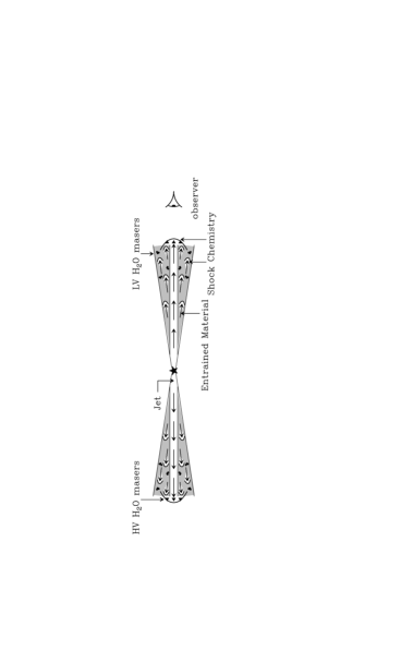
Fig. 9.: A sketch of the proposed model for the IRc2/I outflow. The outflow direction has been rotated by $90^{\rm o}$ with respect the line of sight. The filled star represents the powering source, triangles and dots the high and low velocity H₂O masers respectively and the arrows the direction of the wandering jet in its different episodes. In the head of the jets, bow shocks are represented. It is in these regions where shock chemistry can dominate.

Fig. 10.: Comparison between the blue wing $J=2\rightarrow 1$ CO emission and vibrationally excited molecular hydrogen emission (Beckwith et al., 1978) For each panel, CO emission is represented by continuous contours while H${}_{2}^{*}$ is represented by dashed contours. Left and right panels show the positions noted as Pk1 and Pk2 by Beckwith et al. (1978). In these panels, emission corresponding to the largest velocities are represented (left, blue and right, red). Also positions of HV water masers are noted (squares represent negative velocities or blueshifted, while triangles represent positive velocities or redshifted). Velocity intervals of integration appear in the bottom right corner. First level is 1 K km s^-1 and interval between levels is 0.5 K km s^-1. The CO emission in central panel represents the addition of the emissions between $-100$ and $-30\,$km s^-1 plus 45 and 95 km s^-1. First level is 15 K km s^-1 and interval between levels is 15 K km s^-1. For all the panels the filled star represents the IRc2 position.

References

- 1 Anglada, G., et al.: 1998, AJ 116, 2953.
- 2 Bachiller, R., Cernicharo, J.: 1990, A&A 239, 276.
- 3 Bachiller, R., Cernicharo, J., MartínPintado, J., Tafalla, M., Lazareff, B.: 1990, A&A 231, 174.
- 4 Bachiller, R., MartínPintado, J., Planesas, P.: 1991, A&A 251, 639.
- 5 Bachiller, R., Pérez–Gutiérrez, M.: 1997, ApJ 487, L93.
- 6 Beckwith, S., Persson, S.E., Neugebauer, G., Becklin, E.E.: 1978, ApJ 223, 464.
- 7 Boreiko, R.T., Betz, A.L.: 1989, ApJLet 346, L97.
- 8 Boreiko, R.T., Betz, A.L., Zmuidzinas, J.: 1989, ApJ 337, 332.
- 9 Brand, P.W.J.L., Moorhouse, A., Burton, M.G., Geballe, T.R., Bird, M., Wade, R.: 1988, ApJLet 334, L103.
- 10 Cabrit, S.: 1995, Atrophysics and Space Science 233, 81.
- 11 Chernin, L.M., Masson, C.R., Gouveia dal Pino, E.M., Benz W.: 1994, ApJ 426, 204.
- 12 Chernin, L.M., Masson, C.R.: 1995, ApJ 455, 182.
- 13 Chernin, L.M., Wright, M.C.H.: 1996, ApJ 467, 676.
- 14 Doeleman, S.S., Londsdale, C.J., Pelkey, S.: 1999, ApJLet 510, L55.
- 15 Doyon, R., Nadeau, D.: 1988, ApJ 334, 883.
- 16 Erickson, N.R., et al.: 1982, ApJLet 261, L103.
- 17 Fuente, A., Martín–Pintado, J., Rodríguez–Franco, A., Moriarty-Schieven, G.D: 1998, A&A 339, 575.
- 18 Garden, R., Geballe, T.R., Gatley, I., Nadeau, D.: 1986, MNRAS 220, 203.
- 19 Gaume, R. A., Wilson, T.L., Vrba, F.J., Johnston, K.J., Schmid–Burgk, J.: 1998, ApJ 493, 940.
- 20 Geballe, T.R., Persson, S.E, Simon, T., Lonsdale. C.J., McGregor, P.J.: 1986, ApJ 302, 693.
- 21 Genzel, R., Downes, D.: 1983, en “Highlights of Astronomy”, ed. R. West, p.689, Dordrecht: Reidel.
- 22 Goldsmith, P.F., et al.: 1981, ApJLet 243, L82.
- 23 Graf, U.U., Genzel, R., Harris, A.I., Hills, R.E., Russell, A.P.G., Stutzki, J.: 1990, ApJ 358, L49.
- 24 Greenhill, L.J., Gwinn, C.R., Schwartz, C., Moran, J.M., Diamond, P.J.: 1998, Nature 396, 650.
- 25 Gueth, F., Guilloteau, S., Bachiller, R.: 1996, A&A 307. 891.
- 26 Johnston, K.J., Gaume, R., Stolovy, S., Wilson, T.L., Walmsley, C.M., Menten, K.M.: 1992, ApJ 385, 232.
- 27 Keene, J., Hildebrand, R.H., Whitcomb, S.E.: 1982, ApJLet 252, L11.
- 28 Li, Z.Y., Shu, F.H.: 1996, ApJ 468, 261.
- 29 MartínPintado, J., Bachiller, R., Fuente, A.: 1992, A&A 254, 315.
- 30 MartínPintado, J., RodríguezFranco, A.: 2000, in preparation.
- 31 Nadeau, D., Geballe, T.R.: 1979, ApJLet 230, L168.
- 32 Phillips, T.G., Huggins, P.J., Neugebauer, G., Werner, M.W.: 1977, ApJLet 217, L161.
- 33 Plambeck, R.L., Snell, R.L.: 1995, ApJ 446, 234.
- 34 Plambeck, R.L., Wright, M.C.H., Welch, W.J., Bieging, J.H., Baud, B., Ho, P.T.P., Vogel, S.N.: 1982, ApJ 259, 617.
- 35 Plambeck, R.L., Snell, R.L., Loren, R.B.: 1983, ApJ 266, 321.
- 36 Raga, A.C., Biro, S.: 1993, MNRAS 264, 758
- 37 Raga, A.C., Cabrit, S.: 1993, A&A 278, 276.
- 38 RodríguezFranco, A., MartínPintado, J., Wilson, T.L.: 1999, A&A 344, L57.
- 39 Scoville, N.Z., Hall, D.N.B., Kleinmann, S.G., Ridway, S.T.: 1982, ApJ 253, 136.
- 40 SchmidBurgk, J., Güsten, R., Mauersberger, R., Schulz, A., Wilson, T.L.: 1990, ApJLet 362, L25.
- 41 Snell, R.L., Scoville, N.Z., Sanders, D.B., Erickson, N.R.: 1984 ApJ 284, 176.
- 42 Stahler, S.W.: 1994, ApJ 422, 616.
- 43 Van Vliet, A.H.F., de Graauw, T., Lee, T.J., Lidholm, S., Stadt, H.v.d.: 1981, A&A 101, L1.
- 44 Wannier, P.G., Phillips, T.G.: 1977, ApJ 215, 796.
- 45 Wilson, T.L., Serabyn, E., Henkel, C.: 1986, A&A 167, L17.
- 46 Wright, M.C.H., Plambeck, R.L., Mundy, L G.; Looney, L.W.: 1995, ApJLet 455, L185.
- 47 Wright, M.C.H., Plambeck, R.L., Wilner, D.J.: 1996, ApJ 469, 216.
- 48 Zuckerman, B., Kuiper, T.B.H., RodríguezKuiper, E.N.: 1976, ApJLet 209, L137.
- 49 Ziurys, L.M., Martin, R.N., Pauls, T.A., Wilson, T.L.: 1981, A&A 104, 288.
- 50 Ziurys, L.M., Friberg P.: 1987 ApJLet 314, L49.