The High-Resolution OTF Survey of the ${}^{12}CO$ in M 31

Abstract

We are performing a fully sampled survey of the ¹²CO(1-0) line emission of the nearby galaxy M 31 with the IRAM 30-m telescope. The resolution obtained is $23^{\prime\prime}$ which corresponds to about 90 pc along the major axis. This small beam is well adapted to the size of typical structures of the molecular gas and allows to detect even interarm cloud complexes. We chose an on-the-fly observing technique which allows us to cover the large area of about 1 square degree in a reasonable time.

Until now, almost three quarters of the galaxy have been observed in the (1-0) line and some selected regions with a longer integration time in the (2-1) transition as well. Compared to the Hi emission, the spiral arms show a higher contrast and more structure, albeit the general morphology is very similar. A first analysis suggests that the CO emission is a very good tracer of the molecular gas in M 31. In addition to the survey, we perform observations of selected complexes down to the sub-arcsecond level with the IRAM interferometer. Together with data of other species such as dust or neutral carbon we hope to proceed towards a better understanding of the molecular gas at large and small scales.

Radioastronomisches Institut der Universität Bonn (RAIUB), Germany

in collaboration with

1. Introduction

The investigation of the large-scale conditions for the star formation is an important problem of modern astronomy. The final stage of the process is reached when individual regions within diffuse molecular clouds start to coagulate into dense, gravitationally bound complexes that eventually collapse and form stars. The trigger to start such a contraction is however unknown, and in particular the influence of large-scale phenomena on this process is unclear. Possible candidates are cloud-cloud collisions (e.g. due to orbit crowding), MHD shocks (caused by density waves), ‘contagious’ star formation induced by supernova blast waves or thermal and magnetic instabilities. The relative importances of these processes are however uncertain and the time scales are unknown.

The small-scale properties of star-forming clouds are studied in great detail in the Milky Way, but there are severe difficulties to obtain good information about the large-scale structure. This is of course due to our position within the disk of the Galaxy, but also because of the problem to determine proper distances. We thus have to investigate an external galaxy and the obvious choice is the Andromeda Galaxy, M 31. It is rather close, at a well determined distance (784 kpc after Stanek & Garnavich 1998), its properties are similar to that of our Milky Way and a wealth of observations at all wavelengths is available for comparisons. In particular, a complete survey of the $\lambda$ 21 cm line emission of the atomic hydrogen has been performed with the WSRT at $24^{\prime\prime}\times 36^{\prime\prime}$ angular resolution (Brinks & Shane 1984).

Several attempts have been made to observe the emission of the CO in that galaxy in order to investigate the properties of the molecular gas, but this turned out to be unexpectedly difficult. Early attempts (e.g. Combes et al. 1977) resulted in a rather high number of non-detections – only the dustiest regions showed a reasonable probability to detect molecular gas (e.g. Lada et al. 1988, Ryden & Stark 1986). Such a sample is however biased, of course, and only a survey with uniform coverage can give the necessary information about the large-scale properties. The first complete survey of M 31 was however published only a few years ago (Dame et al. 1993) and had an angular resolution of $9^{\prime}$ (2 kpc along the major axis).

2. Observations

2.1. Preparatory Studies

In 1993, we made a new attempt to study the properties of an unbiased sample of molecular clouds and chose the target region on kinematical grounds only: we focused on a place where the major axis is crossed by a spiral arm whose location was determined by a kinematical analysis of the Hi data (Braun 1991). The observations were performed with the IRAM 30-m telescope in a standard “on-off” observing mode. At a distance of about $38^{\prime}$ south-west from the center, CO emission was indeed clearly detected around the major axis and subsequently an area of about $3^{\prime}\times 4^{\prime}$ was mapped. We found an extended cloud complex and several individual clumps within this area. The properties of the clouds varied substantially within these few arcminutes, e.g. we observed line widths from FWHM 20 km s^-1 down to only 4 km s^-1. The line temperatures found were of the order of 0.1 to 0.4 K (in T${}_{A}^{*}$ units) – and not limited to only about 20 mK as found by Dame et al. (1993).

The results showed clearly that the CO emission of M 31 is highly clumped and the low intensities of the CfA survey are caused by the small filling factor of the $9^{\prime}$ beam. A high spatial resolution is thus mandatory to reveal the properties of the molecular gas. This is however a difficult task because of the size of the emission area: a surface of about 1 square degree has to be mapped with an angular resolution of less than half an arcminute. The sensitivity should reach 0.2 K or better at a velocity resolution of a few km s^-1.

In principle, there are at least two ways to substantially speed up the imaging speed compared to the classical on-off mode: one could use multiple-beam receivers and thus cover a larger field with every “on”-position or use a continuous scanning which reduces overlays for telescope moving and reference positions by a very large amount.

2.2. Observation technique

Based on the experience obtained with the little map and the various already published results we choose an “OTF” (On-The-Fly) observing technique for our survey. Here, the telescope is moved across the source at a constant speed, taking data at a high rate, so that there is a sufficient number of dumps within the diameter of the beam. In our case, we use a scanning speed of $4^{\prime\prime}$/second and take a dump every second, which ensures a good sampling of the $22^{\prime\prime}$ beam. The field is covered by adding subsequent scans parallel to the first at a small distance, in our case $8^{\prime\prime}$. The orientation of the scans is defined in a coordinate system fixed to the center of the source; on the sky, the scans therefore remain equidistant and the individual dumps equally spaced within the tracking errors of the telescope ($\ll 1^{\prime\prime}$ during a normal scan). That way, the coverage thus obtained is uniformly and densely sampled.

The reference data are obtained before and after each scan at positions free of emission; typically, we integrated 30 seconds there, so that the noise of this data is significantly lower than the noise of the dumps along the scan. A scan of a length of $20^{\prime}$ lasts five minutes given the parameters above, so a complete sequence (calibration – reference – scan – reference) takes about 6.5 minutes to complete. In order to obtain the sensitivity needed, two SIS receivers are used in parallel which look at the same sky position. Moreover, each field is scanned twice, in orthogonal orientations. That way, we are able to obtain a sensitivity of $\sim 0.15$ K or better in the final map (T${}_{A}^{*}$ scale).

The orthogonal orientation of the second coverage not only results in a dense sampling of the source area, but allows for a special data reduction technique that supresses so-called “scanning noise”. It is derived from the “basket-weaving” method presented by Emerson & Gräve (1988) for cm continuum observations and adapted to line observations by P. Hoernes (1998). A short overview of the procedure is given below in Sect. 2.3.. As a result, the noise distribution is very smooth and in particular we avoid spurious elongated artifacts.

The main backends used are filterbanks with 1 MHz resolution. Three units are available at the 30-m telescope: two of them offer 256 channels and one 512 channels. The total bandwidth of the receivers and the IF system being 500 MHz each, the necessary velocity coverage for M 31 is thus easily obtained with a sufficient resolution (2.6 km s^-1). The 512-channel filterbank and the autocorrelators also available at the telescope were used for the two 230 GHz receivers that run in parallel to the 115 GHz units. Each point may thus be observed with up to four receivers simultaneously – but for proper observations at the higher frequency the observational parameters have to be adapted to the smaller beam, of course.

2.3. Data reduction

The observation method results in separate files for the calibration, the reference and the source data. The first step in the data reduction process is thus to apply the appropriate calibration to each dump. Thereafter, the spectrum at the reference position is subtracted from the source points. Various averaging options for the case of multiple references are available, but a straight mean of the values obtained before and after the individual scan is usually sufficient. After this subtraction, we have a set of spectra comparable to the usual output of “on-off” or wobbler techniques, with one second of integration time per spectrum.

The next step in the data reduction is the subtraction of spectral baselines and the removal of erroneous data points. Such points are e.g. introduced by bad channels in the filterbanks. They are relatively easy to detect due to their “singular” nature and the occurrence at the same channel in independent spectra. The fitting of the baseline needs a bit more thought: since each scan contains several hundred spectra, we need a routine that is able to determine the necessary line windows by itself. Here, we profit largely from the WSRT Hi data that have a resolution comparable to our survey ($24^{\prime\prime}\times 36^{\prime\prime}$, Brinks & Shane 1984). We assume that the velocity structure of the atomic gas (Hi) is similar to that of the molecular gas (CO). Then, we can use the kinematical information in the Hi-data to determine the velocity interval possibly containing CO emission and fit the spectral baseline to the data outside of this region. In the case of M 31 this is a very safe procedure because the CO emission is weak and even a possible error in the line window does not change the fit of the baseline very much. In any case, the baseline fit is a linear procedure and may be used iteratively, if necessary.

Now it is time to actually ‘reduce’ the data – remember that we still are working on a $4^{\prime\prime}\times 8^{\prime\prime}$ data grid for the $22^{\prime\prime}$ beam. We thus  bf regrid the data onto a convenient regular grid, which at the same time allows to correct for tracking errors and to introduce additional scans (e.g. to back up single lines with higher noise). It may be advisable, however, to maintain the distance between individual scans in the grid setup for the next step of the data reduction.

At this stage, we combine several maps (which are actually data cubes) using the “basket-weaving” method already mentioned above (Emerson & Gräve 1988). Inspection of the maps shows that quite often drifts of the zero level are remaining even after the subtraction of a spectral baseline. Adjacent scans thus may show a different value for neighboring points (at a distance of $8^{\prime\prime}$ compared to a beam of $22^{\prime\prime}$) because they have been observed through a different atmosphere, separated in time by e.g. six minutes (see Fig. 1 upper left). Now remember that we have scanned the area of interest at least twice, at orthogonal orientations. Thus, we have two data sets where the distribution of coherent dumps (along the scan) and incoherent dumps (in different scans) is orthogonal.

In the two-dimensional frame of a map, the scans constitute regularly spaced rows or columns. Any feature that occurs with such a fixed period (e.g. a varying zero level in each scan) will be projected into a very narrow interval by a 2-D Fourier transform (Fig. 1, upper right). Thus, it is easy to apply a filter function to suppress this noise contribution. The orientation of this interval depends of course on the original scanning direction, so the part taken out can be reconstructed from the other input maps. This also avoids unwanted filtering of linear source structures, because a priori only periodic arrangements are filtered – and only in one specific orientation per input frame.

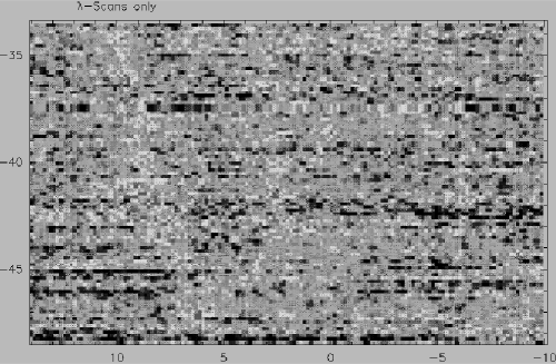
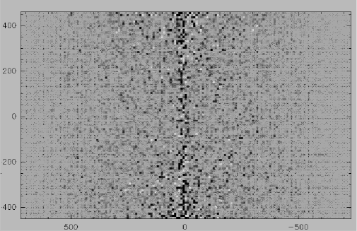
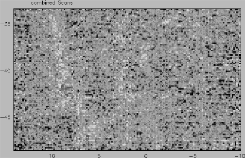
Figure 1.: Example of the FFT filtering: in the upper row a raw image is shown, scanned in one direction only (left), together with its Fourier transform (right). The stripes are transformed into a very narrow strip which is weighted down. To the left, the result of the filtering and combination is given. Only random noise remains.

After the filtering, the input maps are coadded – in principle, any number of coverages with arbitrary scanning orientations can be used as input. If the coverage should be not the same for all input maps, the quality of the noise filtering will vary over the combined area, of course. However, the procedure is rather ‘friendly’ and does not introduce edge-effects at the borders of the individual coverages. For spectral data, each spectral channel is treated as an individual map. The whole procedure works on the data pixels and it is up to the user to ensure a coherent data set beforehand.

Until now, the pixels are coherent only at the level of the gridding, which is typically of the order of half a beam width or less. Hence, we smooth the data as the last step of the data reduction. The smoothing gaussian is chosen small enough in order not to degrade the original resolution (we obtain a final resolution of $23^{\prime\prime}$); this leaves the source structures untouched, but further suppresses the random noise in the pixels.

3. Results

3.1. The map

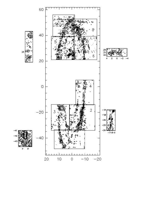
Figure 2.: Overview of the mapped regions as of summer ‘99. The coordinates are fixed at the center of M 31 (R.A._B1950.0 $0^{h}40^{m}00.3^{s}$, Dec._B1950.0 $41^{\circ}00^{\prime}03^{\prime\prime}$); X is positive towards the NE along the major axis (P.A. $37.7^{\circ}$), Y is positive to the SE along the minor axis. The smaller fields show selected regions that have been mapped with a full sampling in the (2-1) line as well. Note that part of the data in the northern part is still preliminary and the contours have been chosen such as to show some effects of the scanning noise.

Until now, about three quarters of M 31 have been mapped with full sampling for the $22^{\prime\prime}$ beam at the ¹²CO(1-0) line transition (see Fig. 2). In addition, we choose several regions with particular properties and observed them in a mode adapted to fully sample the smaller beam at the (2-1) transition (shown in the fields surrounding the main frame in Fig. 2).

Over most of the area surveyed so far, coherent spiral arm pieces are clearly visible. The arm/interarm contrast is high, but there are small cloud complexes scattered over a large part of the surface. Note however, that only in the southern half of the map the lowest contour is at least $3\sigma$, whereas in the northern part the data was still preliminary at the time of the conference. There, the contours have been chosen such as to show the effects of the scanning procedure which result e.g. in the horizontal stripes at the upper end of fields 7 and 8. In any case, we check such weak points with dedicated on-off measurements and maintain only those that can be confirmed – which is usually the case.

3.2. Comparisons with other data and first results

There is a wealth of observations available for M 31, covering the whole wavelength range. As described above, we used the Hi data cube of the WSRT survey (Brinks & Shane 1984) already for the determination of the line windows during the data reduction. Now, we can compare the two data sets to obtain a picture of the properties of the atomic vs. the molecular gas. The molecular gas turns out to show a significantly higher contrast, but the general structure is very similar to that of the atomic gas: the main emission is found in a “ring” and very few gas can be found close to the center. The ratio of molecular/atomic gas decreases with radius, but individual molecular complexes have nevertheless been found out to a distance of about 18 kpc. The kinematical signature is rather similar for both kinds of gas, which justifies the use of the Hidata in the baseline fitting procedure.

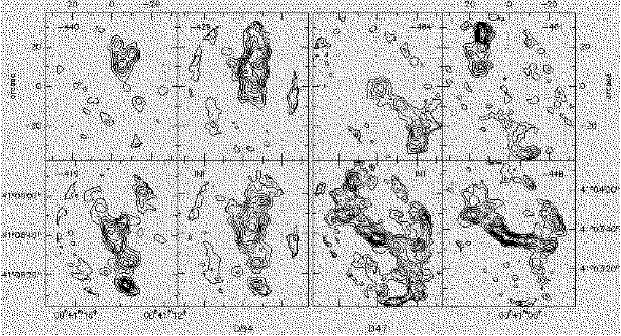
Figure 3.: An example of two cloud complexes with different properties, observed with the PdB interferometer. The left half shows the quiescent complex D84, the right half the disturbed region D47. The two lower inner panels (labeled ‘INT’) give the integrated emission, whereas the outer panels show the structure in selected velocity bins, labeled with the central velocity. Note the absence of emission at the central position of D47 in the $-461$ km/s channel; the corresponding spectrum is double-peaked with a 40 km/s wide gap.

Large-scale streaming motions are not prominent along the spiral arms – the data are rather dominated by local effects. They show up as double- or multiple-peaked spectra with total widths of up to 50 km s^-1 (cf. Fig. 3). A comparison with the distribution of ionized regions (Devereux 1994) suggests a relation between such disturbed molecular clouds and the Hii regions (see Fig. 2 of Neininger et al. 1998) for the region presented in Fig. 3).

4. Summary

Technical items

The OTF method is a fast, flexible and versatile observing mode which yields high-quality data. Longer integration times per point can be achieved by co-adding a corresponding number of coverages. In principle, it can be adapted to all mapping projects with single-dish telescopes – the limitations are usually technical, such as receiver stability, maximum telescope speed, maximum dump rate or data storage capacity. Our setup allows us to map an area of 10 arcmin² at a typical noise of 150 mK per spectrum in 1 hour of telescope time. Using specially designed filtering techniques, spurious features can be removed and a homogeneous result can be achieved – even in wavelength bands that are seriously affected by atmospheric effects.

Astronomical results

The molecular gas in M 31 has a high arm/interarm contrast, but single cloud complexes are found between the arms. The spatial filling factor is rather low. The bulk of the molecular gas is situated between a radius of about 4 kpc and 13 kpc, but some cloud complexes have been observed out to distances of 18 kpc. The total gas mass (Hi + H₂) corresponds well to the optical extinction. The signature of a possible density wave is very weak in the molecular gas, instead it seems to be dominated by local effects.

Acknowledgments.

Special thanks to the IRAM staff which has made the OTF observations possible – in particular to A. Sievers, W. Brunswig, W. Wild and the receiver engineers. Of special importance were some hydrogen data: we thank E. Brinks and R. Braun for the Hi cubes and N. Devereux for his H$\alpha$ image.

References

Braun, R. 1991, ApJ, 372, 54

Brinks, E., & Shane, W.W. 1984, A&ASup., 55, 179

Combes, F., Encrenaz, P.J., Lucas, R., & Weliachew, L. 1977, A&A, 61, L7

Dame, T., et al. 1993, ApJ, 418, 730

Devereux, N.A., Price, R., Wells, L.A., & Duric, N. 1994, AJ, 108, 1667

Emerson, D.T., & Gräve, R. 1988 A&A, 190, 353

Hoernes, P. 1998, PhD Thesis, University of Bonn

Lada, C.J., et al., 1988, ApJ, 328, 143

Neininger, N., Guélin, M., Ungerechts, H., Lucas, R., & Wielebinski, R. 1998, Nature, 395, 871

Ryden, B.S., & Stark, A.A., 1986, ApJ, 305, 823

Stanek, K.Z., & Garnavich, P.M. 1998, ApJ, 503, L131