Multifrequency Observations of Giant Radio Pulses from the Millisecond Pulsar B1937+21

Abstract

Giant pulses are short, intense outbursts of radio emission with a power-law intensity distribution that have been observed from the Crab Pulsar and PSR B1937$+$21. We have undertaken a systematic study of giant pulses from PSR B1937$+$21 using the Arecibo telescope at 430, 1420, and 2380 MHz. At 430 MHz, interstellar scattering broadens giant pulses to durations of $\sim 50~{}\mu$secs, but at higher frequencies the pulses are very short, typically lasting only $\sim 1$–$2~{}\mu$secs. At each frequency, giant pulses are emitted only in narrow ($\mathrel{\hbox to0.0pt{\lower 3.0pt\hbox{$\mathchar 536\relax$}\hss}\raise 2.0pt\hbox{$\mathchar 316\relax$}}10~{}\mu$s) windows of pulse phase located $\sim 55$–$70~{}\mu$sec after the main and interpulse peaks. Although some pulse-to-pulse jitter in arrival times is observed, the mean arrival phase appears stable; a timing analysis of the giant pulses yields precision competitive with the best average profile timing studies. We have measured the intensity distribution of the giant pulses, confirming a roughly power-law distribution with approximate index of $-1.8$, contributing $\mathrel{\hbox to0.0pt{\lower 3.0pt\hbox{$\mathchar 536\relax$}\hss}\raise 2.0pt\hbox{$\mathchar 318\relax$}}0.1\%$ to the total flux at each frequency. We also find that the intensity of giant pulses falls off with a slightly steeper power of frequency than the ordinary radio emission.

1 Introduction

Despite their remarkable frequency stability, most radio pulsars exhibit considerable pulse-to-pulse intensity fluctuations. A histogram of the pulse intensity typically shows a roughly exponential or Lorentzian shape (e.g., Manchester & Taylor (1977)), with a tail extending out to perhaps ten times the mean pulse strength.

The Crab pulsar (PSR B0531+21), by contrast, exhibits frequent, very strong radio pulses extending to hundreds of times the mean pulse intensity (e.g., Lundgren et al. (1995)). These so-called “giant pulses” exhibit a characteristic power-law intensity distribution—a phenomenon that for many years was observed in no other pulsar. Despite hints from early observations (Wolszczan, Cordes, & Stinebring (1984)), it came as a surprise to find qualitatively similar behavior from PSR B1937$+$21, the first (and still fastest known) millisecond pulsar (Sallmen & Backer (1995); Cognard et al. (1996)).

The Crab pulsar and PSR B1937$+$21 could hardly be less similar in their properties. The Crab pulsar, born in A.D. 1054, is the youngest known pulsar, and B1937+21 is one of the oldest, with a characteristic spin-down age of $\sim 2\times 10^{8}$ yrs. The inferred surface magnetic field strength of the Crab pulsar, $B=4\times 10^{12}$ G, is about $10^{4}$ times as high as that of B1937+21. Although the Crab is the fastest of the high field pulsars, with a period of $P=33$ ms, it is twenty times slower than the 1.56 ms B1937+21. The pulsars’ only identified common feature is their similarly strong magnetic field strength at the velocity-of-light cylinder, $\sim 10^{6}$ G, which is higher than that for any other known pulsar (Cognard et al. (1996)). Whether this is coincidence, or in some way responsible for the observed giant pulse behavior, is unknown.

All previous studies of giant pulses from B1937+21 have been at or near 430 MHz with the exception of some limited, inconclusive data at 1.4 GHz (Wolszczan et al. 1984). We present below the first multifrequency study of giant pulses in B1937+21. In §2, we describe the observations and giant pulse search algorithms. A comparison of the arrival times of normal and giant pulse emission is discussed in §3. Following this, we discuss pulse morphology in §4 and the limits of accurate timing in §5. Using the arrival data, we present intensity distributions of the giant pulses and the contaminant noise in §6. In §7, we discuss the approximate spectrum of the largest giant pulses. Finally, in §8, we point to open questions and necessary future observations.

2 Observations and Signal Processing

All observations were made using the Princeton Mark IV instrument (Stairs et al. (1999)) at the 305 m Arecibo telescope, between 1998 February 21 and 1999 August 1. Observations were made at three frequencies, as part of an ongoing timing study of this pulsar. The pulsar signal strength varied because of interstellar scintillation; observations made during times of strong signal were retained for the giant pulse analysis. The data used for this work included 30 minutes ($\sim 10^{6}$ pulses) at 430 MHz, 4 hours ($\sim 10^{7}$ pulses) at 1420 MHz, and 26 minutes ($\sim 10^{6}$ pulses) at 2380 MHz.

After completion of the observations, the data were coherently dedispersed in software by convolution with a complex chirp function (Hankins & Rickett (1975)), to remove the progressive phase delays as a function of frequency caused by free electrons in the interstellar medium (ISM). The analysis pipeline has been described by Stairs et al. (1999). At the dispersion measure of PSR B1937$+$21(71), with a 10 MHz bandwidth, the dispersive smearing at 430 MHz, 1420 MHz, and 2380 MHz totals 74.16 ms, 2.06 ms, and 0.44 ms, respectively, before coherent dedispersion. After dedispersion, the signals from the two orthogonal polarizations were squared and cross multiplied to produce the four Stokes parameters. Because we were analyzing data taken primarily for other purposes, in most cases insufficient calibration data were available for high precision polarization calibration. We therefore concentrate on analysis of the total intensity data.

After coherent dedispersion, the standard timing analysis pipeline was used to fold the data synchronously with the known topocentric period of PSR B1937$+$21, to produce average profiles. In a parallel analysis, the data were searched for strong individual pulses. Initial exploratory analysis confirmed that all strong pulses were confined to fairly narrow windows on the tails of the main pulse (MP) and interpulse (IP). At 430 MHz, giant pulses were therefore identified as in Cognard et al. (1996), by measuring the integrated flux density in 150$~{}\mu$sec windows located on the tails of the MP and IP. At higher frequencies, where the giant pulses were much narrower (many lasting only a few $0.1$–$0.2~{}\mu$sec bins) and appeared in a region of pulse phase that was significantly wider than the individual pulses, giant pulses were identified by searching for pairs of bins with combined energy greater than a threshold level. Because of the relative computational efficiency of this procedure, we did not limit our search to particular regions of pulse phase. But as at 430 MHz, giant pulses were only detected in the tails of the MP and IP. (Note that this appears to be in conflict with the results of Wolszczan et al. (1984).)

Interstellar scintillation strongly modulated the apparent intensity of the pulsar signal from day to day. Scintillation should affect the normal and giant pulse emission identically. Therefore, in order to compare giant pulse intensities observed on different dates, we accounted for these variations by calibrating the average normal emission flux density for each run to the power-law model given by Foster, Fairhead, and Backer (1991). They found that the flux density as a function of frequency could be expressed as $F$[mJy]$=(25.9\pm 2.6)\,\nu^{-2.60\pm 0.05}$, where $\nu$ is in GHz. We use units of [Jy] for flux density and [Jy$\cdot\mu$sec] for integrated flux density.

3 Giant pulse distribution in time and pulsar phase

An important difference between giant pulses in the Crab pulsar and in PSR B1937$+$21 appears in the distribution of the pulses with respect to the star’s rotational phase. Individual Crab giant pulses arrive at phases distributed throughout most of the emission envelope of the normal pulse profile. In contrast, the early observations of giant pulses from B1937+21 at 430 MHz found that they arrived only in narrow regions on the tails of the two normal pulse components (Backer (1995); Cognard et al. (1996)). With our greater sensitivity, we confirm this result at 430 MHz and find the same behavior at 1420 and 2380 MHz.

Figures 1–3 show the average flux due to all giant pulses as a function of pulse phase along with the average normal emission. For each run, giant pulses were selected using an intensity threshold chosen to minimize noise contamination. As is clear from these figures, the giant pulses occur well after the normal emission phase; in particular the giant pulses do not produce the “notch” emission on the trailing edge of the MP as had been speculated by Cognard et al. (1996).

To characterize the average properties of the giant pulse emission, we have fit the average giant pulse profile at each frequency with a Gaussian model at 2380 and 1420 MHz and, to account for interstellar scattering, with a model consisting of a Gaussian convolved with an exponential tail at 430 MHz. We find best-fitting Gaussian widths (FWHM) of 3$~{}\mu$s (4$~{}\mu$s) for the MP (IP) giant pulse profile at 2380 MHz and 4.3$~{}\mu$s (4.1$~{}\mu$s) for the MP (IP) giant pulse profile at 1420 MHz. At 430 MHz, we find that the MP and IP giant pulse profiles can be adequately described as Gaussians with widths 6.6$~{}\mu$s and 6.4$~{}\mu$s, respectively, convolved with an exponential scattering tail with $\tau=28~{}\mu$s. This scattering timescale $\tau$ is similar to that estimated from measurements of the normal profile, confirming that the structure observed in the low frequency average giant pulse profile is dominated by propagation effects. (Because our exponential scattering model is probably an oversimplification of the true effects of scattering on the signal (e.g., Sallmen et al. (1999)), our estimates of the intrinsic width of the mean giant pulse profile at 430 MHz should be considered an upper limit.)

At high frequency, the windows in which giant pulse emission occur are much narrower than the average pulse emission windows. Indeed, they are remarkably narrow both absolutely and as a fraction of the pulsar period, each corresponding to less than one degree of rotational phase. They are, we believe, the sharpest stable features ever detected in a pulsar profile. It is this property that makes the mean giant pulse emission from PSR B1937$+$21 a potentially valuable fiducial point for high-precision timing observations, as discussed in §5 below.

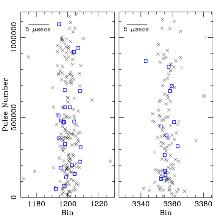
Figure 4: Distribution of giant pulses at 1420 MHz (on MJD 50865) with integrated flux density $\geq 30~{}$Jy$\cdot\mu$secs, in both pulse phase (1 bin $\simeq 0.38~{}\mu$secs) and pulse number. Arrival uncertainty for any given giant pulse is $\lesssim 0.5~{}\mu$sec. The left panel shows the MP region, the right panel the IP region. In each region, the pulses are confined to a very narrow window—10 bins (of 4096 total) corresponds to about $0.9^{\circ}$ of pulse phase—and have a temporal distribution consistent with a Poisson process. The same is true for a subset of the strongest giant pulses, with integrated flux density $\geq 80~{}$Jy$\cdot\mu$secs, which are indicated with open squares.

We have also investigated the distribution of giant pulses over time, finding consistency with Poisson statistics (so neighboring giant pulses appear uncorrelated). The distribution in time during one observation is illustrated in Fig. 4, which displays all pulses with integrated flux density $\geq 30~{}$Jy$\cdot\mu$secs. Also shown are the brightest pulses, with integrated flux density $\geq 80~{}$Jy$\cdot\mu$secs. The arrival time uncertainty for any given giant pulse is $\lesssim 0.5~{}\mu$secs; this will be discussed further discussed in §4. We find no difference in the distributions of the more powerful and less powerful giant pulses, except for rate. The giant pulse distribution also appears very stable over this half-hour scan, with no apparent drifting or nulling periods, although the density drops off slightly at the end of the scan, especially in the IP, as interstellar scintillation reduces the mean pulsar flux relative to our threshold values.

4 Individual Pulse Morphology

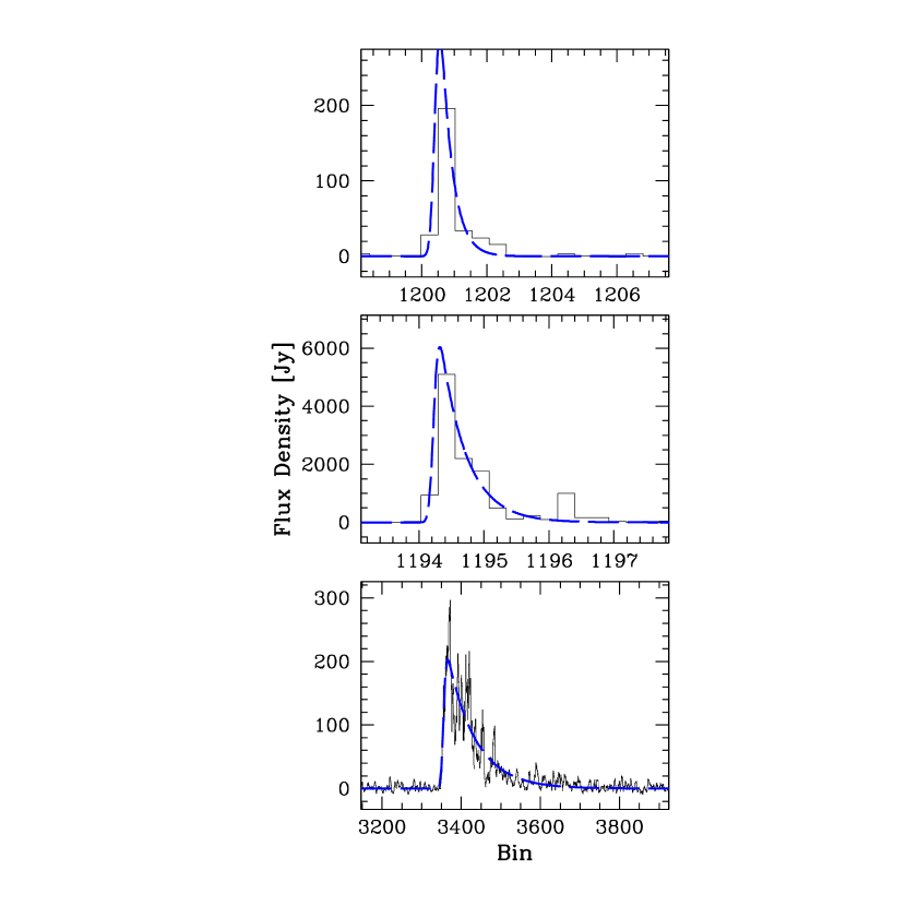
Figure 5: Strongest individual giant pulses at 2380 (top), 1420 (middle), and 430 (bottom) MHz. Flux density (solid) and fitted convolved Gaussians (long-dash) are shown. Each bin corresponds to $\sim 0.38~{}\mu$secs. The sampling interval for the top and bottom plots is $0.2\,\mu$secs, and for the middle plot it is $0.1\,\mu$secs. The 430 MHz data has been boxcar smoothed by 8 data points.

The average giant pulse profiles constrain the properties of the giant pulse emission region. Also of interest are the properties of individual giant pulses, which constrain the giant pulse emission mechanism itself. To study individual giant pulses, which are narrower than the mean giant pulse envelope, we must account for scattering effects even at frequencies above 430 MHz. As discussed above, scattering by a thin turbulent screen degrades a signal by effectively convolving it with a one-sided exponential tail. (Although more sophisticated models of the ISM will have more complex effects on the observed signal, we find the simple thin-screen model adequately describes the vast majority of giant pulses we have observed.) We have fit all candidate giant pulses with a Gaussian, $A\,\mbox{exp}\{-(t-t_{0})^{2}/(2\sigma^{2})\}$, convolved with an exponential tail, $e^{-t/\tau}/\tau$, with four fit parameters, $A$, $t_{0}$, $\sigma$, and $\tau$. Shown in Fig. 5 are the strongest giant pulses found at each frequency along with their fitted convolved Gaussians.

After visually inspecting many giant pulses at all three frequencies, we see no evidence for intrinsic multiple-peaked emission, which contrasts with giant pulses observed from the Crab pulsar (Sallmen et al. (1999)). Although receiver noise dominates the profiles, most pulses show a fast rise followed by an exponential decay, consistent, on average, with scattering. We have more quantitatively verified our model for the pulse morphology by cross correlating all of the giant pulses with a standard giant pulse, shifting by the lag which maximizes the cross correlation (to correct for the observed pulse-to-pulse jitter), then folding. For any choice of the standard giant pulse, this has always produced a single-peaked, short-rise-time, exponential-decaying profile, which, itself, is well fit by our model. Gaussian widths (FWHM) of $6$, $0.2$, and $0.2~{}\mu$secs and scattering timescales of $\tau\simeq 29$, $0.2$, and $0.2~{}\mu$secs were determined at 430, 1420, and 2380 MHz, respectively, for both the MP and IP shifted, folded giant pulse profiles. As previously mentioned in §3, our exponential scattering model is probably an oversimplification of the true effects of scattering, implying that our estimates should be considered upper limits.

Table Multifrequency Observations of Giant Radio Pulses from the Millisecond Pulsar B1937+21 lists the range of scattering timescales, $\tau$ [$\mu$sec], found at each frequency. Overall, we find the following ranges: $\tau\simeq 13$–$40~{}\mu$s (430 MHz), $\tau\mathrel{\hbox to0.0pt{\lower 3.0pt\hbox{$\mathchar 536\relax$}\hss}\raise 2.0pt\hbox{$\mathchar 316\relax$}}1.1~{}\mu$s (1420 MHz), and $\tau\mathrel{\hbox to0.0pt{\lower 3.0pt\hbox{$\mathchar 536\relax$}\hss}\raise 2.0pt\hbox{$\mathchar 316\relax$}}0.4~{}\mu$s (2380 MHz). These timescales are consistent with turbulent scattering, which has a frequency dependence of $\nu^{-4\mathrm{\;to\;}-4.4}$ (e.g., Manchester & Taylor (1977)). In addition, we have determined approximate upper limits to the fitted Gaussian widths (FWHM) at each frequency of $\lesssim 7~{}\mu$s (430 MHz), $\lesssim 0.5~{}\mu$s (1420 MHz), and $\lesssim 0.3~{}\mu$s (2380 MHz), which have not, however, been included in Table Multifrequency Observations of Giant Radio Pulses from the Millisecond Pulsar B1937+21.

Scattering also affects the normal emission, primarily observations at lower frequencies. The best-fitting scattering parameters were determined independently in the two pulse components. In the MP, our model finds $\tau\simeq 30~{}\mu$sec, and in the IP, $\tau\simeq 40~{}\mu$sec. Both are in good agreement with the scattering time estimated from the giant pulse emission. The IP is well fit by this model, but our fit to the MP underestimates the flux in the tail, probably implying the unresolved presence at this frequency of the “notch” feature that is resolved on the trailing edge of the MP at higher frequencies. (This is not unexpected, since the feature increases in strength relative to the MP peak with decreasing frequency.) Note that scattering not only broadens but also delays the peak of the low-frequency pulsar signal by an amount that depends on the pulse shape; variability of the scattering strength therefore introduces significant timing errors at low frequency. For the 1420 and 2380 MHz normal emission, scattering is much less severe; therefore, we expect no significant scattering delay to the apparent MP and IP peak arrival times.

5 Timing

High-precision timing measurements benefit from a sharp-edged timing signal. For this reason, the timing properties of the giant pulses are of considerable importance, especially since very high signal-to-noise ratios can be obtained for mean giant pulse profiles by using a signal thresholding technique to eliminate data when no giant pulse is present.

High-precision alignment of pulsar profiles at different frequencies is not straightforward when the pulse shape is variable, since the choice of fiducial reference phase for alignment is arbitrary. We have aligned the three profiles in Figs. 1–3 by the peaks of the normal emission profiles, in the case of 430 MHz after accounting for the delay introduced by scattering. As is evident, at each frequency the giant pulses occur at approximately the same phase relative to the normal emission peaks. The slight delay at 2380 MHz and possibly at 430 MHz with respect to the 1420 MHz giant pulse profile is most likely due to our somewhat ad hoc alignment procedure.

We present timing characteristics for each observation in Table Multifrequency Observations of Giant Radio Pulses from the Millisecond Pulsar B1937+21. Displayed for each scan are the separation in phase angle of the IP peak following the MP peak (Normal), the separation of the IP giant pulses from the MP giant pulses (Giant), and the delay (in [$\mu$s]) of the giant pulses with respect to the MP and IP emission peaks (with scattering taken into account for the 430 MHz observations, as will be discussed below). We now discuss each timing column in more detail.

The separation of $57$–$58~{}\mu$secs between MP peak and average giant pulse (though only a lower limit of $49~{}\mu$secs at 430 MHz), as well as that for the IP of $65$–$66~{}\mu$secs, is the same at all three frequencies. This yields tight constraints on the relative geometry of normal and giant pulse emission regions. The separation between the MP and IP giant pulses is $189.5^{\circ}$ at all frequencies, slightly larger than the $187.6^{\circ}$ separation the MP and IP normal emission peaks (though only a lower limit of $185.6^{\circ}$ can be quoted at 430 MHz). The individual pulse arrival phases are Gaussian distributed, with widths of $\sigma=1.5$–$2.0~{}\mu$s, in good agreement with the width found for the average giant pulse profile (displayed in Figs. 2 and 3). This pulse-to-pulse jitter is evident in Fig. 4, where we have plotted the fractional giant pulse arrival bin versus pulse number for a 1420 MHz observation.

It is interesting to ask whether observations of the giant pulse emission from PSR B1937$+$21 can be used to carry out higher precision timing studies of the pulsar than have been possible using the relatively broad normal emission profile (e.g., Kaspi, Taylor, & Ryba (1994)). Using normal pulse timing techniques, absolute precisions as small as $0.12~{}\mu$s have been obtained for B1937+21 at 1420 MHz (Stairs (1998)). Just as typical long term timing studies depend on long-term stability of the normal emission profile, timing studies using the giant pulses will depend upon long-term stability of the giant pulse emission phase distribution. The consistency of our results with those of Cognard et al. are encouraging, but careful observations at high frequency over a period of years will be needed to test the ultimate power of giant pulse observations for high precision timing.

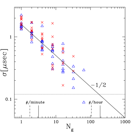
Figure 6: Estimated giant pulse timing precision. At each epoch where 1420 MHz observations were available, the standard deviation $\sigma$ of the giant pulse arrival phase is calculated for MP giants (triangles) and IP giants (X’s), without averaging ($N_{g}=1$). Then consecutive points are pairwise averaged ($N_{g}=2$) and $\sigma$ is calculated again. Pairwise averaging continues as long as the number of points remaining is greater than one. The solid line with slope $-1/2$ is expected for uncorrelated Gaussian timing noise, i.e., $\sigma\propto N_{g}^{-1/2}$. We also plot the number of detectable giant pulses expected in 1-minute and 1-hour intervals for the MP (solid tick) and IP (dashed tick). The dotted line is the timing precision, $\sigma\simeq 120$ ns, achieved with the Mark IV instrument using standard average-profile techniques (Stairs et al. (1999)).

Nevertheless, we have done preliminary estimates of the obtainable timing precision using the current data set. As noted above, a single giant pulse at 1420 MHz can be used to estimate the pulsar phase to $\sim 1.5~{}\mu$s. The key question for timing is whether this precision can be improved by averaging over multiple pulses. If the pulse-to-pulse phase variations are uncorrelated, we expect the timing precision to improve as $\sqrt{N_{g}}$, where $N_{g}$ is the number of consecutive points averaged. In Fig. 6 , we show the r.m.s. scatter $\sigma$ within individual days as a function of $N_{g}$. We find that timing precision improves as expected to the limit of our data sets, $N_{g}=64$, corresponding to a level of 100–300 ns in a ten-minute observation. Also indicated in the figure is the best timing precision achieved using standard pulsar timing techniques, $\sim 120$ ns. Stairs et al. (1999) suggest that the limiting factor in their timing analysis may be pulse shape variations caused by variable interstellar scattering. If this is correct, then giant pulse observations may ultimately improve on normal pulse observations, because the effects of scattering can be much more easily measured and removed from the data. Whether these high-precision timing results on short timescales will lead to better long term timing depends primarily on the long term stability of the giant pulse emission characteristics, which will be studied in future work.

6 Intensity Distribution

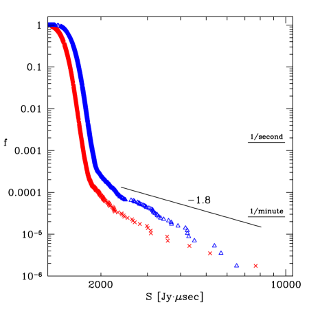
Figure 7: Cumulative intensity distribution for all 150 $\mu$sec windows after the MP (triangles) and IP (X’s) at 430 MHz (15 min.-run on MJD 51364), where $f$ denotes the fraction of pulses containing emission $\geq S$ in the specified windows. Because the giant pulses arrive within the normal emission window, the giant pulses are augmented by the normal emission. This steepens the observed giant pulse power law, leading to a poor fit to the displayed $-1.8$ power law.

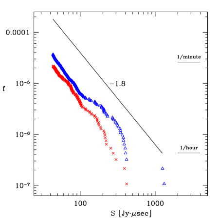
Figure 8: Cumulative intensity distribution for candidate giant pulses at 1420 MHz using the entire 4 hour data set, where $S$ is calculated over 2 $\mu$secs for each candidate and $f$ denotes the fraction of pulses containing candidates arriving in the specified 11.4–$\mu$sec MP (triangles) or IP (X’s) windows with intensity $\geq S$. Also shown is a power law with index $-1.8$.

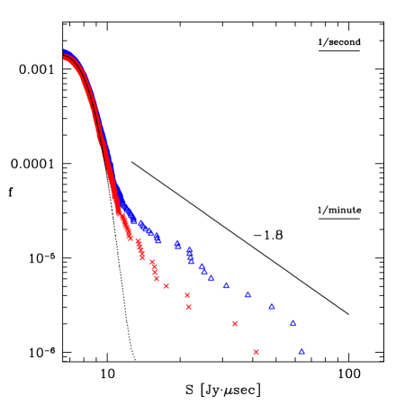
Figure 9: Cumulative intensity distribution for candidate giant pulses at 2380 MHz (26-min. run on MJD 51391), where $S$ is calculated over 2 $\mu$secs and $f$ denotes the fraction of pulses containing candidates arriving in the specified 15.2–$\mu$sec MP (triangles) or IP (X’s) windows with intensity $\geq S$. The dotted line denotes all other candidates from the rest of the pulsar phase scaled to the giant pulse window width of 15.2$~{}\mu$secs. Also shown is a power law with index $-1.8$.

The primary distinguishing characteristic of the giant pulses observed from the Crab Pulsar and PSR B1937$+$21 is, of course, their intensity, and particularly their extended power-law intensity distribution. In Figs. 7–9, we plot the cumulative intensity distribution at each observing frequency. At low intensities, the distributions are dominated by the chi-square statistics of the noise and/or normal emission, but above a certain threshold the pulse strength distribution is roughly power-law distributed. Given our limited statistics for any given run, this simple model is adequate to describe the observed data.

In Fig. 7, we plot the cumulative distribution of the integrated flux densities in $150~{}\mu$sec windows after the MP and IP during a single 15-minute observation at 430 MHz (MJD 51364). Also plotted is the $-1.8$ power-law slope, which Cognard et al. (1996) found for the cumulative giant pulse distribution at this same frequency. The mean signal-to-noise ratio for the normal emission peak in this observation was about $0.14$. Contamination from this emission causes a noticeable deviation at low flux levels from what would be seen with giant pulses and receiver noise alone, causing a steepening of the distribution towards low integrated flux densities. Although the distribution of normal pulse signal strengths is not known, we expect that removing normal pulses would produce better accord with a single power law distribution for the giant pulses. In Fig. 8, we have plotted the cumulative distribution of all giant pulses found at 1420 MHz for all $\sim 4~{}$hours of data (using the threshold detection algorithm described above). Again, generally power-law behavior is observed, with a similar power-law exponent around $-1.8$. In Fig. 9, we plot the cumulative intensity distribution for a $\sim 26$-minute 2380 MHz run (MJD 51391). Again we have plot a $-1.8$ slope for comparison, which appears to fit the MP giant pulses and the most energetic IP giant pulses well, though more data are needed to strengthen this result.

We have also calculated the fraction, $R$, of the total pulsar emission at each frequency that emerges in the form of giant pulses. We find the following ranges at each frequency for this fraction: $0.15\%\leq R\leq 9\%$ (430 MHz), $0.13\%\leq R\leq 4\%$ (1420 MHz), and $0.10\%\leq R\leq 1\%$ (2380 MHz), where the lower limits were determined directly from Figs. 1–3 and the upper limits were determined from Figs. 7–9 by assuming a cumulative distribution with power-law slope of $-1.8$ over all intensities for both the MP and IP giant pulses. From the folded normal emission alone, however, we can rule out large values for $R$ in these calculated ranges, implying that the single power-law model may not be valid at low intensities.

Also consistent with Cognard et al. (1996), we find significantly stronger giant pulses following the MP than the IP. At a given frequency (e.g., 1/minute), the ratio of the strongest giant pulse associated with the MP to the strongest associated with the IP is very roughly the same as the ratio of the peak flux density in the MP to that in the IP. Despite the fact that giant pulses are separated in pulse phase from the normal emission, this suggests a relatively close association between the emission processes.

7 Spectrum

The short timescale of the observed giant pulses imply that they are a relatively broadband phenomenon, with bandwidth greater than their inverse width. The limited bandpass available to the Mark IV instrument prevents stronger statements about the spectra of individual giant pulses. However, the similar arrival distributions and roughly similar arrival rates at each observational frequency point to a broadband phenomenon.

Nevertheless, our observations can be used to constrain the average spectral properties of the giant pulse emission. To avoid complications arising from the use of different effective thresholds at each frequency (because of different source strengths and different receiver noise properties), we estimate the giant pulse spectrum by using the most powerful individual pulses observed during a given time period at each frequency. We have, as usual, calibrated our observations to the spectrum for the average normal emission flux density at each frequency from Foster et al. (1991), as discussed in §2.

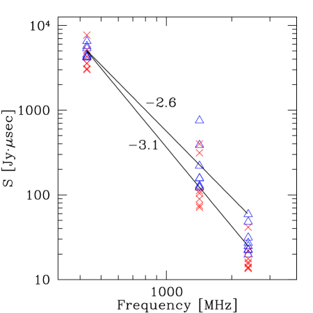
Figure 10: Giant pulse integrated flux density versus frequency for the eight strongest giant pulses in the MP and in the IP taken from equal-length scans of 15 minutes on MJD 51364 (430 MHz), 50893 (1420 MHz), and 51391 (2380 MHz). At each frequency, the absolute flux density calibration was calculated independent of scintillation using the spectral model of Foster et al. (1991). This power-law model has a spectral index for normal emission of $-2.6$; that slope is indicated above. There is some evidence that the spectrum of the strongest giant pulses is steeper; the best fit power-law model, with index $-3.1$, is also shown.

Figure 10 shows the intensities in [Jy$\cdot\mu$sec] of the top eight MP and top eight IP giant pulses at each frequency over 15 minutes, corresponding to the entire MJD 51364 (430 MHz) run and to 15-minute chunks from runs on MJD 50893 (1420 MHz) and MJD 51391 (2380 MHz) We find a somewhat steeper slope of $-3.1$ for the giant pulse spectrum, compared to the $-2.6$ slope for the normal emission spectrum. Although the precise slope of the giant pulse emission spectrum depends on the assumed normal emission spectrum, the result that the giant pulse emission is steeper than the normal emission is robust. However, if the apparent narrowing of the giant pulse emission region at higher frequency reflects a narrowing of a sharp emission cone, the slightly steeper spectrum of the giant pulse emission might be understood as the geometric effect of the position of the line of sight through the outer part of the emission region

Assuming the giant pulses from the Crab pulsar are powered by curvature radiation, Sallmen et al. (1999) have calculated the necessary number and number density of radiating electrons. We perform the same calculation here for our observed giant pulses from PSR B1937$+$21. For coherent curvature radiation, the power emitted by $N$ electrons with relativistic factor $\gamma=(1-v^{2}/c^{2})^{-1/2}$ travelling along magnetic field lines with radius of curvature $\rho_{c}$ is

$$P_{curv}=N^{2}\bigg{(}\frac{2e^{2}\gamma^{4}c}{3\rho_{c}^{2}}\bigg{)}.$$ (1)

From the peak of the largest 1420 MHz giant pulse in Fig. 5, we can calculate the maximum number of electrons needed in one bunch to produce the observed emission (at frequencies greater than 430 MHz). Assuming this pulse is broadband with spectral index, $-3.1$, PSR B1937$+$21 is at a distance of 3.6 kpc, and giant pulse beaming is determined by the beam width $\theta\simeq\gamma^{-1}$, we find a total power at the peak of $\gamma^{-2}\times 10^{34}~{}$erg$\cdot$s^-1. An upper limit on the giant pulse Gaussian FWHM of $\mathrel{\hbox to0.0pt{\lower 3.0pt\hbox{$\mathchar 536\relax$}\hss}\raise 2.0pt\hbox{$\mathchar 316\relax$}}0.5~{}\mu$sec (at high frequencies), gives $\gamma\mathrel{\hbox to0.0pt{\lower 3.0pt\hbox{$\mathchar 536\relax$}\hss}\raise 2.0pt\hbox{$\mathchar 318\relax$}}500$, which implies a substantially smaller power requirement than the total spin-down energy loss rate of $2\times 10^{36}~{}$erg$\cdot$s^-1. Setting $P_{curv}$ equal to the observed power yields

$$N=10^{19}\bigg{(}\frac{\gamma}{500}\bigg{)}^{-3}\bigg{(}\frac{\rho_{c}}{10^{6}~{}\mathrm{cm}}\bigg{)}.$$ (2)

In order to preserve coherence at the highest observational frequency, these electrons must fit within a cube with volume $\mathrel{\hbox to0.0pt{\lower 3.0pt\hbox{$\mathchar 536\relax$}\hss}\raise 2.0pt\hbox{$\mathchar 316\relax$}}\lambda^{3}$, where $\lambda=12.6$ cm at 2380 MHz, implying an electon density of $n_{e}=5\times 10^{15}(\frac{\gamma}{500})^{-3}(\frac{\rho_{c}}{10^{6}~{}\mathrm{cm}})~{}$cm^-3, a value $50$ times greater than the Goldreich-Julian density (Goldreich & Julian (1969)), $n_{{\mathrm{G-J}}}=\Omega B/2\pi e\,c=10^{14}\,(\frac{R}{R_{{\mathrm{NS}}}})^{-3}~{}$cm^-3, which is the electron number density required to power the normal emission via curvature radiation. Sallmen et al. (1999) similarly find a giant pulse electron density $100$ times greater (for $\rho_{c}=10^{7}$ cm) than the Goldreich-Julian value for the Crab pulsar.

8 Discussion

The discovery of giant pulses from a millisecond pulsar was unexpected, and early hopes that identifying commonalities between PSR B1937$+$21 and the Crab pulsar might lead to a better understanding of the giant pulse emission mechanism have so far not been realized. As our study has confirmed, the giant pulse emission from PSR B1937$+$21 differs fundamentally from the Crab giant pulses, despite their common power-law behavior. The most intriguing characteristic of the high-frequency pulses form PSR B1937$+$21 is their very narrow widths and the very limited regions of pulse phase in which they occur.

Despite the continued mystery about their origin, it appears likely that giant pulses from PSR B1937$+$21 may prove a valuable tool. As we have discussed, their narrow intrinsic width and large flux make them attractive fiducial reference points for timing studies of a pulsar that is already among the most precisely timed (Kaspi et al. 1994). Another intriguing possibility is to use the giant pulses as bright flashbulbs to study scattering in the ISM. Because the intrinsic pulses are very narrow, the pulse shape as observed at the Earth traces out the time delays introduced by multipath scattering. The combination of this information with VLBI studies of the scattering disk is a potentially powerful tool for studying the three dimensional distribution of scattering material.

It is important, of course, to identify giant pulse emission from other pulsars. As we have noted, the integrated giant pulse emission from PSR B1937$+$21 is too weak to make noticeable features in the average pulse profiles, so careful, single pulse studies are required. Very fine time resolution is needed to avoid substantially smearing the high-frequency pulses from B1937+21 and reducing their signal-to-noise ratio, and it is insufficient to study only the windows of pulse phase where normal emission is found, as has sometimes been the case in past studies with coherent dedispersion instruments. Instruments that use hardware dedispersion followed by sampling (like the Princeton Mark III, Stinebring et al. (1992)) must also preserve sufficient dynamic range in the analog-to-digital conversion to detect and characterize pulses that are far stronger than the typical pulsar emission. Another subtlety concerning observation of giant pulses are possible projection effects. If the PSR B1937$+$21 giant pulse emission region is roughly Gaussian, then as the pulsar rotates, the giant pulse emission traces out less than $1\%$ of the entire sky, though the likelihood of detecting giant pulses from a known radio pulsar might be substantially enhanced over this estimate by correlations between the angular patterns of the normal and giant emission. Although searches for giant pulse emission from slow pulsars have been unsuccessful, only a very small fraction of millisecond pulsars have been studied sufficiently to detect or rule out giant pulses.

Figure 1: Folded giant pulse emission (solid) and normal emission (dashed) at 2380 MHz (top), 1420 MHz (middle), and 430 MHz (bottom) with unit intensities of 0.07 Jy, $0.24~{}$Jy, and $3.0~{}$Jy (calculated using the power-law model in Foster et al. (1991)) and total integration times at each frequency of 26 minutes, 4 hours, and 30 minutes, respectively. One pulse period equals 4096 bins with each bin $\sim 0.38~{}\mu$secs. The 2380 MHz profile has been rotated so that the MP peak occurs in the same bin as for the 1420 MHz profile. The 430 MHz profiles have been rotated so that the IP peak arrival bin (with scattering taken into account) is coincident with that of the 1420 MHz IP peak. The giant pulse profiles have been amplified by the stated amounts. (Because of differences in receiver noise levels and the giant pulse selection threshold, a comparison of the amplification factors is not physically meaningful.)

Figure 2: Average giant pulse emission (solid) and normal emission (dashed) for the main-pulse region. All other details are the same as for Fig. 1.

Figure 3: Average giant pulse emission (solid) and normal emission (dashed) for the interpulse region. All other details are the same as for Fig. 1.

Freq.	Min.	Normal	Giant	MP delay [$\mu$sec]	IP delay [$\mu$sec]	$\tau$ [$\mu$sec]
2380	25.8	$187.9\pm 0.3^{\circ}$	$189.5\pm 0.5^{\circ}$	$58\pm 1$	$65\pm 2$	$\mathrel{\hbox to0.0pt{\lower 3.0pt\hbox{$\mathchar 536\relax$}\hss}\raise 2.0pt\hbox{$\mathchar 316\relax$}}0.4$
1420	242.6	$187.58\pm 0.01^{\circ}$	$189.5\pm 0.2^{\circ}$	$57\pm 1$	$65\pm 1$	$\mathrel{\hbox to0.0pt{\lower 3.0pt\hbox{$\mathchar 536\relax$}\hss}\raise 2.0pt\hbox{$\mathchar 316\relax$}}1.1$
430	30.0	$\mathrel{\hbox to0.0pt{\lower 3.0pt\hbox{$\mathchar 536\relax$}\hss}\raise 2.0pt\hbox{$\mathchar 318\relax$}}185.6\pm 0.5^{\circ}$	$189.4\pm 0.6^{\circ}$	$\mathrel{\hbox to0.0pt{\lower 3.0pt\hbox{$\mathchar 536\relax$}\hss}\raise 2.0pt\hbox{$\mathchar 318\relax$}}49\pm 2$	$66\pm 2$	$13$–$43$

References

- Backer (1995) Backer, D. C. 1995, J. Astrophys. Astr., 16, 165
- Cognard et al. (1996) Cognard, I., Shrauner, J. A., Taylor, J. H., & Thorsett, S. E. 1996, Astrophys. J., 457, L81
- Foster, Fairhead, & Backer (1991) Foster, R. S., Fairhead, L., & Backer, D. C. 1991, Astrophys. J., 378, 687
- Goldreich & Julian (1969) Goldreich, P. & Julian, W. H. 1969, Astrophys. J., 157, 869
- Hankins & Rickett (1975) Hankins, T. H. & Rickett, B. J. 1975, Meth. Comp. Phys., 14, 55
- Kaspi, Taylor, & Ryba (1994) Kaspi, V. M., Taylor, J. H., & Ryba, M. 1994, Astrophys. J., 428, 713
- Lundgren et al. (1995) Lundgren, S. C., Cordes, J. M., Ulmer, M., Matz, S. M., Lomatch, S., Foster, R. S., & Hankins, T. 1995, Astrophys. J., 453, 433
- Manchester & Taylor (1977) Manchester, R. N. & Taylor, J. H. 1977, Pulsars, (San Francisco: Freeman)
- Sallmen & Backer (1995) Sallmen, S. & Backer, D. C. 1995, in Millisecond Pulsars: A Decade of Surprise, ed. A. S. Fruchter, M. Tavani, & D. C. Backer, Astron. Soc. Pac. Conf. Ser. Vol. 72, 340
- Sallmen et al. (1999) Sallmen, S., Backer, D. C., Hankins, T. H., Moffett, D., & Lundgren, S. 1999, Astrophys. J., 517, 460
- Stairs (1998) Stairs, I. H. 1998. PhD thesis, Princeton University
- Stairs et al. (1999) Stairs, I. H., Splaver, E. M., Thorsett, S. E., Nice, D. J., & Taylor, J. H. 1999, Mon. Not. R. astr. Soc. submitted.
- Stinebring et al. (1992) Stinebring, D. R., Kaspi, V. M., Nice, D. J., Ryba, M. F., Taylor, J. H., Thorsett, S. E., & Hankins, T. H. 1992, Rev. Sci. Instrum., 63, 3551
- Wolszczan, Cordes, & Stinebring (1984) Wolszczan, A., Cordes, J. M., & Stinebring, D. R. 1984, in Millisecond Pulsars, ed. S. P. Reynolds & D. R. Stinebring, (Green Bank: NRAO), 63