The soft X-ray background: evidence for widespread disruption of the gas halos of galaxy groups

Abstract

Almost all of the extragalactic X-ray background (XRB) at 0.25 keV can be accounted for by radio-quiet quasars, allowing us to derive an upper limit of 4 keV cm^-2 s^-1 sr^-1 keV^-1 for the remaining background at 0.25 keV. However, the XRB from the gas halos of groups of galaxies, with gas removal due to cooling accounted for, exceeds this upper limit by an order of magnitude if non-gravitational heating is not included. We calculate this using simulations of halo merger trees and realistic gas density profiles, which we require to reproduce the observed gas fractions and abundances of X-ray clusters. In addition, we find that the entire mass range of groups, from $\sim 5\times 10^{12}$ to $\sim 10^{14}$M_⊙, contributes to the 0.25 keV background in this case.

In a further study, we reduce the luminosities of groups by maximally heating their gas halos while maintaining the same gas fractions. This only reduces the XRB by a factor of 2 or less. We thus argue that most of the gas associated with groups must be outside their virial radii. This conclusion is supported by X-ray studies of individual groups.

The properties of both groups and X-ray clusters can be naturally explained by a model in which the gas is given excess specific energies of $\sim 1$ keV/particle by non-gravitational heating. With this excess energy, the gas is gravitationally unbound from groups, but recollapses with the formation of a cluster of temperature $\mathrel{\hbox to0.0pt{\lower 3.0pt\hbox{$\sim$}\hss}\raise 2.0pt\hbox{$>$}}1$ keV. This is similar to a model proposed by Pen, but is contrary to the evolution of baryons described by Cen & Ostriker.

The excess energy is most likely injected by galaxies in the smaller ‘branches’ of the halo merger tree ($\mathrel{\hbox to0.0pt{\lower 3.0pt\hbox{$\sim$}\hss}\raise 2.0pt\hbox{$<$}}5\times 10^{12}$M_⊙), by active galactic nuclei and possibly supernovae. The heating process may therefore play an important part in the evolution of galaxies.

In addition to the soft XRB spectrum, we simulate source counts in two bands: 0.1–0.4 keV and 0.5–2 keV, for comparison with present and future data.

1 Introduction

Compared to X-ray clusters, relatively little is known about the hot gas halos of galaxy groups (henceforth simply ‘groups’). With the Chandra and XMM satellite missions we can expect much to be revealed about them. However, the extragalactic soft X-ray background (XRB) below $\sim 1$ keV already provides a useful probe of their mean properties. For example, we shall show that (in the absence of non-gravitational heating) the 0.25 keV background probes almost the entire mass range of groups ($\sim 5\times 10^{12}$–$10^{14}$M_⊙, corresponding to temperatures of $T\sim 0.1$–1 keV).

Groups are cosmologically important, for a majority of the baryons in the universe may be associated with them at the present day [Fukugita et al. (1998)]. In addition, groups connect galaxies to clusters in a hierarchical merger tree. This suggests that a large fraction of the heavy elements and ‘excess energy’ (due to non-gravitational heating) injected into the inter-galactic medium (IGM) would have to pass through groups before ending up in X-ray clusters. However, it has been shown that strong heating of the IGM is required to satisfy constraints on the soft XRB [Pen (1999)]. The heating required by Pen, $\delta T\sim 1$ keV, would imply that most of the gas would not be gravitationally bound to the potential wells of groups, contrary to the scenario described above. It is also interesting that this amount of heating is similar to that required to explain the properties of X-ray clusters [Wu et al. (1998), Loewenstein (1999), Pen (1999), Wu et al. (1999)]. Together they therefore suggest a consistent picture of heating in the IGM. Furthermore, the mechanism for heating the IGM is likely to have significant implications for the evolution of galaxies (Wu et al., 1999; hereafter WFN99), whether the heat source be supernovae or active galactic nuclei (AGN).

In this paper, we examine in more detail the contraints on groups, using simulations of halo merger trees and drawing on elements of our semi-analytic model of galaxy formation (WFN99). One important difference from Pen’s model is our inclusion of cooling, in particular its role in removing gas from halos. Our methods for calculating the XRB also differ significantly. Broadly speaking, the main questions we aim to address are whether groups are significantly affected by non-gravitational heating, and if so, what range of groups are affected.

Although a large fraction of the soft XRB below about 0.8 keV originates in our own Galaxy, the extragalactic component can be measured with shadowing experiments. As reviewed by ?), measurements of the extragalactic XRB in the 0.1–0.4 keV band (hereafter 0.25 keV) appear to be converging on a value in the range 20–35 keV cm^-2 s^-1 sr^-1 keV^-1. However, the bulk of the extragalactic XRB is due to AGN. A significant fraction of the XRB at 1 keV has been resolved into AGN. By modelling the QSO X-ray luminosity function and its evolution, ?) estimated the contribution of QSOs to the 1–2 keV XRB (see also [Schmidt et al. (1998)]). Their results correspond to 35–55 per cent of the 1–2 keV background measured by ?). Now, ?) find that radio-quiet quasars have a mean spectral slope of $\alpha=-1.72\pm 0.09$ over the range 0.2–2 keV, though they obtain a significantly flatter slope for (less common) radio-loud quasars. Therefore, if we assume that radio-quiet quasars account for 90 per cent of the quasar contribution to the 1 keV background, then they contribute at least $0.9\times 0.35$ or about 30 per cent of the 1 keV background. Using the 1 keV background measured by ?), which is 9.6 keV cm^-2 s^-1 sr^-1 keV^-1, we can thus obtain a lower limit to the contribution of radio-quiet quasars below 1 keV. At 0.25 keV the lower limit is 31 keV cm^-2 s^-1 sr^-1 keV^-1. From the range quoted by Warwick & Roberts, it follows that gas halos almost certainly contribute less than 4 keV cm^-2 s^-1 sr^-1 keV^-1at 0.25 keV, as most of the 0.25 keV background is already accounted for by QSOs. We shall adopt this value as an upper limit to the contribution from gas halos. (We note that Boyle et al., Laor et al. and the detections quoted by Warwick & Roberts all obtained their data from the same instrument, namely the ROSAT Position Sensitive Proportional Counter.) The main assumption we have made lies in the application of the mean properties measured by Laor et al. to all quasars. On the other hand, we have used the lowest expected contribution of QSOs at 1 keV, along with the highest expected value for the 0.25 keV background. We do not attempt here to assign a confidence level to this limit since the main uncertainties are systematic and not statistical.

The models in this paper are intended to be realistic, but simple enough for comparisons to be easily made. We consider two low-density universes with $\Omega_{m}=0.3$: one with no cosmological constant and the other with $\Omega_{\Lambda}=0.7$. A Hubble constant of $H_{0}=100h$ km s^-1 Mpc^-1 where $h=0.5$ is assumed (the insensitivity of our results to $h$ is discussed in section 3.1). We use CDM-type fluctuation power spectra, normalized to match the observed abundance of X-ray clusters. In this way, the abundance of groups are in effect extrapolated from the X-ray cluster abundance. Likewise, in our fiducial models we assume that groups have a gas fraction of $0.06h^{-3/2}$ when they virialize, as this is the mean value measured for clusters [Evrard (1997), Ettori & Fabian (1999)]. This is a reasonable choice since groups are the progenitors of clusters. Gas halos are assumed to be isothermal and hydrostatically supported in Navarro, Frenk & White (1997; NFW) potential wells. The resulting gas profiles are found to closely model X-ray clusters [Makino et al. (1997), Ettori & Fabian (1999)]. In the absence of excess energy, the model gas profiles of groups and clusters are self-similar to a good approximation. This is a reasonable assumption to make (see hydrodynamic simulations such as Navarro, Frenk & White 1995), especially as we are looking for large differences between model results and observations. We synthesize spectra using the MEKAL spectral synthesis code [Kaastra (1992)].

This paper is organised as follows: in section 2 we describe our model, followed by how we calculate the XRB and source counts. We simulate the XRB from 0.05–2 keV, and calculate source counts in two bands: 0.1–0.4 keV and 0.5–2 keV. In most of sections 2 and 3 we assume that non-gravitational heating is absent. However, we also describe simulations where halos are required to follow observed luminosity-temperature relations extrapolated to lower temperatures. The fiducial results are discussed in section 3. In section 4 we investigate the effects of including non-gravitational heating, and of allowing the gas fraction of halos to be determined by inheritance. We discuss some implications of our results in section 5 and summarize our conclusions in section 6.

2 Simulation

The main components in the calculation of our fiducial results are the halo merger tree, the gas density profiles of virialized halos, and the spectral synthesis model.

The halo merger trees are simulated using the ?) block model, as in our earlier models (e.g. WFN99). The smallest regions simulated have a mass of $1.5\times 10^{10}$M_⊙. We assume a collapse hierarchy of 20 levels, so that the mass of the largest block is $2^{19}\times 1.5\times 10^{10}=7.9\times 10^{15}$M_⊙. This is the total mass of the region simulated in one ‘realisation’ of the merger tree.

The mean density of collapsed halos are specified to conform exactly with the spherical collapse model. In open cosmologies without a cosmological constant, the mean density of a virialized halo is assumed to be $18\pi^{2}\approx 178$ times the background density of an Einstein-de-Sitter universe of the same age. In flat cosmologies with a cosmological constant, we use the analytic approximation given by Kitayama & Suto (1996; equation A6), where the mean density of a halo is given by

$$\rho_{\rm vir}=18\pi^{2}(1+0.4093(\Omega_{m}^{-1}-1)^{0.9052})\overline{\rho}_{b}.$$ (1)

Here, the density parameter, $\Omega_{m}$, and the background density, $\overline{\rho}_{b}$, are evaluated at the time of collapse. At very early times, results from the two prescriptions tend to the same value, as the vacuum density is then small relative to the density of collapsing halos. However, at late times the simple prescription for open cosmologies becomes a poor approximation in $\Lambda$-cosmologies. For example, for a halo that virializes today in a cosmology given by $(\Omega_{m},\Omega_{\Lambda},h)=(0.3,0.7,0.5)$, the first prescription underestimates the mean density by about 20 per cent. Since the X-ray luminosity of a gas halo scales roughly as the density squared, this difference can be significant. From the mass of the collapsed halo, the radius of the halo, $r_{\rm vir}$, thus follows.

The second component in the calculation is the assumed gas density profile of halos. To simplify the synthesis of spectra, we consider only isothermal gas halos. We assume the gas to be in hydrostatic equilibrium in [Navarro et al. (1997)] (1997; NFW) potential wells. In other words, the total density of the halo is described by the NFW profile:

$$\rho(r)={\delta_{c}\rho_{\rm crit}\over(r/r_{s})(1+r/r_{s})^{2}},$$ (2)

where $\rho_{\rm crit}=3H^{2}/8\pi G$ and $H$ is the Hubble parameter at the time of collapse. The parameter $\delta_{c}$ is calculated as described in the Appendix of NFW. The scale radius $r_{s}$ is then uniquely determined by the mean density calculated above. The concentration parameter, $c$, is defined to be $r_{s}/r_{\rm vir}$. (This differs slightly from NFW, as we use a more detailed derivation for the mean density. In particular, their equation (2) that relates $\delta_{c}$ and $c$ is slightly modified in this model.) From the NFW profile, the gravitational potential is given by

$$\phi(x)=\alpha\left(-\frac{\ln(1+x)}{x}+\frac{1}{1+c}\right),$$ (3)

where $x=r/r_{s}$ and $\alpha=4\pi G\rho_{s}r_{s}^{2}$. It then follows that a gas halo of temperature $T$ in hydrostatic equilibrium takes the form

$$\rho_{\rm g}\propto(1+x)^{\eta/x},$$ (4)

where $\rho_{\rm g}$ is the gas density, and $\eta=\mu m_{\rm H}\alpha/(kT)$ (Wu et al., 1998; WFN98). Here, the mean mass per particle of the gas is denoted by $\mu m_{\rm H}$, and $k$ is the Boltzmann constant. This gas profile closely approximates the conventional $\beta$-model if $\beta=\eta/15$ [Makino et al. (1997)], and models most X-ray clusters very well. For large clusters the mean value of $\eta$ is observed to be about 10.5 [Ettori & Fabian (1999)].

We calculate $\eta$ by first specifying the total energy of the gas halo, which then uniquely determines $\eta$. This is described in more detail elsewhere (WFN98; Model B in WFN99). To summarize, in the absence of excess energy, the total specific energy of the gas halo (thermal plus gravitational) is required to be proportional to the specific gravitational energy of the entire halo; we then calibrate this energy relation by matching to the largest clusters. Although halos described by the NFW profile are not exactly self-similar (as the concentration $c$ varies), this relation for the gas halos expresses one form of self-similarity. For the purposes of this paper, the main point to note is that this results in $\eta$ close to 10.5 for all gas halos. In addition, the resulting gas temperatures are well-approximated by $T_{\rm SIS}$, the temperature that the gas would have if both gas and dark matter had power-law density profiles: $\rho\propto r^{-2}$; i.e. $kT_{\rm SIS}/(\mu m_{\rm H})=GM_{\rm tot}/(2r_{\rm vir})$, where $M_{\rm tot}$ is the total mass of the halo. In general, $T$ scatters between $T_{\rm SIS}$ and $1.05T_{\rm SIS}$ for clusters, with the upper end of the range increasing to $1.1T_{\rm SIS}$ as we go down to halo of $\sim 10^{12}$M_⊙.

We assume that isolated galaxies have halo masses of up to $\sim 10^{12}$M_⊙. Since we are primarily concerned with the properties of halos, in this paper the term ‘group’ simply refers to a halo of mass greater than a few $10^{12}$M_⊙ (but less than $\sim 10^{14}$M_⊙).

In our fiducial models, we assume that all halos have a gas mass fraction of 0.17 when they virialize. This is the mean cluster gas fraction measured by ?) and ?) (using $h=0.5$), within a radius $r_{500}$ defined to be such that the mean density within $r_{500}$ is $500\rho_{\rm crit}$. We note that the gas fraction of both observed and simulated clusters tend to increase with the radius within which they are measured. Since $r_{500}<r_{\rm vir}$, it is therefore likely that the true gas fractions of clusters within $r_{\rm vir}$ are higher than this. This strengthens our argument below as it would increase our fiducial estimates of the XRB.

2.1 Calculating the X-ray background

We now describe in detail how we calculate a mean spectrum for the X-ray background. Spectra are simulated using the MEKAL model [Kaastra (1992)], to which we supply two parameters: the gas temperature, $T$, and the metallicity, $Z$, in units of the solar abundance, $Z_{\odot}$ [Anders & Grevesse (1989)]. From the spectrum given by MEKAL, we calculate the cooling function, $\Lambda(T,Z)$. In this way, the model self-consistently estimates the cooling time of the gas.

2.1.1 Cold and hot collapses

We recall that in the collapse of less massive halos, the cooling time of the gas, $t_{\rm cool}$, can be shorter than the free-fall time to the centre of the halo, $t_{\rm ff}$. In this case the gas cools fast enough that it is not hydrostatically supported, and in spite of any shock heating, the gas temperature remains well below the virial temperature most of the time. We refer to this as a cold collapse (WFN99). In our model, gas is labelled as cold when $\tau=t_{\rm cool}/t_{\rm ff}<\tau_{0}$, where $\tau_{0}\sim 1$ is a free parameter. Otherwise, the gas is labelled as hot. This is important when calculating the X-ray background, as we expect cold gas to radiate little, if at all, in the X-ray band. Therefore we only integrate contributions from hot gas and use a fiducial value of $\tau_{0}=1$.

For isothermal gas profiles, $\tau$ is almost always a monotonically increasing function of radius (see Appendix A of WFN99 for a more detailed discussion). This allows us to define a radius, $r_{\rm CF}$, such that gas outside $r_{\rm CF}$ is labelled as hot and gas inside as cold. As halo mass increases, $r_{\rm CF}$ moves from outside the virial radius to the centre of the halo. This transition is fairly abrupt and occurs over about one decade in mass, in halos of $\sim 10^{12}$M_⊙. For halos in the transition region, $r_{\rm CF}$ is found by solving the equation $\tau(r_{\rm CF})=\tau_{0}$ numerically.

(In our model, the transition to the hot-gas regime is made more abrupt by supernova feedback from star formation. We assume that cold gas rapidly forms stars, which lead quickly to type II supernovae. If a sufficient fraction of a collapse is cold, then the energy from supernova feedback is able to eject the rest of the atmosphere, including the hot gas [Nulsen & Fabian (1997)]. By using a much lower value of $\tau_{0}=0.1$, we show that these complications at the transition region have a very small effect on the predicted XRB and source counts, and do not affect our conclusions in any way.)

When a hydrostatically-supported hot gas halo occurs, any gas that cools is assumed to form low-mass stars or ‘baryonic dark matter’, in analogy to cooling flows in X-ray clusters. A possible mechanism for low-mass star formation in cooling flows is described by ?), for the case of elliptical galaxies. It remains possible (if not likely) that some normal star formation and feedback occurs in cooling flows. However this does not affect our main conclusions (the effects of strong heating are investigated in section 4).

2.1.2 Spectral synthesis

We calculate model XRB spectra from $E=0.05$ keV to 2 keV. We first divide this range into equal logarithmic bins of width $\Delta\log_{10}E=0.01$. Suppose photons in the universe belonging to the energy bin $(E,E+\Delta E)$ at the present day have a number density of $\Delta n$, then the corresponding energy flux per steradian (i.e. the intensity) is given by $E\Delta nc/(4\pi)$, where $c$ is the speed of light (in practice, we use the geometric mean of $E$ and $E+\Delta E$ in place of $E$ in this expression). Dividing by $\Delta E$ thus gives the intensity per unit energy, which we express in units of keV cm^-2 s^-1 sr^-1 keV^-1. Below, we refer to these bins as ‘collecting bins’.

Since each realisation of a merger tree simulates a region of constant comoving volume, the photon density $\Delta n$ is simply given by the total number of photons (of the correct energy) emitted in the simulation divided by the present-day volume of the simulation.

We now consider a gas halo at some redshift $z$. Given $T$ and $Z$, its rest-frame spectrum is calculated with MEKAL, also in equal logarithmic bins of width $\Delta\log_{10}E=0.01$. The spectrum is integrated to give the cooling function $\Lambda(T,Z)$—defined such that the bolometric luminosity per unit volume is given by $n_{e}n_{\rm H}\Lambda(T,Z)$, where $n_{e}$ and $n_{\rm H}$ are the electron and hydrogen number densities respectively. We then calculate the number of photons emitted in each ‘rest-frame bin’ per unit total energy that is radiated. These ratios are used throughout the remaining calculation.

For gas radiating at a redshift of $z$, each collecting bin is blueshifted accordingly (from $E$ to $(1+z)E$) to collect photons of the correct energy. Photons from each rest-frame bin are then dumped into the nearest collecting bin. Since the amount of blueshift is a continuous function of $z$, the correspondence between rest-frame bins and collecting bins shifts by one bin each time $(1+z)$ decreases by 0.01 dex. This occurs $\sim 10$ times over the life of a halo (which is the period from one collapse to the next in the block model—we interprete collapses as major mergers).

To summarize, for each halo we calculate the total energy radiated during each time interval between bin shifts. From this the number of photons deposited in each collecting bin is found. The total number of photons collected in the simulation then gives the XRB spectrum as explained above.

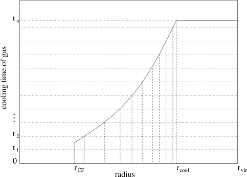
Figure 2: Schematic diagram of how the total energy radiated by a halo is computed. The solid curve encloses the gas emitting in X-rays at any given time: between $r_{\rm CF}$ and $r_{\rm cool}$ it gives the cooling time of the gas, but gas outside $r_{\rm cool}$ does not have time to cool before the next collapse, which occurs at $t_{n}$. Gas inside $r_{\rm CF}$ is labelled as cold and therefore does not contribute to the XRB. The correspondence between rest-frame bins and collecting bins shifts by one position at the times $t_{1},\ldots,t_{n-1}$. Thus the energy radiated during each time interval needs to be calculated. For the gas between $r_{\rm CF}$ and $r_{\rm cool}$, our method involves first dividing the halo into shells, as shown by the dashed lines (see text).

In what follows we describe how we calculate the energy radiated by a halo, taking into account the effects of cooling. The most general case is illustrated in Fig. 2, which shows the amount of gas contributing to the XRB as a function of time. Also shown are the times $t_{i}$ ($i=1,2,\ldots,n-1$) when bin shifts occur, measured from when the halo virializes. $t_{n}$ gives the time of the next collapse.

Gas inside $r_{\rm CF}$ is regarded as cold and therefore is not included in the calculation. Between $r_{\rm CF}$ and the cooling radius, $r_{\rm cool}$, the cooling time is shorter than the time to the next collapse: gas in this region is assumed to cool out once its cooling time has elapsed. The cooling time is estimated by

$$t_{\rm cool}={3\over 2}{\rho_{\rm g}kT/\mu m_{\rm H}\over n_{e}n_{\rm H}\Lambda(T,Z)}.$$ (5)

As explained in WFN99, the gas profile that we use to estimate such quantities must be regarded as notional, as it cannot describe the gas halo at all times. In particular, the gas halo redistributes itself as gas in the centre cools out. Nevertheless, the gas profile allows us to estimate the behaviour of different subsets of gas in the halo.

Between $r_{\rm cool}$ and $r_{\rm vir}$, gas does not have time to cool before the next collapse. Here, the energy radiated during each time interval is easily calculated from its bolometric luminosity, which is given by $\int_{r_{\rm cool}}^{r_{\rm vir}}n_{e}n_{\rm H}\Lambda(T,Z){\rm d}V$. The number of photons dumped into each collecting bin thus follows.

This is less straightforward to apply to the gas inside $r_{\rm cool}$, because the amount of gas changes continuously with time. However, the gas inside $r_{\rm cool}$ cools completely, so that the energy radiated is simply given by $(3/2)NkT$, where $N=\int\rho_{\rm g}/(\mu m_{\rm H}){\rm d}V$ is the number of particles that cool. To estimate the amount of energy radiated in each time interval, we first divide the halo into shells separated by the radii $R_{\rm cool}(t_{i})$. The function $R_{\rm cool}(t)$ gives the radius where cooling time is equal to $t$. For the shell with an outer radius of $R_{\rm cool}(t_{i})$, we assume that $(t_{j}-t_{j-1})/t_{i}$ of the energy it radiates (as given above) is emitted in the $j$-th time interval. In this way, the total energy radiated is correctly accounted for, but the ‘allocation’ of energies between time intervals is less precise. However, the latter is equivalent to determining how the photons are binned, and the binning of photons is already uncertain by $\pm 1$ bin, because the bin shifts are uncontinuous. It follows that the derived spectrum is ‘smeared’ by $\sim 1$ bin width.

Note that the release of $(3/2)kT$ per particle that cools must be regarded as a lower limit: in reality, the weight of the overlying gas is likely to at least maintain the pressure of the gas as it cools, so that gravitational work raises the total energy radiated to $(5/2)kT$ per particle or more in most cases. In addition, the density of the gas increases as it cools and moves to smaller radii, so that the luminosity of a given parcel of gas increases. As a result, $(3/2)kT$ leads to a reasonable estimate of the cooling time. For the gas outside $r_{\rm cool}$, the density also increases as the gas moves inwards. Therefore, our estimate of the energy released in this case should also be a lower limit.

A caveat of our model is that any intrinsic absorption that might occur in the cooling region (in analogy to cluster cooling flows) is ignored. Since this is confined to the cooling region at any given time, while most of the simulated XRB arises from outside that region, its effect is unlikely to be important.

2.2 Source counts

The $\log N$–$\log S$ function for X-ray halos is calculated in two bands: the 0.1–0.4 keV band, for comparison with future results from Chandra and XMM, and the 0.5–2 keV band, for comparison with results from the Wide-Angle ROSAT Pointed X-ray Survey (WARPS; Scharf et al. 1997) and the slightly deeper counts made by ?).

Since the simulated merger trees provide no spatial information, it is assumed that the halos are distributed randomly in space. The probability of a given source in the simulation being observable in principle (with an infinitely sensitive telescope) depends on how long it ‘exists’. Suppose a source exists for a short period corresponding to ${\rm d}z$. The comoving volume observable by us on the entire sky in this redshift interval is given by

$${\rm d}V_{c}={c\over H_{0}}{[D_{L}(z)/(1+z)]^{2}\over\sqrt{\Omega_{m}(1+z)^{3}+(1-\Omega_{m}-\Omega_{\Lambda})(1+z)^{2}+\Omega_{\Lambda}}}4\pi|{\rm d}z|,$$ (6)

where $D_{L}(z)$ is the luminosity distance (given below). Suppose we create an infinite universe by tiling together copies of the same simulation. Then the mean number of copies of this particular source that we expect to see is given by ${\rm d}V_{c}$ divided by the volume of simulation. This is therefore the contribution of this source to the mean source count on the whole sky.

We integrate source counts for fluxes of $S=10^{-16}$–$10^{-13}$ erg s^-1 cm^-2, which we divide into logarithmic bins of width $\Delta\log_{10}S=0.1$. The flux from a gas halo is given by $S=L_{\rm X}/(4\pi D_{L}^{2})$, where $L_{\rm X}$ is the luminosity in the relevant, blueshifted band. For $\Omega_{\Lambda}=0$, $D_{L}$ is given by (e.g. Peacock 1999):

$$D_{L}=(1+z){2c\over H_{0}}{\Omega_{m}z+(\Omega_{m}-2)(\sqrt{1+\Omega_{m}z}-1)\over\Omega_{m}^{2}(1+z)},$$ (7)

but for $\Omega_{m}+\Omega_{\Lambda}=1$, $D_{L}$ is integrated numerically:

$$D_{L}=(1+z){c\over H_{0}}\int_{0}^{z}{{\rm d}z^{\prime}\over\sqrt{\Omega_{m}(1+z)^{3}+\Omega_{\Lambda}}}.$$ (8)

Equation 6 is integrated over the lifetime of a given halo in the simulation, to give the mean number of copies of that halo that we expect to see on the sky. To do this we associate $\Delta z$ with the same time intervals described in the previous section. This gives a good approximation for the cosmologies and redshifts that we are interested in. Luminosities and fluxes are calculated at the beginning of each time interval. Each interval then contributes to the number count in the relevant flux bin as described above. (Using the average luminosity in each time interval only changes the number counts by $\sim 5$ per cent.)

We tested our code by summing all the discrete sources to give an alternative calculation of the XRB at a given energy. To do this we replaced the above energy bands with one very narrow band at this energy, and integrated the total flux in this band. The resulting intensity per keV agreed well with the spectrum derived using our usual method.

2.3 Empirical calculations based on $L_{\rm X}-T$ relations

It is well-known that self-similar gas halos (such as those described at the beginning of this section) do not match the observed properties of X-ray clusters. Substantial heating is required to lower the luminosities of the smaller clusters, in order to match the observed relation of $L_{\rm X}\propto T^{3}$ (WFN98,99; Pen 99). How this extends to groups is less clear. A clue is offered by the $L_{\rm X}-T$ distribution of the Hickson Compact Groups or HCGs [Ponman et al. (1996)], which is significantly steeper than that for clusters. However, this only extends down to about 0.5 keV, and the scatter in the distribution appears to be intrinsically very large. (In section 4, we propose a reason for the large scatter.) The steeper $L_{\rm X}-T$ relation for groups suggests that the effects of heating are even more severe than in clusters. Other X-ray studies of groups [Mulchaey et al. (1996), Helsdon & Ponman (1999)] confirm this view.

Since we only require the temperature and bolometric luminosity of a gas halo in order to estimate its spectrum, we have performed separate simulations based on (extrapolations of) observed $L_{\rm X}-T$ relations. A basic difficulty with the $L_{\rm X}-T$ relation for groups is that a large fraction of groups do not have detectable X-ray emission, so that an X-ray selected sample is likely to give a biased estimate of the average luminosity. In fact, optically-selected samples also face difficulties, as they may include chance projections of galaxies. On top of this, the X-ray temperature of a group can differ significantly from the temperature associated with the velocity dispersion $\sigma$ of the galaxies [Ponman et al. (1996), Helsdon & Ponman (1999)]. If we suppose that $\sigma$ reflects the underlying dark matter distribution, then the gas temperature in the self-similar case is approximately given by $kT/(\mu m_{\rm H})=\sigma^{2}$. In reality, the $T-\sigma$ distribution for groups exhibits a large scatter about the best-fit power law, which has a different slope from the self-similar relation. For the HCGs, the best-fit power law yields temperatures (as a function of $\sigma$) than are up to a factor of 2 higher than the self-similar prediction [Ponman et al. (1996)].

Faced with these uncertainties, we have simply applied the observed $L_{\rm X}-T$ relations and assumed that $T$ is the same as the temperature given in the self-similar model. In addition, we assume that the luminosity of a halo remains constant during its lifetime. This is reasonable because the time-averaged luminosity of a halo in the simulation should correspond to the observed luminosities averaged over many groups. In this way, we are able to calculate XRB spectra and source counts as described above. Although crude, the results give an insight into what the true composition of the soft XRB might look like.

The best-fit $L_{\rm X}-T$ relation for the HCGs is given by [Ponman et al. (1996)]:

$$\log L_{\rm bol}=(43.17\pm 0.26)+(8.2\pm 2.7)\log T,$$ (9)

where $L_{\rm bol}$ is the bolometric luminosity in erg s^-1 and $T$ is in keV. As noted above, we also apply this relation below its observed range. Despite the uncertainty in the slope, it is clearly much steeper than the relation for clusters. For clusters, we use the best-fit given by ?):

$$\log L_{\rm bol}=(42.7\pm 0.1)+(2.98\pm 0.11)\log T.$$ (10)

This spans a range of $T\approx 2$–10 keV. The two relations intersect at $T=0.8$ keV. Thus we are able to apply the cluster relation above 0.8 keV, and the group relation for lower temperatures. We refer to this combination as ‘PW’. We also perform simulations with only the cluster relation, extrapolated to all temperatures. We refer to these as ‘W’ simulations.

In the simulations, we do not include scatter in the above relations. This is permissible for estimating the XRB, which depends on the mean properties of halos. However scatter can significantly affect the resulting source counts. For our purposes, this is more easily adjusted for after the simulation, and we discuss it with the results.

3 Fiducial results

3.1 Calibration

Perhaps the two most important ‘parameters’ in this study are the gas fraction and the mass function of the relevant halos.

For the fiducial models discussed in this section, we set the initial gas fraction of all halos to be 0.17. Although this may be unrealistic in detail, it provides a simple point of reference. As for the mass function of groups, the primary constraint, albeit indirect, is the mass function of X-ray clusters at $z=0$. We require all of our simulations to reproduce the temperature function of X-ray clusters, for which we use the best-fit power law measured by ?). (The temperature function is a reasonably direct way of constraining the mass function of clusters, whereas the luminosity function is sensitive to other properties, such as the gas fraction and the structure of gas halos.) It follows that the abundance of less massive halos are in effect extrapolated from the observed cluster abundance, by assuming CDM power spectra. To investigate the inherent uncertainty in this, we consider two different values for the CDM shape parameter $\Gamma$.

As in WFN99, we assume a baryon density parameter of $\Omega_{b}=0.02h^{-2}=0.08$ [Burles & Tytler (1998), Burles et al. (1999)]. Following ?), the CDM shape parameter is then given by $\Gamma=\Omega_{m}h\exp(-\Omega_{b}(1+\sqrt{2h}/\Omega_{m}))=0.106$. Using this value of $\Gamma$ in an OCDM universe with $(\Omega_{m},\Omega_{\Lambda},h)=(0.3,0,0.5)$, we are able to match the temperature function of X-ray clusters using $\sigma_{8}=0.75$ (as shown in WFN99).

For a $\Lambda$CDM cosmology with $(\Omega_{m},\Omega_{\Lambda},h)=(0.3,0.7,0.5)$ and the same values for $\Omega_{b}$ and $\Gamma$, we are able to reproduce the cluster temperature function using $\sigma_{8}=0.8$. Both of the above results for $\sigma_{8}$ agree remarkably well with Eke et al. (1998, and private communication for $\Lambda$CDM).

For each cosmology, we also consider a higher value of $\Gamma=0.25$, as measured by ?) from galaxy surveys. In both cosmologies, we find that the same values of $\sigma_{8}$ are able to reproduce the cluster temperature function, in agreement with Eke et al. (1998).

Table 2: List of simulations and legend for Figs. 4–6 and Figs. 16–22. Each line in the table corresponds to two simulations, performed in the OCDM and $\Lambda$CDM cosmologies. Only the parameters that change between simulations have been listed. The ‘W’ and ‘PW’ simulations are described in section 2.3.

line-style	metallicity ($Z_{\odot}$)	$\tau_{0}$	$\Gamma$	$L_{\rm X}-T$ fixed?
solid	0.3	1	0.106	no
dotted	0.03	1	0.106	no
dashed	0.3	1	0.25	no
dot dash	0.3	0.1	0.106	no
dash dot dot dot	0.3	1	0.106	yes, W
long dashes	0.3	1	0.106	yes, PW

A list of simulations is given in Table 2, which we repeat for each cosmology. The table gives the values of parameters that vary between simulations. We assume the same metallicity for all gas halos in any given simulation. For each simulation that assumes no non-gravitational heating (‘no’ in the last column), we use 100 realisations of the merger tree. These simulations produce similar results to each other. Thus, to test that their results have converged, we increased the number of realisations in one of these simulations by a factor of 4. This made no noticable difference to the results.

In the simulations based on extrapolations of observed $L_{\rm X}-T$ relations (‘yes’ in the last column), the XRB is dominated by more massive halos, so that 400 realisations are required to obtain convergence.

Finally, we note that our results are not sensitive to increases in $h$. For our fiducial simulations that assume self-similarity, this can be understood by noting that the model is normalized to reproduce the contribution of the largest observed clusters (which are close to self-similar, [Allen & Fabian (1998)]) to the XRB. Since that contribution is a directly measured quantity, it has no dependence on $h$. The rest of the simulated XRB is then a non-trivial extrapolation of the cluster contribution. A similar argument applies to all our simulations.

To test the sensitivity, we also simulated the first model in Table 2 using $h=0.7$, without changing $\Gamma$ and using $\Lambda$CDM. The gas fraction of clusters scales as $h^{-3/2}$, but this is compensated by the number density of halos—as expressed by the temperature function—which scales approximately as $h^{3}$. The resulting XRB spectrum is about 10 per cent higher and the source counts (in the given flux range) are virtually unchanged.

3.2 The XRB spectrum from hot gas halos

Figure 4: Simulated XRB spectra in the OCDM cosmology. The legend for the different lines is given in Table 2. The upper limit for the gas halo contribution to the observed 0.25 keV background is shown by the arrow.

Figure 6: As Fig. 4, but in the $\Lambda$CDM cosmology.

The XRB spectra from the simulations listed in Table 2 are displayed in Figs. 4 and 6, for OCDM and $\Lambda$CDM respectively. It is clear from the two figures that the two cosmologies produce similar results. (The OCDM spectra are only slightly higher than the $\Lambda$CDM spectra, by up to a factor of 1/3 depending on the energy.) The 0.25 keV backgrounds predicted by the simulations that assume no heating are all much higher than our upper limit of 4 keV cm^-2 s^-1 sr^-1 keV^-1 (section 1)—several by over an order of magnitude. These simulations also overpredict the 1 keV background, which should be about 1 keV cm^-2 s^-1 sr^-1 keV^-1; the extragalactic background at 1 keV is about 10 keV cm^-2 s^-1 sr^-1 keV^-1 [Gendreau et al. (1995)], but only about 10 per cent of this is likely to be from groups and clusters [McHardy et al. (1998)].

To illustrate the importance of cooling, we modified one of these simulations as follows to switch off cooling. For all halos that contribute to the XRB in the fiducial simulation, a) we label all of their gas as hot (thus $r_{\rm CF}=0$), and b) we suppose that no gas is removed as a result of cooling. This increases the 0.25 keV background by a factor of 5, and increases the 1 keV background by almost 3-fold. These large increases show that if cooling is not included, then gas will often end up radiating many times its thermal energy. (In this case, our results increase to a level comparable to the 0.25 keV background calculated by Pen (1999), using clumping factors obtained from hydrodynamic simulations.)

We shall now discuss the differences between the above spectra. We regarded the parameters used to obtain the solid spectra as the ‘default’ parameters (Table 2) and varied each of the parameters in turn to observe the consequences. Reducing the metallicity from 0.3 to 0.03 $Z_{\odot}$ (dotted spectra) reduced the amount of line-emission, so that the resulting XRB spectrum is much smoother. By comparison, a large ‘bump’ in the solid spectrum at around 0.7 keV can be seen. It corresponds to the (redshifted) iron L complex. However, the changes at the other energies are more modest; the spectrum is almost independent of metallicity at 0.25 keV. It is interesting that the XRB spectrum increases at certain energies when we reduce the metallicity. This occurs in parts of the spectrum where line-emission is weak. It is possible because the cooling time of gas increases when we reduce the metallicity. Increasing the CDM shape parameter to $\Gamma=0.25$ (dashed spectra) raises the power at sub-cluster scales, resulting in more galaxy groups. In both cosmologies, this raises the XRB spectrum by roughly 50 per cent.

Figure 8: Plot of halo contributions to the XRB at 0.25 keV, for the case of the solid spectrum in the $\Lambda$CDM cosmology (Fig. 6). The solid lines correspond to the left axis, and the dotted line to the right axis. The squares give the fractional contribution from all halos of a given mass, and the triangles give the mean contribution from those halos. The squares in effect give the contribution per unit logarithmic interval in mass. The crosses show the number of hot gas halos obtained in the simulation; thus the squares are the product of the triangles and crosses.

Figure 10: As Fig. 8, but for the XRB at 1 keV.

To better understand the implications of these results, we need to know which types of halo are contributing to the soft XRB. We therefore computed the fractional contribution of halos belonging to each mass in the block model. This was done at two energies: 0.25 keV and 1 keV, which correspond to the two energy bands used in our source counts. In Figs. 8 and 10 we show the fractional contributions to the solid spectrum in the $\Lambda$CDM case (Fig. 6), at 0.25 keV and 1 keV respectively. The corresponding plots for the OCDM case are almost the same, and the results for the dotted and the dashed spectra are very similar. In these plots, the solid lines correspond to the axis on the left and the dotted line to the axis on the right. The main result is given by the squares, which show the fraction of the XRB due to all halos of a given mass (since the masses increase by factors of 2, this is equivalent to the contribution per unit logarithmic interval in mass).

At 0.25 keV (Fig. 8), the squares form a relatively flat plateau from $\sim 5\times 10^{12}$M_⊙ to $\sim 10^{14}$M_⊙. In other words, the 0.25 keV background is contributed by almost the entire range of halos corresponding to groups. We assume that isolated galaxies have total masses of up to $\sim 10^{12}$M_⊙, and that an X-ray cluster with a temperature of 1 keV has a mass of $\sim 10^{14}$M_⊙. This result means that if we wish to match our upper limit on the 0.25 keV background, then we must reduce the contributions of almost all groups.

The triangles in Fig. 8 give the mean fractional contribution per halo as a function of mass. The plus signs give the total number of hot gas halos obtained in the simulation. Therefore, the product of these two curves reproduce the flat plateau traced by the squares.

The situation is quite different for the XRB at 1 keV. In Fig. 10 the squares peak quite sharply at around $6\times 10^{13}$M_⊙. The difference is brought about by the much steeper curve traced by the triangles, because less massive halos contribute less at 1 keV.

Figure 12: As Fig. 8, but for the dot-dashed spectrum at 0.25 keV in the $\Lambda$CDM cosmology. Lowering $\tau_{0}$ to 0.1 results in hot gas halos at lower masses. In addition, the low-mass drop-off in the squares is now due to the sharp decline in contribution per halo (shown by the triangles), which should be contrasted with Fig. 8.

Returning to Fig. 8, we note that the sharp drop in contributions below $4\times 10^{12}$M_⊙ appears to be entirely due to the low-mass ‘cutoff’ in the dotted curve (cf. Fig. 10). This ‘cutoff’ results from the transition from cold to hot collapses, which is controlled by the parameter $\tau_{0}$. Therefore, to investigate the sensitivity of the XRB to $\tau_{0}$, we reduced its value from 1 to 0.1. This gave the dot-dashed spectra in Figs. 4 and 6, which show only a small increases from the solid spectra (about 25 per cent at 0.25 keV). For the $\Lambda$CDM case, we show the new breakdown of contributions at 0.25 keV in Fig. 12. The curves now extend to a lower mass, showing that the plateau does indeed end around $4\times 10^{12}$M_⊙, even though the transition from cold to hot collapses has been pushed to less massive halos. This explains why the 0.25 keV background is not sensitive to the parameter $\tau_{0}$.

Figure 14: As Fig. 8, but for the ‘W’ simulation in the $\Lambda$CDM case. The plot shows halo contributions to the 0.25 keV background when the luminosities of groups are reduced to match the extrapolated $L_{\rm X}-T$ relation from White et al. (1997). By doing so, the background gradually becomes dominated by halos at $\sim 10^{14}$M_⊙. In the ‘PW’ simulation the luminosities of most groups are reduced much further, but the 0.25 keV background does not drop much as it becomes ‘supported’ by halos of order $10^{14}$M_⊙.

For the last two simulations listed in Table 2, we fixed the luminosities of halos according to observed $L_{\rm X}-T$ relations, as described in section 2.3. The resulting spectra, shown in Figs. 4 and 6, satisfy our upper limit on the 0.25 keV background. In addition, the 1 keV background in the OCDM case is very close to 1 keV cm^-2 s^-1 sr^-1 keV^-1, as expected from observations (see above). (In the $\Lambda$CDM case, the 1 keV background is slightly smaller.) In spite of the great difference in the $L_{\rm X}-T$ slopes adopted for groups, the ‘W’ and ‘PW’ simulations produce spectra that differ by less than a factor of 1/3. The reason for this is illustrated in Fig. 14 and discussed in the caption. Notice that even in the ‘W’ case, the contributions of individual groups at 0.25 keV have been reduced by an order of magnitude or more, across the entire mass range. In a further simulation, we took the $L_{\rm X}-T$ relation from the ‘PW’ simulation and ‘pivoted’ the slope below the intersection point at 0.8 keV, to give $L_{\rm X}\propto T^{2}$ (so that luminosities are higher than in the ‘W’ simulation). This increased the spectrum around 0.25 keV by a factor of 1/3 relative to the ‘W’ simulation.

3.3 Source counts

Figure 16: Simulated $\log N$–$\log S$ functions in the 0.1–0.4 keV band, for the OCDM cosmology. The legend for the different lines is given in Table 2.

Figure 18: As Fig. 16, but showing source counts in the 0.5–2 keV band (OCDM cosmology). The heavy dotted-line approximates the observed source counts.

Figure 20: Simulated $\log N$–$\log S$ functions in the 0.1–0.4 keV band, for the $\Lambda$CDM cosmology. The legend for the different lines is given Table 2.

Figure 22: As Fig. 20, but showing source counts in the 0.5–2 keV band ($\Lambda$CDM cosmology). The heavy dotted-line approximates the observed source counts.

The source counts from the above simulations are displayed in Figs. 16 to 22. Figs. 16 and 18 show results from the OCDM simulations in the 0.1–0.4 keV and 0.5-2 keV bands, respectively. Likewise, results for $\Lambda$CDM are shown in Figs. 20 and 22.

As with the spectra, the $\log N$–$\log S$ curves fall clearly into two groups in each figure, given by the first four and the last two simulations listed in Table 2. Little data exists for comparison, except above $10^{-14}$ erg s^-1 cm^-2 in the harder band. The $\log N$–$\log S$ function from the WARPS survey [Jones et al. (1998)] extends down to $6\times 10^{-14}$ erg s^-1 cm^-2, and the $\log N$–$\log S$ function of ?) covers fainter fluxes down to $1\times 10^{-14}$ erg s^-1 cm^-2. Both observed functions are closely approximated by the simple equation $N(>S)=(10^{-13}\mbox{erg~{}s${}^{-1}$~{}cm${}^{-2}$}/S)$, which lies an order of magnitude below the ‘self-similar’ predictions shown in Figs. 18 and 22. This is to be expected, for the sources in this flux range are identified as small clusters in the simulation, with temperatures of $\sim 1$ keV. Hence, we already know that they should not be self-similar, as they lie at (or just off) the lower end of the $L_{\rm X}-T$ relation of ?).

Several of the differences between the $\log N$–$\log S$ functions can be traced back to the spectra. For example, the dotted and solid curves (which differ in the metallicity used) are very close in the 0.1–0.4 keV band, but differ by almost a factor of 2 in the 0.5–2 keV band. As discussed above, this can be attributed to the iron L complex. Reducing $\tau_{0}$ to 0.1 (dot-dashed curves) increases the number of low-mass halos with hot gas; this makes negligible difference in the 0.5–2 keV band, but some change can be seen in the 0.1–0.4 keV band. In all cases, increasing the CDM shape parameter to $\Gamma=0.25$ increases the number counts by roughly 50 per cent, though this depends somewhat on the flux.

The $\log N$–$\log S$ functions from the ‘W’ and ‘PW’ simulations differ little from each other, especially above $10^{-14}$ erg s^-1 cm^-2. This is because the counts are mostly dominated by (small) clusters in both cases. Therefore they do not depend on which $L_{\rm X}-T$ relation we use for groups. This suggests that the predictions in the 0.5–2 keV band above $10^{-14}$ erg s^-1 cm^-2 should come close to the observed counts, since we have imposed the observed $L_{\rm X}-T$ relation for clusters and fitted the observed cluster temperature function. However, the model source counts are a factor of 2 to 3 smaller. The main reason for this discrepancy is because we do not include any scatter in the $L_{\rm X}-T$ relation used in the simulations. The XRB is not sensitive to scatter, for it measures the mean properties of halos. However, scatter in the flux of sources, when combined with the large number of faint sources compared to bright ones, can significantly increase the model $\log N$–$\log S$ function.

We now describe a simple correction for this effect. We first note that the best-fit $L_{\rm X}-T$ relation of ?) is calculated in logarithmic space. Therefore the simplest way to include scatter is to give $\log L_{\rm X}$ (at each temperature) a gaussian distribution centred on the value given by the best-fit. Let the standard deviation, $\sigma$, be independent of temperature (see their Fig. 1a). It follows that the new ${\rm d}N/{\rm d}S$ distribution is given by convolving the old one with this gaussian, with $\log S$ as the independent variable. We now approximate the model $\log N$–$\log S$ functions (for $S>10^{-14}$ erg s^-1 cm^-2) by the power law $N(>S)\propto 1/S$—as we did for the observed source counts—which implies ${\rm d}N/{\rm d}S\propto 1/S^{2}$. It is not hard to show that ${\rm d}N/{\rm d}S$ remains a power law when convolved with the gaussian, but it is shifted upwards by a factor of $10^{2\sigma^{2}\ln 10}$. Therefore an intrinsic scatter in $\log L_{\rm X}$ of $\sigma=0.3$ (i.e. a factor of 2 in each direction) increases $N(>S)$ by a factor of 2.6. This brings the model $\log N$–$\log S$ functions roughly in agreement with the data. However, the true intrinsic scatter for small clusters is not well determined, and this result highlights the inherent uncertainty in modelling source counts. This correction should also be applied to the 0.1–0.4 keV band where the slope of $N(>S)$ is the same. At much lower fluxes, a sizable contribution from groups is not ruled out (see Figs. 16 to 22). If their scatter is very large (as discussed below), then their counts would be increased in the same way.

4 Further investigations

4.1 Non-gravitational heating while maintaining the same gas fractions

Here we discuss an example of heating that fails remarkably to reduce the simulated XRB to the required level.

In our heating models described in WFN99, we allow the total energy of gas halos (the sum of thermal and potential energies) to increase in the presence of excess energy from non-gravitational heating. This both raises the gas temperature and flattens the density profile of a gas halo, but we maintain the same gas mass within $r_{\rm vir}$. For the isothermal gas profiles used in this paper, this is modelled by reducing the slope parameter $\eta$. The X-ray luminosity can be reduced by up to an order of magnitude as a result, before the total energy of the gas halo becomes positive (relative to the appropriate potential), at which point we regard the gas as gravitationally unbound.

Figure 24: Further simulated spectra in the OCDM cosmology. The solid spectrum from Fig. 4 is shown here for comparison. The dashed spectrum was obtained by heating all gas halos to the point of being marginally bound (see section 4.1). For the dotted spectrum, the gas fractions of halos were determined naturally from their progenitors (section 4.2). The dot-dashed spectrum was given by a preliminary study of the injection of excess energy by galaxies, which simultaneously fits the $L_{\rm X}-T$ relations for clusters (section 4.3).

Figure 26: As Fig. 24, but for $\Lambda$CDM. (The solid spectrum is taken from Fig. 6.)

In two further simulations, we modify the first model in Table 2 by heating the gas in all halos $>3\times 10^{12}$M_⊙ to the point of being marginally bound, whilst retaining a gas fraction of 0.17. (100 realisations were used in these simulations.) The strong heating roughly doubles the temperature of a halo and halves the value of $\eta$. These simulations may be expected to give the maximum possible reduction in the XRB given a gas fraction of 0.17. However, the resulting XRB spectra, given by the dashed curves in Figs. 24 and 26, show a reduction of only a half (at 0.25 keV) compared to the solid spectrum.

Figure 28: Plot of halo contributions to the 0.25 keV background when gas halos are maximally heated as described in section 4.1, for the $\Lambda$CDM case. The symbols are described in Fig. 8.

Notice that we have not heated halos below $3\times 10^{12}$M_⊙. Doing this doubles the dashed spectrum at 0.25 keV, due to a whole new contribution from halos of $\sim 10^{12}$M_⊙—based on the criterion of $\tau_{0}=1$, these halos become hot collapses (see section 2.1.1) as a result of their increased cooling times. However, we are more interested in how much we can reduce the XRB.

Fig. 28 shows the new distribution of halo contributions for $\Lambda$CDM. Except for the point at $4\times 10^{12}$M_⊙, the total contributions (squares) at all higher masses are reduced by the heating. (The contribution at $4\times 10^{12}$M_⊙ increases for the same reasons given above, but the effect on the total 0.25 keV background is small.) The reason for the rather modest reduction in the 0.25 keV background has to do with the large fraction of gas able to cool in the smaller groups when heating is absent. The fraction of gas that is able to cool decreases gradually as we progress to massive groups. The depletion of gas from the centres of halos can greatly reduce the luminosity, so that even when heating is absent the groups do not follow $L_{\rm X}\propto T^{2}$ on average, but obey a steeper relation. When the halos are heated in the manner described, the fraction of gas able to cool becomes small even in small groups, and we recover $L_{\rm X}\propto T^{2}$ (because $\eta\approx 5$ in all groups) normalized to a lower luminosity. Thus, the modest reduction of the XRB may be attributed to the already-reduced luminosities of groups (averaged over time) due to cooling. This also explains why heating reduces the contributions of large groups more than for small groups, as shown by the sloping curve in Fig. 28 (cf. Fig. 8).

Note that if we impose $L_{\rm X}\propto T^{2}$ for all groups and clusters when heating is absent, then this corresponds to ignoring the effect of cooling. As we mentioned in the previous section, this results in a 0.25 keV background that is 5 times higher than our fiducial result, and therefore about 10 times higher than the dashed spectra.

The inability of this method to reduce the 0.25 keV background to a level that is even close to the upper limit, implies that the gas fractions of groups (before the gas cools) must be much lower than 0.17. In principle, we can remove, say, all of the gas in groups below $2\times 10^{13}$M_⊙ (see Fig. 28), which would bring the 0.25 keV background just below the upper limit; but the model is already so contrived that groups are almost certainly gas-poor up to $\sim 10^{14}$M_⊙. This conclusion is supported by results from X-ray studies of individual groups. Since the average gas fraction of clusters is at least 0.17, we argue that a large fraction of the gas belonging to groups must be outside their virial radii (see below).

4.2 Gas fractions determined by inheritance

So far, we have fixed the initial gas fractions of groups at 0.17. We now consider the effect of relaxing this assumption, so that the amount of gas in a halo is naturally determined by the amount accreted or inherited from its progenitors. We use the same parameters as the first model in Table 2, but modify the primordial gas fraction so that we obtain large clusters with gas fractions close to 0.17. In the OCDM case, we use a primordial gas fraction of 0.25, and for $\Lambda$CDM we use 0.23. ($\Gamma$ is increased marginally by the new values of $\Omega_{b}$, according to [Sugiyama (1995)].) As in the fiducial simulations, we assume no non-gravitational heating. 100 realisations were used in each simulation. The resulting spectra are given as dotted curves in Figs. 24 and 26.

The dotted spectra are surprisingly close to the fiducial results and almost coincide with them. This in fact hides a large scatter in the gas fractions of individual groups. For example, in halos of $8\times 10^{12}$M_⊙ we find that initial gas fractions of 0.14 to 0.20 are common. Star formation was included in galaxies according the model described in WFN99. This consumes gas at the 10 per cent level (using clusters as samples of baryons), but hot gas that cools in groups is converted into baryonic dark matter (see section 2.1.1). The effect of excess energy from supernova heating on the gas halos of groups and clusters is ignored in these simulations.

Thus as far as the XRB is concerned the primary difference from our fiducial simulations is the freeing of the gas fractions. Although a large amount of gas is able to cool in a small group, this is compensated at the next collapse by new material with relatively high gas fractions. As a result, the average gas fraction of newly-collapsed groups remains close to 0.17. Intuitively, one might expect the groups to have higher initial gas fractions than the clusters, as would be the case if clusters formed only from group-group mergers, but this is of course not true in reality. These results show that the simplification made in our fiducial simulations has remarkably little effect on the predicted XRB.

An improvement on our model would be to follow the growth of halos more closely in time, by refining the simulation of merger trees. However, it seems that adding gas more continuously to halos (compared to adding it in one go when a larger block is ready to collapse) would be more likely to increase the predicted XRB than to reduce it.

4.3 Energy injection from galaxies

In section 4.1 we found that the gas fraction in collapsing groups must be much lower than that in clusters, but from the discussion in section 4.2 it is clear that cooling alone cannot produce this result. There must be other mechanisms to prevent gas from following the dark matter into the halos of groups, but which do not prevent it from falling into rich clusters.

Such a scenario can be achieved by giving the gas sufficient excess energy so that it would not be gravitationally bound to a group, but would succumb to the deeper potential well of a cluster.

The minimum excess energy required to unbind a halo is that required to make its total energy zero relative to the appropriate potential. A scatter plot of this minimum energy as a function of halo mass is given in Fig. 7 of WFN99 (where it is called the ‘binding energy’ of the halo). However, the current work only demonstrates that it is necessary to drive the bulk of the gas beyond $r_{\rm vir}$ and this may require significantly less energy (see also [Balogh et al. (1999)]). Some clouds may be heated more strongly than others; while the bulk of the gas may be unbound, some may still collapse to form a halo with a much lower gas fraction. This complicates any estimate of the minimum excess energy required to explain the 0.25 keV background. However, if the bulk of non-gravitational heating is injected in the smaller ‘branches’ of a merger tree ($\mathrel{\hbox to0.0pt{\lower 3.0pt\hbox{$\sim$}\hss}\raise 2.0pt\hbox{$<$}}5\times 10^{12}$M_⊙) by the galaxies within, then the excess energy of gas associated with groups should be around 1–3 keV/particle (or more to allow for dilution), since this is the excess energy required to fit the properties of X-ray clusters (WFN99). This is similar to a model proposed by Pen (1999).

A large energy input is unlikely to be uniform, so that one consequence of this scenario would be a large increase in the scatter of the $L_{\rm X}-T$ or the $L_{\rm X}-\sigma$ distribution as we go below $\sim 1$ keV and gas halos become (partially) unbound. An increase in the scatter of these distributions is suggested by the Hickson Compact Groups [Ponman et al. (1996)]. Indeed the large scatter in properties also extends to the $T-\sigma$ distribution (see also Helsdon & Ponman 1999).

In the final simulations we make a preliminary study of the injection of excess energy in halos below $10^{12}$M_⊙. We assume that the energy is due to AGN and possibly supernovae. The energy is then retained in the gas as long as it is not radiated. In our model no excess energy is lost while the gas remains outside virialized halos (see also below). In order to simultaneously fit the constraint on the XRB and the $L_{\rm X}-T$ relation for clusters, we require an excess specific energy of around 2.8 keV/particle in cluster gas (WFN99, Model B for isothermal profiles only). This flattens the density profiles of small clusters and reduces their luminosity. As discussed in our earlier paper, the excess energy in the cluster only approximates the actual energy injection required, which is likely to be smaller because a ‘gravitational contribution’ to the excess energy can result when the gas is displaced by strong heating. Nevertheless, this is the approximation made in the simulations.

Our prescription for energy injection is as follows: we give all gas that was ever associated with a halo in the range (0.015–1)$\times 10^{12}$M_⊙ an excess specific energy of 7 keV/particle (in the OCDM case) or 5 keV/particle ($\Lambda$CDM). In practice, we simply set the excess energy of gas to this level at the end of the relevant collapse steps; this occurs even if the gas is not bound to the halo—it only needs to be associated with the dark matter in the halo. Due to dilution by unheated gas, these result in excess energies of around 3 keV/particle in clusters, but with a significant scatter. We also lower the primordial gas fraction to 0.18, but all other parameters are the same as in section 4.2. Since we do not model partially unbound halos, most groups have no gas at all in the simulations. We used 400 realisations for each run.

The resulting spectra are shown as dot-dashed curves in Figs. 24 and 26. They satisfy the upper limit in both cases. More dilution of the excess energy seems to occur in the OCDM cosmology, which therefore required a higher ‘initial’ excess specific energy.

The resulting clusters have gas fractions of about 0.17. By comparing with the primordial gas fraction it is evident how little gas has cooled. Although we expect hardly any gas to cool in groups, galaxies are also strongly affected by the excess energy from their progenitors. In the simulations, this is exacerbated by the averaging of excess energies over all the gas associated with a collapsing halo. To avoid this problem, it may be necessary to inject most of the required excess energy in halos comparable to $\sim 10^{12}$M_⊙.

As a result of heating, gas would be ejected from a halo as a wind, terminating any star formation in the process. Such a wind may naturally result from the growth of a massive black hole (Fabian 1999). To estimate the black hole growth that is required, let the energy available for the heating of gas be given by $\epsilon\>\Delta M_{\rm BH}c^{2}$, where $\Delta M_{\rm BH}$ is the mass accreted onto the black hole and $\epsilon$ is the mass-to-energy conversion rate. If we let $\epsilon=0.1$ (the value often used for the mass-to-light conversion rate), and distribute the energy over gas of mass $M_{\rm gas}$, then we obtain an excess specific energy equal to $0.1c^{2}\Delta M_{\rm BH}/M_{\rm gas}=5.8\times 10^{4}(\Delta M_{\rm BH}/M_{\rm gas})$ keV/particle. Thus, $10^{7}$M_⊙ of black hole growth is able to supply $10^{11}$M_⊙ of gas with about 6 keV/particle. In a similar calculation in WFN99, we used the black hole density of the universe to show that about 4 keV/particle of excess energy can be obtained in this way even if it is averaged over all the baryons in the universe.

Once the gas is heated above a temperature of 1 keV in a galaxy halo, its cooling time becomes very long—comparable to a Hubble time, depending on its density. As the gas expands, its cooling time remains high ($t_{\rm cool}\propto 1/(T^{1/2}\Lambda(T,Z))$ if the gas expands adiabatically), but more importantly it converts a large fraction of its thermal energy into potential and kinetic energies. In this way, the gas should be able to retain most of its excess energy until it recollapses into a cluster.

5 Implications for the IGM and galaxy formation

In the previous section, we first showed that the group population as a whole has a much lower gas fraction than X-ray clusters, and then proposed non-gravitational heating at the level of $\sim 1$ keV/particle as a means of accounting for both the properties of groups and X-ray clusters, in a natural and self-consistent manner. Indeed, the low gas fractions of groups and the large intrinsic scatter in their properties compared to clusters (section 4.3) both lend support to this high level of heating, which we originally proposed for clusters. Similarly, ?) noted a precipitous drop in the intra-cluster medium (ICM) mass-to-light ratio at around 1 keV, as well as in the ICM iron mass-to-light ratio at the same temperature (‘light’ refers to the total B-band luminosity of the galaxies in the cluster). He concluded that clusters could not have formed by assembling groups similar to those observed. In the heating scenario, this is resolved by allowing the gas to ‘reunite’ with the groups on the formation of a cluster.

In the proposed model, the high energy of heated gas in the IGM means that it cannot remain in the filamentary and sheet-like structures seen in N-body simulations. The actual distribution of the different gas phases in the IGM would depend on details of how heating occurred, a problem analogous to supernova heating in the inter-stellar medium. This is contrary to the evolution of baryons described by ?). In their cosmological hydrodynamic simulations, almost half of the baryons at redshift zero lie in the temperature range 0.01–1 keV and exist in filaments and more clumpy structures. This gas is heated primarily by collisions, where the energy has a gravitational origin. When heating is included at the proposed level, a large fraction of this gas would be expelled from the potential wells of filaments and groups, resulting in a smoother and more diffuse gas distribution. As a result, the likelihood of detecting this large reservoir of baryons in the universe would be much reduced [Fukugita et al. (1998)].

Since even the smallest groups are affected by the heating, it seems likely that the heating process would play an important part in the evolution of galaxies. For example, the high end of the luminosity function of galaxies (where the Schechter function decays exponentially) may be influenced by the heating process. Assuming that the source of energy is AGN, the possibility that AGN and galaxy formation are intimately connected will continue to be a topic of much discussion.

6 Summary of conclusions

We have made a systematic study of the soft X-ray background from hot gas halos, with the aim of constraining the properties of the gas halos of groups. Using Monte Carlo simulations of halo merger trees coupled with realistic gas density profiles, and including the effects of gas removal due to cooling, we calculated the XRB spectrum along with source counts in the 0.1–0.4 keV and 0.5–2 keV bands. In addition, we investigated the composition of the XRB in terms of the masses of groups that contribute at 0.25 keV and 1 keV. Our main conclusions are as follows:

• Radio-quiet quasars are able to account for almost all of the extragalactic XRB at 0.25 keV. As a result, we set an upper limit of 4 keV cm^-2 s^-1 sr^-1 keV^-1 on the 0.25 keV background due to gas halos.

• In the absence of non-gravitational heating, the predicted 0.25 keV background is an order of magnitude higher than this upper limit. In addition, it is contributed by the entire mass range of groups, from $\sim 5\times 10^{12}$ to $\sim 10^{14}$M_⊙.

• The removal of gas due to cooling plays an important part in determining the XRB in this case. Excluding this effect increases the predicted 0.25 keV background by about a factor of 5.

• Maximally heating the gas halos of groups without changing their gas fraction reduces the 0.25 keV background by only a factor of two or less. It follows that most of the gas associated with groups, down to halos of $\sim 5\times 10^{12}$M_⊙, must be outside the virial radii of these halos.

• The properties of both groups and X-ray clusters can be naturally explained by a model in which the gas is given (on average) excess specific energies of 1–3 keV/particle by non-gravitational heating.

• In addition to satisfying the constraint on the XRB, this would result in a large scatter in the X-ray properties of groups (assuming that the heating is inhomogeneous), as well as a dichotomy in the properties of gas halos above or below $T\sim 1$ keV, both of which are supported by observations.

• The excess energy is most likely injected by galaxies in the smaller ‘branches’ of the halo merger tree ($\mathrel{\hbox to0.0pt{\lower 3.0pt\hbox{$\sim$}\hss}\raise 2.0pt\hbox{$<$}}5\times 10^{12}$M_⊙), by active galactic nuclei and possibly supernovae.

• This greatly reduces the likelihood of detecting the large reservoir of cosmic baryons which would otherwise be expected in groups and filaments.

References

- Allen & Fabian (1998) Allen S. W., Fabian A. C., 1998, MNRAS, 297, L57
- Anders & Grevesse (1989) Anders E., Grevesse N., 1989, Geochim. Cosmochim. Acta, 53, 197
- Balogh et al. (1999) Balogh M. L., Babul A., Patton D. R., 1999, MNRAS, in press (astro-ph/9809159)
- Boyle et al. (1994) Boyle B. J., Shanks T., Georgantopoulos I., Stewart G. C., Griffiths R. E., 1994, MNRAS, 271, 639
- Burles et al. (1999) Burles S., Nollett K. M., Truran J. N., Turner M. S., 1999, Phys. Rev. Lett., submitted (astro-ph/9901157)
- Burles & Tytler (1998) Burles S., Tytler D., 1998, ApJ, 499, 699
- Cen & Ostriker (1999) Cen R., Ostriker J. P., 1999, ApJ, 514, 1
- Cole & Kaiser (1988) Cole S., Kaiser N., 1988, MNRAS, 233, 637
- Edge et al. (1990) Edge A. C., Stewart G. C., Fabian A. C., Arnaud K. A., 1990, MNRAS, 245, 559
- Eke et al. (1998) Eke V. R., Cole S., Frenk C. S., Henry J. P., 1998, MNRAS, 298, 1145
- Ettori & Fabian (1999) Ettori S., Fabian A. C., 1999, MNRAS, 305, 834
- Evrard (1997) Evrard A. E., 1997, MNRAS, 292, 289
- Fabian (1999) Fabian A. C., 1999, MNRAS, accepted (astro-ph/9908064)
- Fukugita et al. (1998) Fukugita M., Hogan C. J., Peebles P. J. E., 1998, ApJ, 503, 518
- Gendreau et al. (1995) Gendreau K. C. et al., 1995, PASJ, 47, L5
- Helsdon & Ponman (1999) Helsdon , Ponman , 1999, MNRAS, preprint
- Jones et al. (1998) Jones L. R., Scharf C., Ebeling H., Perlman E., Wegner G., Malkan M., Horner D., 1998, ApJ, 495, 100
- Kaastra (1992) Kaastra J. S., 1992, An x-ray spectral code for optically thin plasmas, Technical report, Internal SRON-Leiden Report, updated version 2.0
- Kitayama & Suto (1996) Kitayama T., Suto Y., 1996, ApJ, 469, 480
- Laor et al. (1997) Laor A., Fiore F., Elvis M., Wilkes B. J., MCDowell J. C., 1997, ApJ, 477, 93
- Loewenstein (1999) Loewenstein M., 1999, ApJ, submitted
- Makino et al. (1997) Makino N., Sasaki S., Suto Y., 1997, ApJ, 497, 555
- Mathews & Brighenti (1999) Mathews W. G., Brighenti F., 1999, ApJ, accepted (astro-ph/9907364)
- McHardy et al. (1998) McHardy I. M. et al., 1998, MNRAS, 295, 641
- Mulchaey et al. (1996) Mulchaey J. S., Davis D. S., Mushotzky R. F., Burstein D., 1996, ApJ, 456, 80
- Navarro et al. (1995) Navarro J. F., Frenk C. S., White S. D. M., 1995, MNRAS, 275, 720
- Navarro et al. (1997) Navarro J. F., Frenk C. S., White S. D. M., 1997, ApJ, 490, 493
- Nulsen & Fabian (1997) Nulsen P. E. J., Fabian A. C., 1997, MNRAS, 291, 425
- Peacock (1999) Peacock J. A., 1999, Cosmological Physics. Cambridge University Press, Cambridge
- Peacock & Dodds (1994) Peacock J. A., Dodds S. J., 1994, MNRAS, 267, 1020
- Pen (1999) Pen U., 1999, ApJ, 510, L1
- Ponman et al. (1996) Ponman T. J., Bourner P. D. J., Ebeling H., Böhringer H., 1996, MNRAS, 283, 690
- Renzini (1997) Renzini A., 1997, ApJ, 488, 35
- Rosati et al. (1995) Rosati P., Della Ceca R., Burg R., Norman C., Giacconi R., 1995, ApJ, 445, L11
- Scharf et al. (1997) Scharf C. A., Jones L. R., Ebeling H., Perlman E., Malkan M., Wegner G., 1997, ApJ, 477, 79
- Schmidt et al. (1998) Schmidt M. et al., 1998, A&A, 329, 495
- Sugiyama (1995) Sugiyama N., 1995, ApJS, 100, 281
- Warwick & Roberts (1998) Warwick R. S., Roberts T. P., 1998, Astronomische Nachrichten, 319, 59
- White et al. (1997) White D. A., Jones C., Forman W., 1997, MNRAS, 292, 419
- Wu et al. (1998) Wu K. K. S., Fabian A. C., Nulsen P. E. J., 1998, MNRAS, 301, L20
- Wu et al. (1999) Wu K. K. S., Fabian A. C., Nulsen P. E. J., 1999, MNRAS, submitted (WFN99)