An Ultraviolet-Selected Galaxy Redshift Survey – II: The Physical Nature of Star Formation in an Enlarged Sample

Abstract

We present further spectroscopic observations for a sample of galaxies selected in the vacuum ultraviolet (UV) at 2000 Å from the FOCA balloon-borne imaging camera of Milliard et al. (1992). This work represents an extension of the initial study of Treyer et al. (1998). Our enlarged catalogue contains 433 sources ($\simeq 3$ times as many as in our earlier study) across two FOCA fields. 273 of these are galaxies, nearly all with redshifts $z\simeq 0-0.4$. Nebular emission line measurements are available for 216 galaxies, allowing us to address issues of excitation, reddening and metallicity. The UV and H$\alpha$ luminosity functions strengthen our earlier assertions that the local volume-averaged star formation rate is higher than indicated from earlier surveys. Moreover, internally within our sample, we do not find a steep rise in the UV luminosity density with redshift over $0<z<0.4$. Our data is more consistent with a modest evolutionary trend as suggested by recent redshift survey results. Investigating the emission line properties, we find no evidence for a significant number of AGN in our sample; most UV-selected sources to $z\simeq 0.4$ are intense star-forming galaxies. We find the UV flux indicates a consistently higher mean star formation rate than that implied by the H$\alpha$ luminosity for typical constant or declining star formation histories. Following Glazebrook et al. (1999), we interpret this discrepancy in terms of a starburst model for our UV-luminous sources. We develop a simple algorithm which explores the scatter in the UV flux-H$\alpha$ relation in the context of various burst scenarios. Whilst we can explain most of our observations in this way, there remains a small population with extreme UV-optical colours which cannot be understood.

1 Introduction

There has been considerable progress in recent years in determining observational constraints on the cosmic history of star formation, and the way this relates to the far infrared background light and present density of stars and metals (see Madau [1999] for a recent summary). Inevitably, most attention has focused on the contribution to the global history from the most distant sources, presumably seen at a time close to their formation. Controversial issues at the time of writing include the interpretation of faint sub-mm sources as young, star-forming galaxies [1999], the effect of dust on measures derived from rest-frame ultraviolet luminosities [1997, 1996], cosmic variance in the limited datasets currently available [1999] and uncertain non-thermal components within the far-infrared background [1999].

At more modest redshifts ($z<1$), it might be assumed that the cosmic star formation history is fairly well-determined. Madau et al.’s [1996] original analysis in this redshift range was based on rest frame near ultraviolet luminosities derived from the $I$-selected Canada France Redshift Survey [1995] and local H$\alpha$ measures taken from Gallego et al.’s [1995] objective prism survey. This combination of data implied a dramatic decline in the comoving density of star formation (by a factor of $\simeq 10$) which is difficult to match theoretically [1998].

The addition of further data to the low redshift component of the cosmic star formation history has confused rather than clarified the situation. The $b_{J}$-selected Autofib/LDSS redshift survey [1996] satisfactorily probes the evolutionary trends from $0.25<z<0.75$ and, whilst supporting an increase in luminosity density over this interval, the survey illustrated the difficulty of connecting faint survey data with similar local luminosity functions (LFs) whose absolute normalisations remain uncertain, as well as a fundamental difference in the luminosity dependence of the evolution seen [1997]. The CFRS data indicate luminosity evolution of $\simeq 1$ mag to $z\simeq 1$ at the bright end of the galaxy LF consistent with a decline in the star formation rate of a well-established population. In contrast, the Autofib/LDSS results suggests that most of the changes in luminosity density occurred via a rapid decline in abundance of lower luminosity (sub-$L^{\ast}$) systems. Morphological data for both surveys from Hubble Space Telescope (HST) [1998] has since shown a substantial fraction of the rise in luminosity density arises from galaxies of irregular morphology.

In an earlier paper in this series (Treyer et al. 1998, hereafter Paper I), we presented the first ultraviolet (UV)-selected constraints on the local density of cosmic star formation. Using a flux-limited sample of 105 spectroscopically-confirmed sources selected at 2000 Å from a balloon-borne UV imaging camera, a local integrated luminosity density well above optically-derived estimates was found, suggesting claims for strong evolution in the range $0<z<1$ had been overstated. Corrections for dust extinction would only strengthen this conclusion.

A revision of the evolutionary trends for $z<1$ is supported by a recent re-evaluation of the field galaxy redshift survey results by Cowie, Songaila & Barger [1999]. By selecting faint galaxies in the $U$ and $B$ bands rather than the $I$ band (c.f. CFRS), a more modest increase with redshift in the UV luminosity density is found. Cowie et al. propose the discrepancy with the CFRS may arise from the extrapolation necessary in the CFRS at intermediate redshifts to determine 2800 Å luminosities from the available $I$-band magnitudes.

More generally, it is becoming increasingly apparent that different diagnostics (UV flux, H$\alpha$ luminosities, 1.4 GHz luminosities) may lead to different star formation rates, even for the same galaxies. Glazebrook et al. [1999] have shown a consistent discrepancy exists between star formation densities derived using UV continua and nebular H$\alpha$ measures, and interpreted this in terms of both dust extinction and an erratic star formation history for the most active sources. A similar trend is seen by Yan et al. [1999].

The above developments serve to emphasize that the integrated comoving star formation density is a poor guide to the physical processes occurring in the various samples and, moreover, that the evolutionary trends in the (presumed) well-studied $0<z<1$ range remain uncertain. In this second paper in the series, we return to the key question of the physical nature of the star formation observed in the local samples and particularly those of the kind discussed in Paper I. We have extended our UV sample and obtained uniform diagnostic spectroscopy over a wider wavelength range so that we can compare star formation rates from nebular and UV continuum measures.

A plan of the paper follows. In $\S$2 we discuss the enlarged spectroscopic sample. Using the William Herschel Telescope (WHT) we have conducted systematic spectroscopy of a further 305 sources within Selected Area 57 (SA57) and Abell 1367, and this allows us to update the analysis of the UV LF and SF density presented in Paper I, and discuss the implications of possible reddening. In $\S$3 we extend our analysis, for the first time, to include a careful discussion of the emission line properties of our sample. A puzzling aspect revealed in Paper I was the abnormally-strong UV fluxes and colours of a proportion of our sources. We examine this effect in some detail and discuss constraints on both the metallicity and AGN contamination of our sample. In $\S$4, we interpret our various star formation diagnostics in terms of duty-cycles exploring quantitatively the suggestions of Glazebrook et al. [1999] that the star formation is erratic for a significant proportion of sources. We discuss the implication of our results in $\S$5 and summarise our basic conclusions in $\S$6. Throughout this paper, all calculations assume an $\Omega=1$, $H_{0}=100~{}\mathrm{h~{}km~{}s}^{-1}~{}\mathrm{Mpc}^{-1}$ cosmology.

2 The Enlarged Sample

This paper presents the spectroscopic extension to the UV-selected redshift survey, conducted on a sample selected using the balloon-borne FOCA2000 camera, preliminary results of which were presented in Paper I. A full description of the details of the FOCA experiment can be found in Milliard et al. [1992]. In brief, the telescope is a 40cm Cassegrain mounted on a stratospheric gondola, stabilised to within a radius of 2″ rms. The spectral response of the filter used on the telescope approximates a Gaussian centred at 2015 Å, FWHM 188 Å. The camera was operated in two modes – the FOCA 1000 (f/2.56, 2.3°) and FOCA 1500 (f/3.85, 1.55°) – with the large field-of-view (FOV) well suited to survey work. The limiting depth of the exposures is $\mathrm{m_{UV}}=18.5$, which, for a late-type galaxy, corresponds to $\mathrm{m_{B}}=20-21.5$.

The extended dataset presented here is based on two FOCA fields. The first, SA57, was partially covered in Paper I, and is centred at $\mathrm{RA}=13^{\mathrm{h}}03^{\mathrm{m}}53^{\mathrm{s}}$, $\mathrm{Dec.}=+29\degr 20\arcmin 30\arcsec$ (1950 epoch). The second field is centred on $\mathrm{RA}=11^{\mathrm{h}}42^{\mathrm{m}}46^{\mathrm{s}}$, $\mathrm{Dec.}=+20\degr 10\arcmin 03\arcsec$, and contains the cluster Abell 1367. The fields were imaged in both the FOCA 1000 and FOCA 1500 modes. The astrometric accuracy of the FOCA-1500 catalogue (around 3″ rms, see Milliard et al [1992]) is insufficient for creating a spectroscopic target list, so the FOCA catalogues were therefore matched with APM scans of the POSS optical plates. Two problems were encountered. For some UV detections, there was more than one possible optical counterpart on the POSS plates within the search radius used – in these cases, the nearest optical counterpart to the UV detection was selected. Secondly, some of the UV sources have no obvious counterpart on the APM plates, indicating that either some of the detections are spurious, or that the counterpart lies at a fainter $B$ magnitude than the limiting magnitude of the POSS plates ($\mathrm{m_{B}}\simeq 21$).

Paper I presented preliminary results from an optical spectroscopic follow-up to the SA57 UV detections. After basic star/galaxy separation, two instruments – the Hydra instrument on the 3.5-m WIYN telescope ($\lambda\lambda$ 3500–6600 Å, $3.1\arcsec$ diameter fibres), and WYFFOS on the 4.2-m William Herschel Telescope (WHT) ($\lambda\lambda$ 3500–9000 Å, $2.7\arcsec$ diameter fibres, see Bridges [1997] for more details) – were used to obtain 142 reliable spectra, though 14 of these came from a weather affected exposure in which the incompleteness was very large. After further star removal and elimination of sources with poor UV fluxes, a complete sample of 105 galaxies with confirmed redshift remained. A further 3 galaxies have since been found to have unreliable optical ($B$) magnitudes.

The new data sample was observed on the WHT to ensure that H$\alpha$ emission would be visible to a redshift of $z=0.4$. The targets for the new survey were chosen so that no identified galaxy with a redshift from Paper I was re-observed. All the new UV sources are taken from the deeper FOCA 1500 catalogue, which also has the advantage of a higher imaging resolution (3″ as opposed to 4.5″ rms). This reduces the problem of multiple optical counterparts for UV sources, as a smaller search radius on the optical plates can be used, but still leaves around 9 per cent of sources with an uncertain identification.

Six exposures were performed of different fields within SA57, and one was taken of Abell 1367. Each exposure is broken into several shorter 1800s exposures to help improve cosmic ray rejection, and median spectra produced for each field. Several sources within SA57 were observed on more than one exposure, allowing a comparison of results between exposures. The spectra were reduced as in Paper I, but additional flux-calibration was performed on the new spectral sample. Details of all observing runs can be found in Table 1.

Date	Field	R.A. (1950)	DEC. (1950)	Telescope/	Exposure	Flux
		(h m s)	$(\degr\ \arcmin\ \arcsec)$	instrument	time (s)	calibration?
Paper I
28-02-96	SA57 - 1	13:05:48	29:17:49	WIYN/Hydra	3x1800	No
29-02-96	SA57 - 2	13:05:48	29:17:49	WIYN/Hydra	3x1800	No
02-04-97	SA57 - 3	13:04:11	29:21:04	WHT/WYFFOS	4x1800	No
	SA57 - 4	13:00:59	29:36:28	WHT/WYFFOS	2x1800	No
New
24-04-98	SA57 - 5	13:04:01	28:59:48	WHT/WYFFOS	5x1800	Yes
	SA57 - 6	13:02:53	29:09:26	WHT/WYFFOS	4x1800	Yes
25-04-98	SA57 - 7	13:02:53	29:28:27	WHT/WYFFOS	3x1800	Yes
	SA57 - 8	13:04:02	29:37:53	WHT/WYFFOS	3x1800	Yes
	A1367 - 1	11:41:31	20:20:18	WHT/WYFFOS	5x1800	Yes
26-04-98	SA57 - 9	13:05:24	29:28:19	WHT/WYFFOS	4x1800	Yes
	SA57 - 10	13:05:24	29:09:25	WHT/WYFFOS	5x1800	Yes

Table 1: Details of all the observing runs that contribute to the enlarged sample. Standards were not available for the Paper I sample, hence these data is not flux-calibrated.

The spectra were analysed using the splot facility in iraf and the figaro package gauss. Redshifts were measured by visual inspection, and the equivalent widths (EWs) and fluxes of [O ii] (3727 Å), [O iii] (4959 Å and 5007 Å), H$\beta$ (4861 Å) and H$\alpha$ (6562 Å) determined using both spectral analysis programs. $1\sigma$ errors were also provided by splot using an estimate of the noise in the individual spectra. The continuum level can be fitted interactively using polynomial fitting within the gauss program, and compared with the linear fitting from the splot program. In most cases, especially in the spectra with a high S/N, the two flux measurements show an excellent agreement within the $1\sigma$ errors provided by splot – the average discrepancy is $\simeq 13$ per cent. This provides a good reliability check on the effects of continuum fitting on the spectra, which differ in the two routines. Additionally, the H$\alpha$ and [O ii] EWs were measured independently by two of the authors (MS and MAT) as a check that there were no measurement biases. The average discrepancy was $\simeq 14$ per cent, indicating a good agreement. Though the spectral resolution (10 Å) is good enough to resolve the separate [O iii] lines, in many cases the H$\alpha$ line (6562 Å) was blended with the nearby [N ii] lines at 6583 Å and 6548 Å, so a deblending routine was run from within splot to allow determination of the fluxes of these individual lines.

The integration error estimates are derived by error propagation assuming a Poisson statistics model of the pixel sigmas, generated by measuring the noise in the spectra on an individual basis. It is assumed that the linear continuum has no errors. The splot errors in the deblending routines are derived using a Monte-Carlo simulation as follows. The model is fit to the data – using the pixel sigmas from the noise model – and is used as a noise-free spectrum. 100 simulations were run, adding random Gaussian noise to this ‘noise-free’ spectrum using the noise model. The deviation of each new fitted parameter to model parameter was recorded, and the error estimate for each parameter is then the deviation containing 68.3 per cent of the parameter estimates – this corresponds to $1\sigma$ if the distribution of the parameter estimates is Gaussian. This allows calculation of the errors in cases where individual lines are blended together.

The errors are thus random measurement errors only, i.e. they arise from the S/N of the spectrum in question. A further source of uncertainty will be introduced during flux calibration, as each fibre on the spectrograph may have a slightly different throughput. Ideally, standard stars should be observed through each fibre, but this is not possible in practice. Note, however, that this uncertainty will only apply to the line fluxes, and not to the EWs. Additionally, no aperture corrections are applied at this stage (see Section 4.2 for a discussion of this).

Field	Number	Stars	QSOs	Missing mags	Galaxies	Emission lines	H$\alpha$	Unidentified	$\mathrm{OC}>1$
New SA57	241	37	14	9	130	97	88	51	32
ABELL 1367	64	5	4	3	51	38	37	1	3
Old SA57	128	8	5	13	92	81	34	10	14
Total	433	50	23	25	273	216	159	62	49

Table 2: The breakdown of spectroscopic objects in the new, old (Paper I) and combined sample, giving the number of each object type. Missing mags indicates that either UV or $B$ magnitudes were not available.

A summary of the new sample is given in Table 2, together with the statistics for that obtained by combining with the data discussed in Paper I. From this enlarged sample, 48 objects have two optical counterparts and 1 has three. Additionally, of the galaxies with a redshift, 15 were determined to be unreliable UV detections, and 10 have unreliable $B$-magnitude information from the POSS plates – these are shown as missing mags in the table. This leaves 234 galaxies in the spectroscopic sample, and 224 galaxies in a restricted sample with full colour information, where there is an unambiguous optical identification. The total area surveyed in the enlarged sample is $1.88~{}\mathrm{deg}^{2}$ in SA57 and $0.35~{}\mathrm{deg}^{2}$ in Abell 1367, giving $\sim 2.2~{}\mathrm{deg}^{2}$ in total.

For the new data set, 4 of the unidentified spectra suffered from technical difficulties in extraction unrelated to the S/N ratio, so the formal incompleteness is 48/301, or $\simeq 16$ per cent. Of the 68 unidentified spectra in the enlarged sample, 10 suffered from technical difficulties, so the formal incompleteness within all the well-exposed fields – i.e. excluding the shortened WHT exposure from Paper I – is therefore 52/423, or $\simeq 12$ per cent.

In summary, therefore, the combined catalogue represents a three-fold increase in sample size c.f. Paper I, with the added benefit of emission line measurements for a significant fraction of the total.

2.1 Photometry

The FOCA team adopted a photometric system discussed in detail by Milliard et al. [1992] and in Paper I, which is close to the ST system. The apparent UV magnitude to flux conversion is given by:

$$\mathrm{m}_{\lambda}=-2.5\log\mathrm{f}_{\lambda}-21.175$$ (1)

where the flux (f_λ) is in erg/cm²/s/Å. The zero-point is accurate to $\leq 0.2$ mag. Close to the limiting magnitude of this survey however, the uncertainty in the relative photometry may reach $\simeq 0.5$ mag [1987] due to non-linearities in the FOCA camera. Conservatively, we estimate the errors in the UV magnitudes (m_λ, hereafter m_uv) to be 0.2 for $\mathrm{m_{uv}}<17$, and 0.5 for $\mathrm{m_{uv}}>17$.

As in Paper I, the $B$-photometry was taken from the POSS database, including saturation and isophotal loss corrections. Again, there will be non-linearity effects near the limiting magnitude of the plates, and also at the brighter end. The error in the $B$-photometry was taken to be $\simeq\pm 0.2$. However, the $B$ photometric scale has to be corrected by $\mathrm{m_{B}^{corr}}\equiv\mathrm{m_{B}^{APM}}-0.546$ in order to align it with the FOCA system (Paper I, Donas et al. [1987]).

2.2 Extinction corrections

Extinction arising along the line-of-sight to a target galaxy makes the observed ratio of the fluxes of two emission lines differ from their ratio as emitted in the galaxy. The extinction, $C$, can be derived using the Balmer lines H$\alpha$ and H$\beta$:

$$\frac{F(\mathrm{H}\alpha)}{F(\mathrm{H}\beta)}=D10^{-C[S(\mathrm{H}\alpha)-S(\mathrm{H}\beta)]}$$ (2)

where $F(\mathrm{H}\alpha)$ and $F(\mathrm{H}\beta)$ are the measured integrated line fluxes, and $D$ is the ratio of the fluxes as emitted in the nebula. Assuming case B recombination, with a density of 100 cm^-3 and a temperature of 10,000 K, the predicted ratio of H$\alpha$ to H$\beta$ is $D=2.86$ [1989]. Using the standard interstellar extinction law from Table 3 in Seaton [1979], $S(\mathrm{H}\alpha)-S(\mathrm{H}\beta)=-0.323$, and $C$ can be readily determined from Eqn. 2. Any corrected emission line flux, $F_{0}(\lambda)$, can then be estimated using:

$$F_{0}(\lambda)=F(\lambda)10^{C[1+(S(\lambda)-S(H_{\beta}))]}$$ (3)

where the values of $S(\lambda)-S(\mathrm{H}\beta)$ were taken from Seaton [1979], with values of -0.323, -0.034, 0 and 0.255 for H$\alpha$, [O iii]  H$\beta$ and [O ii] respectively. $1\sigma$ errors for the reddened fluxes have been calculated from the $1\sigma$ errors in the unreddened fluxes and in $C$ in the standard way. For comparison with other emission line surveys, the extinction parameter $A_{V}$ has also been calculated using:

$$A_{V}=E(B-V)R=\frac{CR}{1.47}~{}\mathrm{mag}$$ (4)

where the relation $E(B-V)=C/1.47$, and $R$ is the mean ratio $R=A_{V}/E(B-V)$, with a value $R=3.2$, both from Seaton [1979].

A correction must also be made for stellar absorption underlying the H$\alpha$ and H$\beta$ lines. Though most of the galaxies in the sample have strong emission lines, the reddening corrections are very sensitive to the amount of absorption on the Balmer lines. Two methods were used to analyse the contribution of stellar absorption. Firstly, each galaxy spectrum was checked for higher order Balmer lines (H$\gamma$, H$\delta$ etc.) and, if these lines appeared in absorption, the EW of each was measured, and the average of these values then applied as a correction to both the H$\alpha$ and H$\beta$ lines. Where the higher-order lines were not visible, or appeared in emission, a correction of 2 Å was applied, typical of such spectra [1996]. The second method was to use the program dipso to fit the stellar absorption line underneath the H$\beta$ emission, then use this fit as the continuum and subtract from the spectrum. The flux of the H$\beta$ line should then contain no absorption contribution if the fitting is done carefully. The two methods gave similar results. The distribution of $A_{V}$ after the corrections can be seen in Fig. 1.

Figure 1: The distribution of the reddening parameter $A_{V}$ for the galaxies with both H$\alpha$ and H$\beta$ in emission, after correction for underlying stellar absorption, The average value (0.97) is the solid line.

From the spectra containing both strong H$\alpha$ and strong H$\beta$, the mean value for $A_{V}$ without any absorption correction is 1.78, and after correction is 0.97. These compare well with values of 1.52 for a selection of CFRS galaxies [1996], which made no allowance for stellar absorption, and studies of individual H ii regions in local spiral galaxies ($\simeq 0.6$ [1993] and $\simeq 1$ [1989] ), both corrected for absorption. In spectra where it was not possible to measure both H$\alpha$ and H$\beta$, either due to a low S/N, or, more commonly, due to the H$\beta$ line being badly affected by stellar absorption, a value of $A_{V}=0.97$ was assumed (i.e. $C=0.45$) – these galaxies are not shown in Fig. 1.

It is important to realise one source of possible bias this may introduce into our corrections. The Balmer-derived corrections applied here require the presence of both H$\alpha$ and H$\beta$ in the galaxy spectra. However, as the extinction increases, if the limiting factor on determining a line flux were purely the S/N of the spectra, the H$\beta$ would become undetectable before H$\alpha$, implying the average correction used here to be a lower limit. The presence of significant H$\beta$ absorption in many spectra prevents an accurate calculation of the size of this effect.

This complication aside, the Balmer decrement remains the best way to estimate extinction in our sample. The problem now arises of how to convert these emission line reddening corrections to those appropriate for our UV (and optical) magnitudes. Though the different extinction laws (e.g. MW, SMC, LMC) are similar at optical emission line wavelengths, and the Balmer extinction results are relatively insensitive to the choice of extinction law used, this is not the case in the UV. There is a wide choice of methods available in the literature, and it is clear that for the unresolved galaxies under study here, the reddening of the UV continuum will depend upon details of the dust-star-gas geometry. The reddening of the stellar continuum may be different from the obscuration of the ionised gas, as the stars and the gas may occupy different areas within the galaxy. Indeed, it has been shown that the continuum emission from stars is often less obscured than line emission from the gas [1988, 1994, 1999]. From studies of the central regions of starburst galaxies, Calzetti [1997b] derived the following empirical, and geometry-independent, prescription to correct fluxes as a function of wavelength. Using the standard form,

$$F_{0}(\lambda)=F_{obs}(\lambda)10^{0.4E(B-V)_{s}\mu(\lambda)}$$ (5)

where the colour excess of the stellar continuum, $E(B-V)_{s}$, is related to that for the ionised gas, $E(B-V)_{g}$, and hence $C$, by:

$$E(B-V)_{s}=0.44E(B-V)_{g}=\frac{0.44C}{1.47}$$ (6)

The function $\mu(\lambda)$ and Equation 6 are empirical relations taken from Calzetti [1997b], who derived these results using a sample of star-forming galaxies. The function $\mu(\lambda)$ has the value 9.70 at 2000 Å, and 6.17 at $\simeq$ 4100 Å – the central wavelength of the POSS $B$ filter. In terms of magnitudes, the corrections are then:

$$m_{UV}^{\mathrm{corr}}=m_{UV}^{\mathrm{obs}}-0.3C\mu(2000~{}\AA/(1+z))$$ (7)

$$m_{B}^{\mathrm{corr}}=m_{B}^{\mathrm{obs}}-0.3C\mu(4100~{}\AA/(1+z))$$ (8)

The effect of the reddening corrections on the absolute magnitudes is shown in Fig. 2, and the relation between both the uncorrected and corrected UV and H$\alpha$ fluxes and $E(B-V)_{g}$ are shown in Fig. 3. This is shown for the most complete sample of our survey, the SA57 field galaxies, excluding the Coma cluster galaxies, which may experience different dust environments.

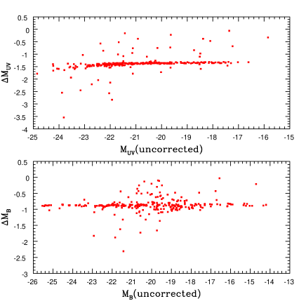
Figure 2: Dust extinction correction as a function of uncorrected absolute magnitude using Calzetti (1997b)’s ‘recipe’. Note that the small scatter arises only because an average $A_{V}=0.97$, $C=0.45$ was applied for those galaxies without direct H$\alpha$ / H$\beta$ extinction measurements.

Figure 3: The relationship between the ratio of H$\alpha$ to UV luminosities and the ionised gas colour excess (from Section 2.2). The left plot is for the fluxes uncorrected for dust extinction (but corrected for stellar absorption), the right plot for fluxes corrected as explained in the text. Only single optical counterpart, field galaxies from SA57 are shown.

The 0.44 factor in Eqn. 6 takes into account the fact that the stars and gas may occupy distinct regions with differing amounts of dust and different dust covering factors. The H$\alpha$ luminosity arises purely from very young, short-lived ionising stars, which must remain close to the (dusty) regions in which they were born. By contrast, the UV continuum at 2000 Å contains a significant contribution from older non-ionising stars, which may no longer be associated with the regions in which they were formed, and hence will suffer less from dust extinction.

If this simple interpretation is correct, then the reddening of the stellar continuum and of the ionising gas should not be strongly correlated; indeed the correlation found (left-hand plot of Fig. 3) is weaker than in previous studies [1994, 1997a]. This may not be an entirely unexpected result. As this survey is selected in the UV at 2000 Å, it is likely to be biased against those objects which are intrinsically dusty and hence have lower measured UV fluxes. Therefore we should not be surprised to see an absence of galaxies with a large H$\alpha$ to UV ratio. Additionally, if the H$\beta$ is suppressed relative to the H$\alpha$ by a significant amount, it will not be measured reliably in the optical spectra, so galaxies with a large $E(B-V)_{g}$ will not be shown in Fig. 3. The trend is similar to that noted by Meurer, Heckman & Calzetti [1999], who plotted the ratio of line flux to F(1600Å) against UV spectral slope, $\beta$, (their Fig. 7), for a sample of local UV-selected starbursts and a sample of 7 $U$-band ‘dropouts’ observed by various authors. These are corrected for Galactic extinction only, and, for the ‘dropout’ galaxies, show only a weak correlation between the line/UV ratios and extinction, similar to that found here.

For the mean correction ($C=0.45$) used above to correct the emission lines, the Calzetti law gives corrections at 2000 Å of $A_{2000}=1.33$. Other studies are in broad agreement with this value, for example Buat & Burgarella [1998] derive $A_{2000}\simeq 1.2$ using radiation transfer models to estimate extinction. Using the parameterization of Seaton [1979], which uses a simple foreground dust screen model, we derive values of $A_{2000}=2.70$ for the average value $C=0.45$. This last correction introduces several complexities. We already have uncomfortably blue colours for a sub-sample of our galaxies; as we shall see in Section 4, there is considerable difficulty in reproducing these using conventional starburst models. The UV luminosities would also become difficult to explain (Section 4). For this reason, we adopt the Calzetti law throughout this paper, noting that although this will result in the smallest corrections to our UV luminosites, due to the nature of the selection criteria for this survey, the UV continuum is not likely to suffer from a larger degree of extinction.

2.3 UV redshift/colour distribution

Figure 4: The redshift distribution for the new sample (left) and the combined sample (right). LEFT: The hatched area is the new SA57 data, while the superimposed heavy shading refers to objects from the Abell 1367 FOCA field. RIGHT: The hatched area is the entire sample, while the heavy shading refers to the restricted sample of galaxies with only one optical counterpart.

Table 7 lists the catalogue for the new observations and the old data. The overall redshift distribution of the new sample can be seen in Fig. 4, together with the distribution of the enlarged sample. The distribution in the new sample has a large peak at $z=0.02$ due to the presence of both the Coma cluster in SA57, and the cluster Abell 1367.

Absolute magnitudes, $M_{UV}$ and $M_{B}$, were derived for each galaxy as follows. The redshift was used to calculate a luminosity distance, and the dust corrected observed colour, $(\mathrm{uv}-\mathrm{b})$, to assign a spectral class and hence $k$ -correction. As in Paper I, the spectral classes were allocated according to the (E/S0, Sa, Sb, Scd, SB) scheme using spectral energy distributions (SEDs) from Poggianti [1997]. The absolute UV magnitude $M_{UV}$ of a galaxy with dust-corrected UV magnitude $m$, redshift $z$, and inferred type $i$, is then computed as:

$$M_{UV}=m_{UV}-5\log d_{L}(z)-25-k_{i}(z)$$ (9)

(and a similar relationship for $M_{B}$) where $d_{L}(z)$ is the luminosity distance at redshift $z$ (we assume $\Omega=1$ and $H_{0}=100~{}\mathrm{h~{}km~{}s^{-1}~{}Mpc^{-1}}$). This allows calculation of the rest-frame colours, $(\mathrm{UV}-\mathrm{B})_{0}$.

Fig. 5 shows the distribution of the $(\mathrm{UV}-\mathrm{B})_{0}$ colours with redshift, with the colours both uncorrected and corrected for dust. Multiple counterpart cases are not shown. Superimposed on these distributions are various model SEDs for different galaxy types as a function of redshift from Poggianti [1997]. The bluer models (labelled SB, as in Paper I) show the colours generated by a starburst superimposed on a passively evolving system. The redder (upper) case, SB1, assumes a 100 Myr burst prior to observation involving 30 per cent of the galaxy mass. The bluer SB2 burst is a shorter (10 Myr) but more massive (80 per cent galaxy mass) burst.

As with previous studies using the FOCA catalogues, including Paper I, there is a significant fraction of galaxies which have extreme $(\mathrm{UV}-\mathrm{B})_{0}$ colours – in this case 12 per cent of the uncorrected colours are bluer than the bluest burst model SED plotted; this increases to 17 per cent after our dust correction. The extreme colours are typically galaxies with strong UV detections, and previous analysis has shown that a systematic offset between the UV and optical photometric systems could not produce effects of the size seen in Fig. 5 (Paper I). An intriguing possibility is that we do not see all of the UV galaxies on the APM plates, which are limited to $\mathrm{b}\simeq 21$. This would suggest that we are not seeing the most extreme objects in the colour plots, as there are no optical counterparts to some of the UV detections. Only deeper optical images of our studied fields can settle this issue. Possible explanations for the objects in our sample with these extreme UV colours will be examined in Sections 3 and 4.

Figure 5: The colour-redshift distribution for the full spectroscopic sample of confirmed galaxies. The photometric system is described in the text. The lines show the model predictions of galaxy colours as a function of redshift for a set of SEDs from Poggianti (1997). These are the same models as in Paper I; see text for full details of these SED models. Multiple counterparts are not shown. The left hand plot shows the colours uncorrected for dust extinction, on the right the colours have been corrected using the Calzetti law.

2.4 The UV, H$\alpha$ and OII luminosity functions revisited

We now update the results of Paper I. The availability of emission line measurements allows us to extend our luminosity functions to those based on H$\alpha$ and [O ii] luminosities as well as the UV flux. With our enlarged sample which reaches $z\simeq 0.4$, we can also test for the presence of evolution internally within our own sample.

We adopt the traditional $\mathrm{V}_{\mathrm{max}}$ method for the luminosity function (LF) derivation (e.g. Felten 1977), corrected for incompleteness in the number-magnitude distribution using the average number counts of Milliard et al. [1992]. The incompleteness function $p(m)$ is defined as the ratio of the number of galaxies with measured spectra to the total number of UV sources per magnitude bin per square degree on the sky.

As in Paper I, we removed sources lying in the redshift range of the intervening Coma and Abell 1367 clusters, which we conservatively take to occupy $0.020<z<0.027$. We also discarded those with insecure optical counterparts. The incompleteness function was computed after these subtractions, as the galaxy number counts of Milliard et al. [1992] are averaged over several fields and therefore we expect the cluster contamination to be sufficiently diluted. The least complete magnitude bin is the faintest ($18\leq m\leq 18.5$), as expected, with $p(m)=65\%$. All other magnitude bins are over 85 per cent complete. The mean incompleteness-corrected $<V/V_{max}>$ is 0.48, i.e. the galaxy distribution can be considered uniform. The volume $V_{max}=p(m)V(z_{max})$ is then defined as the incompleteness-corrected comoving volume at redshift $z_{max}$, out to which the galaxy could have been observed, i.e. satisfying $m(M,z\leq z_{max})\leq 18.5$.

For the H$\alpha$ and [O ii] LFs, the incompleteness function was computed using the new data only, as emission line flux calibration was not available for the old sample. Line widths were measured for $\simeq 74$ per cent of the galaxies in this new sample. However, most of the ‘missing’ lines probably cannot simply be attributed to a low S/N, and we must consider them as truly being absent. For this reason, we do not apply any correction for missing lines to the LFs. Those lines which are unmeasured due to a low S/N, rather than being absent from the spectrum, are, by definition, weak, and therefore ignoring them only adds to the uncertainty at the faint end.

For H$\alpha$, we also account for the fact that the line could not be observed at $z>0.4$, i.e. $z^{\prime}_{max}={\rm min}(z_{max},0.4)$. The [O ii] and H$\alpha$ luminosities have been corrected for extinction as described in Section 2.2. For the UV LF, we consider both the uncorrected and extinction-corrected magnitudes following Calzetti’s prescription as described in Section 2.3.

Fig. 5 shows the effect of the reddening corrections on the colours. After correction, the $(\mathrm{UV}-\mathrm{B})_{0}$ colours are bluer and therefore the galaxy types and $k$-corrections, as inferred from the redshift-colour diagram, will alter slightly. $z_{max}$ will also be slightly lower, as the extinction increases with the emission frequency [1997b] and therefore with redshift. This has a negligible effect on the emission line LFs.

We fit each luminosity function with a Schechter [1976] function in the usual way:

$$\phi(L){\rm d}L=\phi^{\star}\left(L\over L_{\star}\right)^{\alpha}\exp\left(-{L\over L_{\star}}\right){{\rm d}L\over L_{\star}}.$$ (10)

The best fit parameters – $\phi^{\star}$, $\alpha$, $M_{\star}$ for the UV and log $L_{\star}$ for the emission lines – are listed in Table 3, as well as the resulting luminosity densities in each case. These are defined as:

$${\cal L}=\int_{0}^{\infty}L\phi(L){\rm d}L=\phi_{\star}L_{\star}\Gamma(\alpha+2)$$ (11)

The error bars are Poissonian. The four LFs are shown in Figs. 6,7 and 8; we defer discussion of these to $\S$2.5.

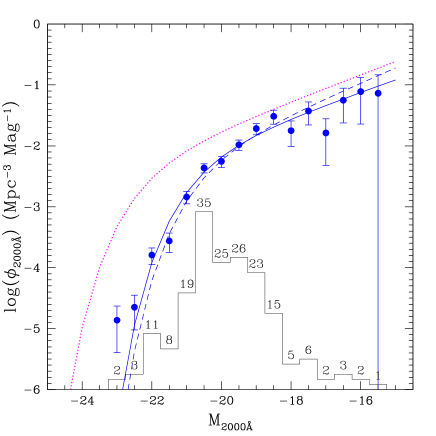
Figure 6: The UV luminosity function derived from the full sample, with (dotted line) and without (solid line and dots) dust extinction correction. The dust correction assumes a Calzetti (1997b) law as described in the text. The long-dashed line is the best fit derived from the old sample (Paper I). The histogram shows the number of galaxies contributing to each magnitude bin in the uncorrected case.

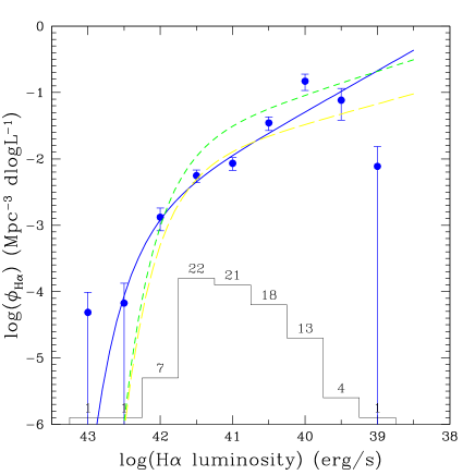
Figure 7: The dust corrected H$\alpha$ luminosity function derived from the present sample. Our best fit is shown by the solid line. The short-dashed line is the H$\alpha$ LF derived by Tresse & Maddox (1998) in a similar redshift range, while the long-dashed line shows the $z\simeq 0$ estimate of Gallego et al. (1995).

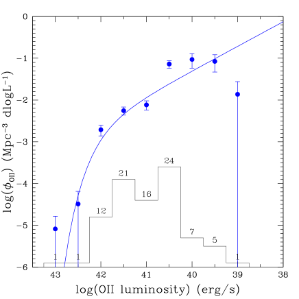
Figure 8: The dust corrected [O ii] luminosity function derived from the present sample (dots). Our best fit is shown by the solid line.

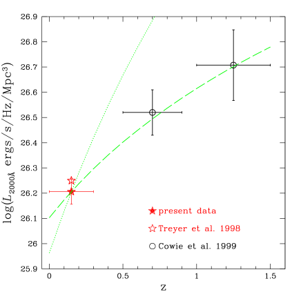
Figure 9: The 2000 Å luminosity density as a function of redshift. Empty dots are from Cowie, Songaila & Barger (1999) extrapolated assuming a faint end slope of -1.5 similar to the present low redshift estimate. The dashed line shows the $(1+z)^{1.7}$ evolution law derived by Cowie et al. The dotted line is a $(1+z)^{4}$ evolution law based on CFRS (Lilly et al. 1996). Both analytic trends are normalised at our new UV estimate; none of the data points are dust corrected.

Parameter	UV uncorrected	UV dust corrected	H$\alpha$	[O ii]
$\alpha$	$-1.51\pm 0.10$	$-1.55\pm 0.11$	$-1.62\pm 0.10$	$-1.59\pm 0.12$
$M_{\star}$/log $L_{\star}$ (cgs)	$-20.59\pm 0.13$	$-22.14\pm 0.20$	$42.05\pm 0.14$	$41.96\pm 0.09$
log $\phi_{\star}$ (Mpc-3)	$-2.02\pm 0.11$	$-2.15\pm 0.14$	$-2.92\pm 0.20$	$-2.82\pm 0.18$
log $\cal L$ (cgs Mpc-3)	$38.08\pm 0.05$	$38.61\pm 0.05$	$39.49\pm 0.06$	$39.46\pm 0.06$
SFR (PEGASE $f=1$)	$-1.52,-1.69,-1.74\pm 0.05$	$-0.99,-1.16,-1.21\pm 0.05$	$-1.56\pm 0.06$	$-1.62\pm 0.05$
SFR (PEGASE $f=0.7$)	$-1.51,-1.68,-1.74\pm 0.05$	$-0.98,-1.15,-1.21\pm 0.05$	$-1.43\pm 0.06$	$-1.47\pm 0.05$

Table 3: Parameters of the best fit Schechter functions for the various luminosity functions. $\cal L$ is the corresponding luminosity density integrated to infinitely faint magnitude. The cgs units are erg/s/Å for the UV luminosity at 2000 Å and erg/s for the H$\alpha$ and [O ii] luminosities. The star-formation rates (SFRs) are derived assuming a Salpeter IMF and the PEGASE code (see section 4 for details). We consider two cases for the fraction of Lyman continuum photons reprocessed into recombination lines ($f=1$ and $f=0.7$ respectively). The three SFRs listed for the UV light densities are taken at 3 different ages of a constant SFH stellar population; the conversion factors are listed Table  4 (first two lines).

Fig. 9 shows the dust uncorrected 2000 Å luminosity density – ${\cal L}$(2000 Å) – as a function of redshift. The high redshift points are from Cowie, Songaila & Barger [1999], although, unlike the authors, we do not assume a faint magnitude cutoff. For consistency, we integrated the Cowie et al. LFs to infinity (Eqn. 11) assuming a faint end slope of -1.5 similar to the present low redshift estimate. The dashed line shows the $(1+z)^{1.7}$ luminosity evolution derived by Cowie et al., normalised at our new UV estimate. As thoroughly discussed by these authors, this evolution is much less radical than the one derived from the CFRS analysis of Lilly et al. [1996] (dotted line, similarly normalised), implying much more star-formation has occured in recent times than previously suspected. In particular, the strong peak in SFR at $z\sim 1-2$ may have been overestimated.

We looked for traces of evolution in the present sample by computing the UV LF in two redshift bins: $[0-0.15]$ and $[0.15-0.4]$. $V_{max}$ is then defined as min$(V(0.15),V(z_{max}))$ for the low redshift galaxies, and as $V({\rm min}(0.4,z_{max}))-V(0.15)$ for the higher redshift bin. The mean redshifts in each bin are 0.078 and 0.22 respectively. The low and high redshift LFs overlap around $M_{\star}$ and both are consistent with the best fit derived for the full sample. Therefore no statistically significant evolution can be seen in the present data. However, the increase in light density between the mean redshifts of the two samples expected from a $(1+z)^{1.7}$ evolution law, as derived by Cowie et al., is only a factor of 1.2 – within the error bars of the present estimate. By contrast, the $(1+z)^{4}$ evolution law based on the CFRS by Lilly et al. [1996] predicts a 60 per cent increase in UV light density between the two redshift bins, which is difficult to reconcile with our statistics, assuming the Poisson fluctuations are the dominant source of uncertainty. Although the present data do not allow a very reliable conclusion on this point, a weak rate of evolution for the UV light density seems more likely.

2.5 The low-redshift star-formation rate

The uncorrected UV LF is in good agreement with the estimate of Paper I, although the latter was based on a third of the present number of redshifts. The steep faint end slope remains a significant feature, in contrast with local optically-selected surveys. It is also apparent in the H$\alpha$ and [O ii] LFs, although the faintest data points were excluded in both cases and the fits are relatively poor. A steep faint end slope is also found in the 1.4 GHz LF derived from faint radio galaxies [1999, 1998] confirming the preponderance of star-forming galaxies among this population. The shape of our H$\alpha$ LF is in poor agreement with previous low-redshift determinations (Gallego et al. 1995, Tresse & Maddox 1998), although given the large uncertainties in emission line measurements, the fact that the three estimates derive from very different selection criteria, and that they probe different redshift ranges, the discrepancy is probably acceptable. Our integrated H$\alpha$ luminosity density is $\sim 43$ per cent lower than the Tresse & Maddox [1998] value derived from a sample of $I$-band selected galaxies at $z<0.3$ from the CFRS. The mean redshift of this sample is 0.2. Truncating the present UV-selected sample at redshift 0.3 leaves the best fit H$\alpha$ LF practically unchanged, while slightly reducing the mean redshift to 0.12. The discrepancy still cannot be reasonably attributed to evolution within such a short redshift range, rather to poor statistics, differing selection effects and possibly $k$-correction models (used in computing $V_{max}$). Our H$\alpha$ luminosity density is also $\sim 27$ per cent higher than the estimate of Gallego et al. [1995], which probes a more local ($z=0$), and also probably more comparable (H$\alpha$ selected), galaxy population. The rate of evolution resulting from the latter discrepancy (from $z=0$ to 0.15) is actually in very good agreement with that derived by Cowie et al. [1999] from the 2000 Å light density.

The conversion from UV, H$\alpha$ or [O ii] luminosity densities into SFRs is very model dependent (see Section 4 for a detailed discussion). As an illustration, we use the PEGASE stellar population synthesis code [1997] with which we were able to derive the conversion rates for all three diagnostics self-consistently. We assume a Salpeter IMF with stellar masses ranging from 0.1 – 120 ${\rm M}_{\odot}$, and consider two cases for the fraction of Lyman continuum photons reprocessed into recombination lines ($f=1$ and $f=0.7$ respectively). These models are described in detail in Section 4. The conversion factors are listed in Table 4 (first two lines).

The H$\alpha$ and [O ii] luminosity densities thus converted into SFRs give very consistent results. The conversion factors we use here yield SFRs $\sim$ 30 to 40 per cent higher than those derived from Madau (1998)’s fiducial model based on the stellar population synthesis code of Bruzual & Charlot (1993) (for a similar IMF). As our H$\alpha$ luminosity density falls between the values of Gallego et al. [1995] and of Tresse & Maddox [1998], so does the resulting SFR for a given stellar population synthesis model.

Converting UV light into an instantaneous SFR is less straightforward as it involves an uncertain contribution from longer-lived stars, adding to the already large uncertainty in the dust corrections. We consider three different ages (in a constant star-formation history) to derive the UV conversion factors; 10, 100 and 1000 Myr (see Section 4 for details – the conversion factors are as listed in Table 4). The range of SFRs thus derived from the 2000 Å light density is shown in Fig. 10, along with the present (dust-corrected) and previous H$\alpha$ and [O ii] estimates. The left and right panels assume $f=1$ and $f=0.7$ respectively. Also shown is the local SFR estimate recently derived from 1.4 GHz data [1998, 1999].

The SFR derived from the UV continuum uncorrected for dust extinction is in good agreement with the corrected H$\alpha$ and [O ii] estimates for the case $f=1$, and slightly lower than these values for $f=0.7$. Taking the emission line estimates at face value, this suggests that local UV-selected galaxies are not significantly affected by dust and that Calzetti’s extinction law in the UV is significantly overestimated for this population. There are many caveats however, not least of which is the model-dependency of the conversion factors from line/UV luminosities to SFRs (see, for example, Schaerer [1999]). The H$\alpha$ extinction corrections may be underestimated, as argued by Serjeant et al. [1998] based on their estimate of the local SFR from radio emission, which is dust insensitive. Our Balmer-derived dust corrections to the H$\alpha$ and [O ii] lines are certainly likely to be lower limits, as discussed in Section 2.2. It is also possible that the H$\alpha$ and UV luminosities are measured over different effective apertures, though we consider this unlikely (see Section 4.2 for a discussion of this point).

The large uncertainties involved in determining the low redshift SFR are readily apparent from the large scatter both in the data and in the models. These uncertainties tend to increase with redshift, making interpretations about the SFR evolution quite unreliable at this point. Understanding the detailed physical mechanisms of star-formation is therefore a crucial task towards reconciling the various SF diagnostics and finally drawing conclusions about the nature of star formation in the nearby Universe.

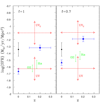
Figure 10: The local star-formation rate derived from the present and other local surveys, assuming the conversion factors described in the text (previous H$\alpha$ estimates are rescaled according to these factors). All the emission line estimates are dust-corrected as described in the text. The triangle represents the H$\alpha$ estimate of Gallego et al. (1995) and the diamond that of Tresse & Maddox [1998]. The present estimates are indicated by error bars. The lower cross shows the range of SFRs estimated from the uncorrected UV continuum light (assuming the range of models described in the text), while the upper dotted one shows the dust-corrected values. The H$\alpha$ and [O ii] estimates are where indicated on the plot. The $z=0$ dot shows the SFR from the 1.4 GHz analysis of Serjeant et al. [1998].

3 Emission line properties

A significant advance over the spectra presented in Paper I is that we now have reliable line measurements for a substantial fraction of the UV-selected sample. For the highest S/N spectra, EWs and fluxes for up to 5 emission lines have been measured (6 including the deblended [N ii] line). Our analysis now proceeds in two parts. This section will cover the emission line properties and correlations, together with diagnostic diagrams, whilst the next section will cover comparisons of emission lines with the UV fluxes and the subsequent star-formation modelling.

One of the possible explanations for the abundance of extreme $(\mathrm{UV}-\mathrm{B})_{0}$ colour objects seen in this survey is that the UV light produced in these galaxies comes from a non-thermal source, such as an QSO/AGN. The mean (not dust-corrected) $\mathrm{UV}-\mathrm{B}$ colour of the 23 such objects in our sample is -1.41, though there is large scatter, with some as blue as $\simeq-4$. Clearly, care must be taken to remove such objects from our ‘star-forming’ galaxy sample. Those galaxies with obvious AGN characteristics have been removed from the sample; however, there remains the possibility that AGNs with strong star-forming components have remained in the sample, giving over-abundant UV fluxes. While the best way to assess the size of the effect is to image the galaxies in the UV and look at the distribution of the UV light, an indirect method of identifying AGN from starburst galaxies is to use emission line diagnostic diagrams.

Figure 11: The diagnostic diagrams as described in the text, for both the corrected and uncorrected fluxes. Typical $1\sigma$ error bars are shown in the top right. Note how the reddening corrections move many more galaxies away from the H ii region, though the error bars are larger.

Diagnostic diagrams can be used to separate and distinguish between different ionisation sources in the host galaxies. Considering the lines measured in this survey, the [O iii]/H$\beta$ versus [O ii]/H$\beta$ diagram is the most appropriate to use. Though not an ideal choice, as the ratio of [O ii]/H$\beta$ depends significantly on reddening, this diagram allows us to look at what proportion of our sources may have ionisation sources other than hot OB-type stars, which is vital given the star-formation modelling attempted in Section 4. Fig. 11 shows this diagnostic diagram for both the reddened and unreddened fluxes. The line on the diagram is taken from Tresse et al. [1996], and shows the approximate empirical limit between H ii galaxies and ‘active’ galaxies.

It is interesting to note that a significant fraction of the sources lie to the right of the line in Fig. 11, i.e. away from the region that is normally associated with H ii galaxies. The important point however is the size of the uncertainties on the plot, particularly in the corrected fluxes. Though not shown on the diagram, the points to the right of the line typically have larger errors – up to 2 times as high – so it is difficult to conclude that a large fraction of the sources have a strong AGN component. Additionally, the effect of stellar absorption on the H$\beta$ line has a large effect on this plot, adding to the uncertainty involved. Although the H$\beta$ fluxes include some allowance for the H$\beta$ absorption due to the way in which they were measured, some individual points may still contain significant errors associated with them. Any further correction will increase the measured H$\beta$ flux, moving the galaxy down and to the left on the diagram, back into the H ii galaxy region.

If galaxies that lie away from the H ii region are responsible for the extreme $(\mathrm{UV}-\mathrm{B})_{0}$  colours seen in this survey, then we expect a correlation between the [O ii]/H$\beta$ ratio and UV-B colour; none is found. This suggests that an explanation of the $(\mathrm{UV}-\mathrm{B})_{0}$ colours cannot be found purely in the source of ionisation of the galaxies, at least not with the current quality of data.

Another possible explanation for the anomalous UV colours compared to the model predictions could be unusually low metallicities in the galaxies concerned. To investigate this, we examined the metallicity using the $R_{23}$ emission line index [1979] following the prescription from Poggianti et al. [1999]. This is defined in terms of corrected fluxes as:

$$R_{23}=\frac{(\mathrm{\hbox{[O\,{ii}]}}_{3727}+\mathrm{\hbox{[O\,{iii}]}}_{4959,5007})}{\mathrm{H}_{\beta}}$$ (12)

and is calibrated using:

$$12+\log(\frac{\mathrm{O}}{\mathrm{H}})=9.265-0.33x-0.20x^{2}-0.21x^{3}-0.33x^{4}$$ (13)

where $x=\log(R_{23})$. Full details of this calibration can be found in Zaritsky, Kennicutt & Huchra [1994]; in brief, the absolute $R_{23}$ index calibration is accurate only to $\simeq 0.2~{}\mathrm{dex}$, so this estimator is most useful for calculating relative metallicities.

Only the SA57 galaxies – the more complete spectroscopic sample – were used in this analysis, creating a sub-sample of 35 galaxies that have the complete line information required to estimate the metallicity. An added complication is the effect of stellar absorption on the H$\beta$ line, as the metallicity estimates are very sensitive to this; however, due to the emission line nature of our survey galaxies, and they way in which the H$\beta$ fluxes were measured, the effect of stellar absorption should not be a large one.

Figure 12: Plot of the metallicity derived from the R₂₃ index against $(\mathrm{UV}-\mathrm{B})_{0}$ and H$\alpha$ luminosity for the SA57 galaxies which have the complete line information. Coma galaxies are plotted as squares, field galaxies are stars.

Fig. 12 shows the relationship between galaxy colour, H$\alpha$ luminosity and metallicity. Those galaxies which are members of the Coma cluster are plotted as empty squares, the field galaxies are shown as stars. There is a slight suggestion in the left hand plot that the bluer galaxies have a higher metallicity (a counter-intuitive result). There is no apparent correlation with H$\alpha$ luminosity. Unfortunately, due to the significant errors on the points (not shown) it is difficult to conclude a great deal about metallicity being responsible for the extreme $(\mathrm{UV}-\mathrm{B})_{0}$ colours seen in some of our galaxies.

To conclude, there is still no single convincing explanation for the abnormal colours that we see in this survey on the basis of the emission line information that we have at our disposal. While it is difficult to completely rule out the possibility of significant AGN contamination, or metallicity effects, the evidence is not strong. Improved S/N ratios must be obtained on the relevant lines to finally settle the issue.

4 Star Formation Modelling

4.1 Discussion of spectral evolution models

Our UV selected galaxy survey allows us to compare two different tracers of star-formation activity which should, when converted, produce similar SFRs. The follow-up optical spectra have provided H$\alpha$ emission line measurements, and the FOCA experiment has provided a measurement of the UV continuum at 2000 Å. This UV continuum light is dominated by short-lived, massive main-sequence stars, with the number of these stars proportional to the SFR. H$\alpha$ emission lines are generated from re-processed ionising UV radiation at wavelengths of less than 912 Å. This radiation is only produced by the most massive stars, which have short lifetimes of $\simeq$ 20 Myr. To convert these two tracers into actual SFRs for each galaxy requires constructing the spectral energy distribution (SED) of a model galaxy over time, and the following method is used.

The spectral characteristics of an instantaneous burst of star-formation for a given IMF and set of evolutionary stellar tracks are calculated, and, using a time-dependent SFR, then used to build synthetic spectra over the course of a galaxy’s history. This time-varying SED is converted into time-varying UV magnitudes and H$\alpha$ luminosities (or EWs). For the UV magnitudes, the response (or transmission) of the FOCA-2000 Å filter is included. For H$\alpha$, the emission line flux can be calculated from the number of ionising Lyman continuum photons, assuming that a certain fraction of these photons are absorbed by the hydrogen gas in the galaxy. This gas is assumed to be optically thick to the Lyman photons (according to case B recombination).

The number of ionising photons is assumed to be a fraction $f$ of the number of Lyman continuum photons, and two values will be assumed here. The first is $f=0.7$, as proposed by DeGioia-Eastwood [1992], who studied H ii regions in the LMC. However, when the galaxy as a whole is studied, the fraction absorbed is much higher (see Kennicutt [1998] for a discussion). Leitherer et al. [1995] studied the redshifted Lyman continuum in a sample of 4 starburst galaxies with the Hopkins UV telescope, and reports that $<3$ per cent are not absorbed, i.e. $f=1$. These absorbed ionising photons are then re-processed into recombination lines; for H$\alpha$ we adopt a conversion of 0.45 H$\alpha$ photons per ionising Lyman photon.

There are several galaxy spectral synthesis models available in the literature (see Leitherer et al. [1996] for a recent review). Different models predict slightly different time-varying SEDs, and therefore different conversion factors. For H$\alpha$, produced only by the most massive stars, a constant star-formation history (SFH) will have little time-dependence in H$\alpha$ luminosity – for the published models, the H$\alpha$ luminosity reaches a constant level after $\simeq 20-30~{}\mathrm{Myr}$, and varies little thereafter. However, the conversion factor is very sensitive to the form of the IMF, as it depends critically on the number of high-mass stars. The conversion from UV continuum luminosity to a star-formation rate (SFR) is more difficult, as the UV continuum at 2000 Å also contains a contribution from stars with a longer lifetime, and, unlike H$\alpha$, will not settle at a constant level but will increase slowly with time. Three different conversion factors will be used here, for ages of 10, 100 and 1000 Myr.

There are many H$\alpha$ conversion factors given in the literature (e.g. Glazebrook et al. [1999], Kennicutt et al. [1998] and Madau et al. [1998] for discussions). The modelling in this paper makes use of two spectral synthesis codes: PEGASE (see Fioc and Rocca-Volmerange [1997] for further details), and Starburst 99, developed by Leitherer et al. [1999]. The PEGASE code uses the evolutionary tracks of Bressan et al. [1993], together with the stellar spectral libraries assembled by Fioc and Rocca-Volmerange, and is limited to solar metallicity. These libraries cover the wavelength range of 200 Å to $10\mu$m with a resolution of 10 Å. Full details of the tracks used in the Starburst 99 code can be found in Leitherer et al. [1999]. This code has a choice of 5 metallicities ($\mathrm{Z}=0.040$, 0.020 ($=\mathrm{Z}_{\odot}$), 0.008, 0.004 and 0.001).

The H$\alpha$ and UV conversion values used are taken from Madau et al. [1998], Kennicutt [1998] and directly from the PEGASE and Starburst 99 spectral synthesis codes, and tabulated in Table 4 for a SFR of $1\mathrm{M_{\odot}yr}^{-1}$ and a Salpeter [1955] IMF. The table also lists various [O ii] conversion factors used in Section 2.4. While the UV continuum is relatively insensitive to the fraction of Lyman ionising photons absorbed by the nebular gas, the H$\alpha$ fluxes are critically sensitive to this poorly known number; values of $f=0.7$ and $f=1$ were used to produce the two PEGASE values. The SB99 UV conversion factors do not increase with decreasing metallicity for the 10 Myr case (as would be expected) due to red supergiant (RSG) features appearing in the population; this metallicity dependent feature is due to the inability of most evolutionary models to predict correctly RSG properties on this time-scale (see Leitherer et al. [1999] for a full discussion).

Source	Assumed Salpeter IMF	L(H$\alpha$)	L([O ii])	L(UV2000)
	lower/upper mass limits	($10^{41}\mathrm{erg~{}s}^{-1}$)	($10^{41}\mathrm{erg~{}s}^{-1}$)	($10^{39}\mathrm{erg~{}s}^{-1}\AA^{-1}$)
	($\mathrm{M}_{\odot}$)			10 Myr	100 Myr	1000 Myr
PEGASE ($f=1.0$)	0.1/120	1.15	1.25	4.01	5.90	6.69
PEGASE ($f=0.7$)	0.1/120	0.85	0.88	3.94	5.84	6.63
SB99 (Z=0.040)	0.1/120	1.23		3.53	5.01
SB99 (Z=0.020)	0.1/120	1.53		3.44	5.17
SB99 (Z=0.004)	0.1/120	1.79		3.55	5.69
SB99 (Z=0.001)	0.1/120	2.01		3.46	5.85
M98	0.1/125	1.58			6.00
K98	0.1/100	1.27	0.71

Table 4: The conversion rates used to transform H$\alpha$  [O ii] and FOCA UV₂₀₀₀ luminosities into SFRs (in the sense $\mathrm{L}=SFR\times\mathrm{conversion~{}factor}$). Values from Madau et al. [1998], Kennicutt [1998], and the PEGASE and Starburst 99 spectral synthesis models.

Figure 13: The correlation between the H$\alpha$ and FOCA-UV luminosities, for the most secure sample. Only field galaxies are shown. Left: Both luminosities uncorrected, right: both luminosities corrected. Errors are $1\sigma$. The lines show the position of galaxies with a constant SFR. The lines are (from left to right) SOLID:PEGASE $f=0.7$ and $f=1.0$, SHORT DASHED: Starburst 99, metallicities 0.04, 0.02, 0.004, 0.001, LONG DASHED: M98 H$\alpha$ with PEGASE UV $f=1.0$. UV conversion factors taken at 100 Myr. The markers refer to SFRs of 0.1, 1.0, 10 and 100 M${}_{\odot}~{}\mathrm{yr}^{-1}$ respectively for the PEGASE $f=0.7$ and $\mathrm{Z}=0.001$ Starburst 99 models. See text for further details.

4.2 The star-formation diagnostic plots

For a constant star formation history, SFRs calculated from the two different tracers should produce the same result. Fig. 13 shows the correlation between the H$\alpha$ and UV luminosities from the most secure sample, for both uncorrected (left) and dust corrected (right) data. The overlaid lines show the conversion into SFRs using the different factors in Table 4. As can be seen, though there is a good correlation over three orders of magnitude, the different range of SFH parameters cannot reproduce the scatter around the correlation. The other trend is that the majority of the data points lie above the constant SFH lines, i.e. the galaxies are typically over-luminous in the UV for a given H$\alpha$ luminosity. This result is also reflected in the integrated SFRs derived from the H$\alpha$ and UV light densities (Section 2). In this case, although Fig. 10 does not show the uncorrected H$\alpha$ derived value against the uncorrected UV value, it clearly shows the large discrepancy between the corrected H$\alpha$ and UV derived SFRs. It also shows that the corrected H$\alpha$ derived SFR is only slightly above the uncorrected UV derived SFR, (also seen in Fig. 14 for individual galaxies, a point returned to later).

The significance of the scatter can be examined by comparing with that expected from the random measurement errors. The data points are fitted using a least-squares technique, and the distribution of the residual ($\log(\mathrm{L}_{H\alpha})$ – ‘least-squares best-fit $\log(\mathrm{L}_{H\alpha})$’) compared with the distribution of the $\log(\mathrm{L}_{H\alpha})$ errors. While the distribution of the $\log(\mathrm{L}_{H\alpha})$ errors peaks strongly at $\simeq 0.05~{}\mathrm{to}~{}0.1$, the distribution of the residuals is flat over a much larger range (0 to 1). A similar pattern is seen in the $\log(\mathrm{L}_{\mathrm{UV}})$ errors. An explanation for the scatter must therefore be sought elsewhere.

A possible systematic effect which could explain the large UV flux relative to the H$\alpha$ flux concerns the relevant apertures over which the two measurements were made. The finite (2.7″) diameter of the WYFFOS fibres implies that some of the galaxy light may be lost from the spectra, especially if the UV magnitudes were measured over a larger aperture. Unfortunately due to the poor imaging resolution of the FOCA detector, most UV sources are unresolved and therefore we do not have any reliable size information. However, we do not believe this effect to be a serious one. Firstly, inspection of the POSS images suggests that a diameter of 2.7″ will include all of the continuum light from most of our galaxies. Secondly, if this were to be a significant effect, we would expect the ratio of UV luminosity to H$\alpha$ luminosity to decrease with redshift as more of the galaxy light is included in the WYFFOS fibres. We examined the data for such a trend, but found no significant trend from $z=0$ to $z=0.3$. From this, we conclude there to be no evidence for significant aperture mismatches internally within our sample.

The over-luminosity in the UV and the scatter cannot be explained in terms of simple foreground screen dust corrections, as these will increase the discrepancy, not reduce it. Other dust geometries are also unlikely to be the cause. To move the observed positions of the galaxies so that they agree with the constant SFH predictions requires large dust corrections to the H$\alpha$ luminosities, but almost negligible corrections for the UV luminosities. Though the $C=0.45$ correction derived in Section 2.2 applied solely to the H$\alpha$ fluxes produces a better agreement between the two SFR tracers, to remove the scatter completely would require corrections of up to $C=1.4$, corresponding to $\mathrm{A}_{\mathrm{V}}\simeq 3$ (see Section 2.2), whilst simultaneously having no effect on the UV luminosities. Such corrections are not seen from the Balmer decrement measurements, and would require extreme dust geometries.

This trend initially appears to contradict that of Glazebrook et al. [1999], who find that their H$\alpha$ derived SFRs lie above that derived from the UV continuum at 2800 Å. As a comparison, Fig. 14 shows both our sample and that of Glazebrook et al. converted to SFRs on an individual galaxy basis using the appropriate PEGASE conversion factor at 2800 Å (taken from Table 3, Glazebrook et al. [1999]). The dust corrections applied to the H$\alpha$ and the 2800 Å UV are as given in Glazebrook et al. It is clear that only the bright end of our galaxy population is sampled by Glazebrook et al., and that in this range there is a good agreement between the two samples. The dashed line shows a perfect agreement between H$\alpha$ and UV derived SFRs, and it is clear that correcting just the H$\alpha$ luminosities for dust reduces the offset apparent in Fig. 13, indicating that our UV corrections may be upper limits and possibly overestimated, though the scatter is more difficult to explain.

However, both the offset and the scatter in Fig. 13 and the lower (dust corrected) half of Fig. 14 can also be explained by a series of starbursts superimposed on underlying galactic SFHs. During a starburst, a galaxy moves up and to the right on the UV-H$\alpha$ plane, increasing luminosity in both quantities. As the burst decays, the H$\alpha$ rapidly decreases due to the short lifetimes of ionising stars, but the UV luminosity is temporarily retained, moving the galaxy to the left. Subsequently, the galaxy returns to its pre-burst (quiescent) position, describing a loop on the plot.

Figure 14: A comparison of SFRs derived from our sample (open squares) and that of Glazebrook et al. 1999 (stars). SFR conversions are taken from the PEGASE program. The dashed lines shows a perfect agreement between H$\alpha$ and UV SFRs. TOP: Only H$\alpha$ fluxes are corrected for dust, BOTTOM: Both UV and H$\alpha$ corrected. There is a good agreement between the samples, though the Glazebrook et al. sample only covers the bright end of our distribution.

This scenario can also reconcile the difference between bright galaxies, including the Glazebrook et al. sample, where the H$\alpha$ SFR $>$ UV SFR, and the fainter sample in the lower half of Fig. 14, where the opposite is seen. The bright galaxies are (likely) at the peak of a particular burst, and, in a Calzetti-like dust scenario, the UV will contain a contribution from young massive (and hence dust obscured stars) as well as older (less obscured) stars; hence our UV corrections are probably underestimated in this range and the H$\alpha$ SFR will be larger then UV derived measures. As the burst dies away, the contribution to the UV luminosity from the obscured massive stars decreases and the UV SFR will become larger than the (more rapidly decaying) H$\alpha$ SFR. The next section attempts to quantify the burst parameters in this picture.

At this point it is relevant to return to the vexing question of the origin of the extreme $(\mathrm{UV}-\mathrm{B})_{0}$ colours. Fig. 15 plots the H$\alpha$ EW against $(\mathrm{UV}-\mathrm{B})_{0}$ for the galaxies in the UV photometric system (see Section 2.2 for details). Only those galaxies for which errors in the H$\alpha$ EWs are available with an unambiguous optical identification are shown. This removes some galaxies with extreme $(\mathrm{UV}-\mathrm{B})_{0}$ $\simeq-4$ colours where the UV fluxes were possibly the sum of two galaxies, and were therefore anomalously bright when compared to the $B$ magnitudes. The advantage of this diagnostic plot is that it has no complications due to uncertainties in the flux calibration of the WHT optical spectra.

The galaxies plotted in Fig. 15 represent two different environments – cluster members in Abell 1367 or Coma (squares), and field galaxies (crosses). The plot shows a clear trend – the strongest H$\alpha$ emission systems are the bluest systems. Most of the galaxies tend to cluster at around $\mathrm{H}\alpha\simeq 20-60$, $(\mathrm{UV}-\mathrm{B})_{0}\simeq 0$, but there are two other areas on this plot of interest. One consists of those galaxies with very blue $(\mathrm{UV}-\mathrm{B})_{0}$ colours of $\simeq-2~{}\mathrm{to}~{}-4$, the other are those with a significant H$\alpha$ EW ($\simeq 50-100$) but much redder colours.

Figure 15: Plot of H$\alpha$ EW against $(\mathrm{UV}-\mathrm{B})_{0}$ colours for field and cluster galaxies in SA57 (COMA) and Abell 1367, overlaid with various SFHs using different IMFs. Field galaxies shown as crosses, cluster galaxies as open squares. Colours have been dust corrected. The solid line is the Rana-Basu IMF (also circle markers), short dash Scalo IMF (also triangles) and long dash Salpeter IMF (squares). The markers refer to different galaxy ages (0.5, 6 and 12 Gyr).

In order to distinguish between the cluster SFH and field SFH, Fig. 15 also shows various predictions according to the PEGASE spectral synthesis program. The histories are for exponential bursts of the form:

$$\mathrm{SFR}=\tau^{-1}\exp\left(-\frac{t}{\tau}\right)$$ (14)

where $\tau$ is the characteristic time of the SFH, and is equal to 1.25 Gyr. Altering this value does not change the trajectory, only the speed at which a galaxy travels along it. The plot shows that the cluster galaxies are solely responsible for the group of galaxies that have redder colours and a significant H$\alpha$ emission.

The effect of varying the IMFs on the colours is also explored. A wide range of IMFs are available, and three are shown in Fig. 15; these are the Scalo [1986], Salpeter [1955] and Rana-Basu [1992] IMFs. As in Fig. 13, it is clear that these SFHs are incapable of reproducing the scatter in the observed points of Fig. 15, even when variations in the IMF are considered, and certainly cannot reproduce the $(\mathrm{UV}-\mathrm{B})_{0}$ colours seen here.

In summary, smoothly declining SFHs cannot a) reproduce the UV colours and luminosities seen in the field galaxies, b) produce the strong H$\alpha$ emission seen in the relatively red cluster galaxies, or c) generate the scatter seen in both Figs. 13 & 15.

4.3 Modelling the luminosities and colours

In this section, we aim to understand the scatter in Fig. 13 by examining the duty cycle of star formation in the survey galaxies. We adopt throughout this section the Salpeter [1955] IMF with mass cut-offs at $0.1~{}\mathrm{M}_{\odot}$ and $120~{}\mathrm{M}_{\odot}$. The modelling techniques discussed here were also attempted using other IMFs – those also used in Section 4.2 – as well as varying the mass-cutoffs used; however, no appreciable difference was obtained using these ‘standard’ IMFs.

In a method similar to that adopted by Glazebrook et al. [1999], who suggested that the SF in a sample of 13 CFRS $z\simeq 1$ galaxies is erratic, we will examine the effect of superimposing a set of bursts on a smoothly declining star formation history. We ask what range in the strength and duration of the bursts is required to reproduce the scatter observed.

In order to check the bursting hypothesis as a solution for the scatter in Fig. 13 (and Fig. 15), the positions of non-bursting galaxies should ideally be plotted as a ‘reality check’ on the model predictions. In the absence of UV data for a large sample of normal galaxies, this test cannot yet be done. Meanwhile it must be assumed that the absolute positions of galaxies predicted by the synthesis codes are correct, and that there is no systematic offset when comparing model and observations.

To model the properties of a galaxy, a series of bursts of varying mass (M) and burst decay time ($\tau$) were superimposed on gradual declining or constant SFHs. This gives three free fitting parameters: M, $\tau$, and the number of bursts, $N_{b}$, as well as the form of the declining SFH. Several versions of the latter were tried; two are introduced here, which differ in the resulting present-day colour. Their characteristics are summarised in Table 5.

The models are compared to the observed data points statistically. We first examined a maximum likelihood method. The likelihood, $L$, of the observed galaxy points being drawn from a particular model is given by (Glazebrook et al. [1999]):

$$L=\prod_{i}\int\int\frac{P(h,u)\exp(-\frac{(h_{i}-h)^{2}}{2\Delta h^{2}_{i}}-\frac{(u_{i}-u)^{2}}{2\Delta u^{2}_{i}})}{2\pi\Delta h_{i}\Delta u_{i}}{\rm d}u{\rm d}h$$ (15)

where the observational H$\alpha$ and UV luminosities are represented by $u_{i}$ and $h_{i}$ respectively for each galaxy $i$, $\Delta u_{i}$ and $\Delta h_{i}$ are the observational uncertainties in these points measured from the individual spectra ($\Delta h_{i}$) or based on the UV magnitudes ($\Delta u_{i}$, Section 2.1), $u$ and $h$ represent the parameterization of the PEGASE model points, and $P(h,u)$ is the probability density of a particular model point in H$\alpha$ / UV space.

SFH	$\tau$ (Gyr)	$(\mathrm{UV}-\mathrm{B})_{0}$	H$\alpha$ EW	$\mathrm{L}(\mathrm{H}\alpha)$	$\mathrm{L}(UV_{2000})$
				$10^{40}\mathrm{erg~{}s}^{-1}$	$10^{39}\mathrm{erg~{}s}^{-1}\AA^{-1}$
1 (Red)	2.00	1.37	1.6	0.0105	0.149
2 (Blue)	5.00	-0.58	17.1	0.1540	2.018

Table 5: The two exponential SFHs on which the bursts were superimposed. Superpositions were made between galactic ages of 4 to 12 Gyr; the characteristics above are taken at 12 Gyr.

The bursts were added at random times from a galactic age of 4 to 12 Gyr, and were fitted to the data points for the period 8 to 12 Gyr. We then calculated the likelihood of a SFH matching the observed data points. This was repeated 100 times, and the mean likelihood obtained.

Two types of burst were considered; the first was a burst of constant strength over its duration, the other was an exponentially declining burst similar in form to Equation 14. Constant strength bursts generally gave lower likelihoods as they tend to generate stationary points in H$\alpha$ / UV space; exponential bursts generate more scatter. The ‘most likely’ burst parameters for each galaxy type are listed in Table 6. A typical likelihood contour plot is shown in Fig. 17. Little improvement was obtained by varying the number of bursts; a value of 20 was used throughout, equivalent to a burst every $\simeq 400~{}\mathrm{Myr}$. The best-fitting bursts are also demonstrated graphically in Fig. 16, where the path of the model galaxy in H$\alpha$ /UV space is superimposed on the data. As can be seen, these bursts reproduce many of the observed data points but do not reproduce the scatter.

Test	SFH	Burst $\tau$	Burst Mass	Nb
		(Myr)	(% galaxy mass)
1	Red	130	25-30	20
1	Blue	50	10-15	20
2	Red	50	3-7	20
2	Blue	70	15-20	20

Table 6: The parameters for the ‘best-fit’ bursts for the two galaxy SFHs. The top parameters are those generated by maximum likelihood, the bottom are those from the second statistical test, which concentrates on reproducing the scatter seen in the observed points.

Figure 16: Two distributions of UV-H$\alpha$ measures for the sample (crosses) compared to that for model galaxies, found by superimposing a series of bursts on the SFHs described in Table 5 using the best-fit parameters of Table 6 (only the ‘redder’ galaxy is shown). The open squares show the track made by a global exponentially declining SFR, forming a total mass of $10^{10}~{}\mathrm{M}_{\odot}$, as described in the text. The lines show the paths described by a ‘model’ galaxy during its evolution. LEFT: Maximum likelihood ‘best-fit’. Much of the observed scatter is not reproduced by this model. RIGHT: The second statistical test, with the emphasis on matching the scatter in the plot, rather than maximising the likelihood.

A second, simpler statistical approach was adopted. The aim is to assess the number of observed points that could be reproduced by the maximum likelihood fits. This simply counted the number of data points reproduced by a particular SFH. Fig. 17 shows an example contour plot from this method, Table 6 lists the parameters of the ‘best-fitting’ histories as before, and Fig. 16 shows these histories graphically.

Although the burst parameters for the two methods are similar for the blue galaxy, they are very different for the first (redder) galaxy. The maximum likelihood method favours longer bursts. With a short burst the galaxy spends much of its lifetime away from the position of the observed points; the underlying component is red and the galaxies were selected in the UV.

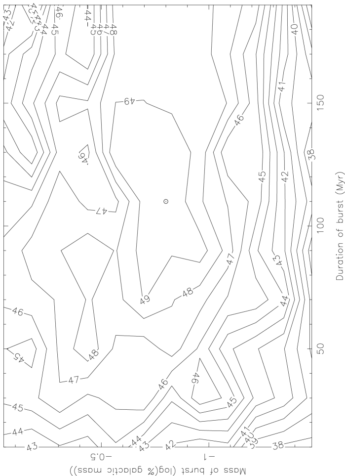
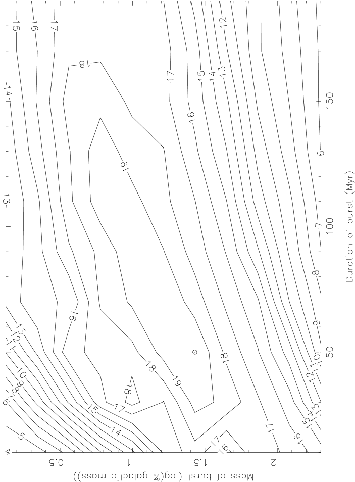
Figure 17: Examples of the burst mass/duration contour plots. LEFT: A maximum likelihood contour plot. The peak is at $\tau=130$ Myr, M$\simeq 30$%. RIGHT: The contours generated by the alternative statistical test, which reproduces more of the scatter in the points. The peak is at $\tau=50$ Myr, M$\simeq 5$%. Both plots are for the redder SFH from Table 5.

It can also be seen that the histories do not reproduce the highest UV luminosity galaxies; these are the galaxies that have the strongest $(\mathrm{UV}-\mathrm{B})_{0}$ colours. In Section 3, we concluded that there was no conclusive evidence that the anomalously bright $(\mathrm{UV}-\mathrm{B})_{0}$ colours could be explained by AGN contamination or metallicity effects. We find that the best-fit histories from above could neither generate the scatter nor the bluest colours seen in the data. Though the highest UV luminosity bursts are reproducible via short, intense bursts (Fig. 18), the extreme $(\mathrm{UV}-\mathrm{B})_{0}$ colours are still not attained.

Figure 18: As Fig. 16, but attempting to reproduce the high UV luminosity points. This shows $\tau=10$ Myr, 15% mass bursts. The UV luminosity points can be reproduced, but even these histories are not capable of reproducing the extreme $(\mathrm{UV}-\mathrm{B})_{0}$ colours found in this survey.

5 Discussion

We have seen that the scatter in the UV-H$\alpha$ plane is consistent with a star formation history that is complex and erratic. The fundamental observation is that most of our UV-selected galaxies show excess UV luminosities when compared to their H$\alpha$ fluxes on the assumption of a simple star formation history. Moreover, dust extinction would serve to enhance the difference, not reduce it unless, perhaps, the spatial distribution of dust is particularly complex. In Section 4, we considered more complex star formation histories invoking a regular pattern of bursts on top of more general exponentially-declining histories and found that the different time-dependencies of the stars that produce UV flux and excite nebular emission can reproduce the scatter observed.

It is interesting to compare this result with those (very few) surveys for which two star formation diagnostics are available. Using different selection criteria, Glazebrook et al. [1999] (13 targets colour selected from the $I$-limited CFRS) and Yan et al. [1999] (slitless HST NICMOS spectroscopy of 33 targets) both find H$\alpha$ derived SFRs in excess of those from UV measurements (at 2800 Å) - the opposite effect to that seen here. They attribute their discrepancy primarily to dust extinction [1999, 1999] but also discuss an erratic SFH [1999]. The effect of dust extinction in these different samples is very difficult to quantify; however both of these surveys sample only the bright end of our galaxy sample, and we have shown there is actually good agreement between these surveys and ours in this range. The other major difference of significance is the size of the samples available for analysis and the quality of spectral data involved; clearly both are better for our low $z$ sample than in the $z>1$ analyses.

The nature of our UV selected galaxies can also be assessed by considering comparisons with 1.4 GHz radio continuum detections. This radiation, caused by synchrotron radiation from relativistic electrons, is thought to be generated by electrons accelerated by supernovae from massive ($\mathrm{M}>5\mathrm{M}_{\odot}$) short-lived stars, and therefore should be a further tracer of the SFR in galaxies [1992]. A literature search revealed three radio surveys which cover some or all of SA57 – the FIRST catalogue [1997], the NVSS [1998] – both using the VLA – and Windhorst, Heerde & Katgert [1984], which uses the Westerbork Synthesis Radio Telescope. The correlations between these surveys and the FOCA detections are shown in Fig. 19.

Though the radio catalogues correlate well, there is a surprisingly poor correlation with the FOCA sources. Only 3 FIRST sources and 1 NVSS source have FOCA counterparts within $20\arcsec$ – a generous search radius – and H$\alpha$ was detected in only one of these. However, converting 1.4 GHz luminosity to SFR for our adopted IMF [1998, 1998]:

$$\mathrm{SFR_{1.4}(M\geq 0.1M_{\odot})}=\frac{L_{1.4}}{7.45\times 10^{20}\mathrm{~{}W~{}Hz^{-1}}}\mathrm{M_{\odot}yr^{-1}}$$ (16)

we find that the largest SFRs in our UV-selected sample ($\simeq 15\mathrm{M_{\odot}yr^{-1}}$) would give expected 1.4 GHz luminosities at $z=0.1$ of only $\simeq 2\mathrm{mJy}$, i.e. close to the detection threshold of the FIRST survey ($\simeq 1\mathrm{mJy}$). None the less, as many sources should lie closer than $z=0.1$, we might have expected more 1.4 GHz detections. As previous studies [1998] have shown that even dust corrected H$\alpha$ luminosity underestimates local SFRs when compared with 1.4 GHz observations, this lack of correlation may indicate that the H$\alpha$ derived SFRs are marginally overestimated. Deeper 1.4 GHz surveys are required to explore this further.

Figure 19: The correlations between FIRST, NVSS and Windhorst et al. (1984) 1.4 GHz radio surveys and the FOCA 2000 Å detections. FOCA sources are shown as open squares, FIRST as square crosses, NVSS as diagonal crosses and Windhorst as open circles. A poor correlation between FOCA sources and radio detections is observed.

Although we have shown that the excess UV luminosities can be reproduced by considering bursting SFHs, we have generally failed to reproduce the full range of $(\mathrm{UV}-\mathrm{B})_{0}$ colours for our sample; in general, colours smaller than $(\mathrm{UV}-\mathrm{B})_{0}\simeq-2$ are problematic to generate, and we cannot easily explain a number of intense UV sources which are optically faint. In Paper I we eliminated trivial explanations for this category of sources including photometric discrepancies between the FOCA and POSS ($B$) magnitude systems. It is certainly possible to generate UV-optical colours more extreme than the Poggianti starburst SEDs. For example, using the Starburst 99 code [1999], $(\mathrm{UV}-\mathrm{B})_{0}\simeq-2.5$ – $-3$ can be generated (but only on a very short time-scales) using standard IMFs and smaller ($10^{4}~{}\mathrm{Myr}$) timesteps then the Poggianti SEDs ($10^{7}~{}\mathrm{Myr}$). The number of such sources found then can only be understood in the context of more detailed modelling of the SF duty cycle. On the whole, however, it is becoming apparent that we do not understand the SEDs of these systems well.

The burst duty cycle produces results consistent with that of earlier workers. The original analysis of Glazebrook et al. [1999] adopted slightly longer and more massive bursts. Marlowe, Meurer & Heckman [1999] examined the nature of starbursts in dwarf galaxies and found similar burst parameters. They find such bursts typically account for only a few per cent of the stellar mass. Theoretical studies [1996] suggest that the burst durations may be shorter than those found here, as well as being more intense in terms of stellar mass. A comprehensive study of bursts in irregular galaxies has also been undertaken by Mas-Hesse & Kunth [1999]. They also find that star-formation episodes are essentially short, with a mean age of around 4 Myr. Though this is much shorter than the ‘best-fit’ duty cycles found in this survey, it does correlate well with the bursts that we require in order to reproduce the full range of UV luminosities ($\simeq 10~{}\mathrm{Myr}$).

There remain many avenues for further investigation into the nature of star-formation in local samples of field galaxies. There is an urgent need for resolved images so that the morphological details and physical location of the star forming regions can be determined. Ultimately, only such images can rule out significant AGN components in the most extreme UV sources in our sample. Secondly, more accurate UV photometry is needed over more bandpasses to check for dust and SED differences. Finally, we comment in our analysis of the importance of verifying and constraining the various stellar synthesis models in the UV against a control sample of quiescent objects with well-behaved star formation histories. The absence of such a body of data simply highlights our surprising ignorance of the UV properties of normal galaxies.

6 Conclusions

We sought, in this paper, to illustrate very simply how little is known about the star formation properties of the bulk population of field galaxies with $z<0.4$. For a well-defined population of UV-selected sources, for which detailed spectroscopic analyses have been carried out, we have found:

1. A volume-density of star formation well in excess of previous estimates both when using the UV and H$\alpha$ luminosity functions. The UV luminosity function has a remarkably steep faint end slope making optical redshift surveys prone to underestimating the luminosity density at modest redshift.

2. No evidence, internally within our sample, for a strong increase in UV luminosity density with redshift, such as would be expected on the basis of earlier work based on the CFRS (Lilly et al. 1996).

3. A significant fraction of UV sources have UV-optical colours at the extreme limit of those reproducible in starburst models, and some are beyond this limit. From detailed emission line studies, we find no evidence for AGN contamination or anomalous metallicities in these sources.

4. The star formation rates derived from UV flux and extinction-corrected H$\alpha$ line measurements are not consistent in the framework of model galaxies with smoothly-declining star formation histories. We find the UV luminosities are consistently higher than expected and dust effects would only exacerbate this discrepancy.

5. We also find a significant scatter in the UV-H$\alpha$ plane and can reproduce this (and the offset discussed above) in terms of a duty cycle of starbursts superimposed upon longer term histories. We discuss ways of physically constraining such a model and produce illustrative examples where 5–20% of the galactic mass is involved in bursts with decay time $\tau\simeq 50~{}\mathrm{Myr}$ and a frequency of one every $\simeq 400~{}\mathrm{Myr}$.

Table 7: The updated UV-z catalogue. ‘OC’ indicates the number of optical counterparts on the POSS plates within 10$\arcsec$. The position (1950) is that of the closest optical counterpart. ‘T’ is the galaxy type, classified on the basis of UV-B colour; $\mathrm{T}=1-8$ refers to types E, S0, Sa, Sb, Sc, Sd, SB1 & SB2. All colours are rest-frame and dust corrected. H$\alpha$ and H$\beta$ give rest-frame EWs.

OC	RA	DEC	uv	z	Oii	H$\alpha$	H$\beta$	T	$\mathrm{M}_{UV}$	$(\mathrm{UV-B})_{0}$	Comments
SA 57
1	13:06:32.16	+29:48:38.2	16.55	0.0228	16.2	21.8	5.0	3	-18.10	1.63	OII,wOIII,sH$\beta$,sH$\alpha$
1	13:06:46.29	+29:43:37.9	16.89	0.1130	25.3	36.0	5.5	6	-21.70	-0.52	OII,H$\beta$,H$\alpha$,HK
1	13:06:50.23	+29:40:26.7	17.20	0.2430	13.7	18.2	2.1	4	-23.07	0.33	OII,HK,H$\alpha$
1	13:06:07.71	+29:46:05.6	18.21	0.2800	0.0	0.0	0.0	4	-22.86	0.52	OII
1	13:06:30.66	+29:39:30.4	17.95	0.2285	64.1	118.4	0.0	8	-22.50	-2.79	OII,H$\beta$,OIII,H$\alpha$
1	13:06:07.74	+29:44:40.2	17.74	0.0241	96.5	96.4	22.0	5	-17.23	-0.46	OII,H$\beta$,OIII,H$\alpha$,H$\gamma$
1	13:05:07.10	+30:00:23.6	17.58	0.4020	0.0	0.0	0.0	8	-24.01	-4.48	OII,OIII,H$\alpha$
1	13:05:21.88	+29:55:46.3	18.34	0.0663	0.0	0.0	0.0	4	-19.52	0.22	OII
1	13:07:21.56	+29:22:45.6	17.87	0.1420	0.0	0.0	0.0	8	-21.54	-4.12	HK
1	13:06:51.43	+29:27:27.7	18.18	0.4820	0.0	0.0	0.0	8	-23.79	-4.13	HK
1	13:06:07.65	+29:36:35.6	18.29	0.1227	24.7	71.6	7.0	5	-22.04	-0.44	OII,HK,H$\alpha$
2	13:06:36.80	+29:28:41.0	18.33	0.2110	0.0	0.0	0.0	8	-21.94	-3.85	HK
1	13:04:25.82	+30:00:58.3	17.41	0.1465	0.0	0.0	0.0	8	-22.06	-2.58	OII
2	13:07:05.26	+29:11:28.8	16.94	0.0627	71.7	73.0	17.6	6	-20.16	-0.58	OII,H$\beta$,OIII,H$\alpha$
1	13:05:00.02	+29:40:04.3	16.09	0.0176	37.0	71.3	9.9	5	-18.49	0.00	OII,HK,H$\beta$,OIII,H$\alpha$
1	13:04:15.30	+29:51:58.9	18.49	0.1752	6.7	12.5	0.0	6	-21.45	-0.64	HK, H$\alpha$
2	13:05:16.43	+29:35:22.5	17.74	0.3203	49.2	405.6	0.0	8	-23.44	-4.46	OII,OIII,H$\alpha$
1	13:03:49.57	+29:58:56.5	17.89	0.3348	20.0	77.2	10.4	8	-25.20	-3.77	H$\alpha$,OII,HK
1	13:07:04.39	+29:02:33.2	17.31	0.1350	31.9	0.0	0.0	5	-22.06	-0.13	OII
1	13:05:01.46	+29:34:48.4	18.38	0.1717	28.2	46.4	0.0	8	-21.43	-3.52	OIII,H$\alpha$
1	13:05:49.35	+29:21:16.6	16.94	0.1170	0.0	0.0	0.0	4	-22.14	0.37	HK;noisy;
1	13:03:39.69	+29:56:17.2	17.95	0.1790	0.0	0.0	0.0	6	-22.04	-1.05	OII
1	13:04:14.72	+29:44:32.4	17.67	0.0846	4.4	11.1	0.0	6	-20.71	-1.00	HK, H$\alpha$
1	13:06:48.52	+29:02:35.2	17.33	0.0211	119.4	37.6	10.3	5	-18.02	-0.30	OII,H$\beta$,OIII,H$\alpha$
1	13:06:23.47	+29:08:47.4	15.98	0.0609	56.6	13.9	0.0	3	-21.71	1.73	OII,HK,wOII,H$\alpha$
1	13:06:21.20	+29:08:58.6	17.23	0.2640	0.0	0.0	0.0	8	-23.56	-3.12	noisy;HK
2	13:05:38.28	+29:18:00.1	18.12	0.1441	16.1	15.1	0.0	7	-21.34	-1.55	OII,HK,H$\alpha$
2	13:05:23.08	+29:21:27.4	17.31	0.1131	95.9	0.0	31.2	8	-21.62	-3.67	OII,H$\beta$,OIII,H$\alpha$,H$\gamma$
2	13:05:22.71	+29:21:19.6	17.31	0.1260	0.0	0.0	0.0	8	-21.84	-4.33	HK
1	13:03:29.88	+29:51:59.4	16.78	0.0558	8.0	8.8	0.0	3	-20.72	1.74	HK,OIII,H$\alpha$
2	13:04:13.54	+29:39:51.1	18.29	0.0892	35.6	54.7	9.5	8	-20.15	-2.37	OII,H$\beta$,OIII,H$\alpha$
2	13:04:53.91	+29:27:21.2	17.89	0.5213	61.3	0.0	99.6	8	-24.22	-4.09	OII,OIII,H$\beta$
1	13:05:40.80	+29:14:43.1	16.47	0.0800	0.0	33.7	7.2	4	-21.80	0.41	OII,OIII,H$\alpha$,H$\beta$
1	13:04:09.89	+29:37:58.8	16.04	0.0246	0.0	17.1	3.4	2	-19.77	2.50	wOII,H$\beta$,OIII,H$\alpha$
1	13:04:37.54	+29:29:21.4	17.85	0.1673	48.0	65.6	11.9	5	-20.92	-0.28	OII,H$\beta$,OIII,H$\alpha$
1	13:03:37.14	+29:44:00.2	18.03	0.0511	30.1	20.4	3.5	4	-18.73	0.47	OII,HK,wOIII,H$\beta$,H$\alpha$
1	13:04:23.45	+29:30:37.4	18.07	0.0697	0.0	11.8	0.0	7	-19.87	-1.54	wOII,H$\alpha$
1	13:03:48.44	+29:40:05.1	17.24	0.1817	86.2	300.1	22.9	7	-21.43	-1.75	OII,H$\beta$,OIII,H$\alpha$
1	13:06:11.39	+29:00:41.8	16.84	0.0558	30.6	18.1	3.7	5	-20.64	-0.38	OII,HK,H$\alpha$,H$\beta$,OIII
2	13:04:22.12	+29:29:59.3	18.22	0.1821	10.2	0.0	0.0	6	-21.81	-1.03	HK,OII
1	13:03:52.02	+29:38:00.4	17.07	0.0244	78.4	26.4	0.0	4	-18.61	0.10	OII,OIII,H$\alpha$
1	13:05:55.86	+29:02:53.4	17.24	0.0394	44.1	53.6	8.2	6	-19.65	-1.07	OII,H$\beta$,OIII,H$\alpha$,HK
1	13:03:32.85	+29:41:38.0	18.39	0.1837	0.0	0.0	0.0	7	-21.60	-1.54	OII,HK
1	13:02:53.21	+29:51:18.0	16.26	0.0236	45.0	33.3	7.4	3	-18.38	1.10	OII,H$\beta$,OIII,H$\alpha$
2	13:03:40.30	+29:37:37.9	18.06	0.2859	129.8	0.0	0.0	8	-22.90	-4.20	OII,OIII,wH$\beta$
1	13:02:43.94	+29:52:15.3	18.25	0.1850	42.2	69.9	11.7	7	-21.12	-1.50	OII,H$\beta$,OIII,H$\alpha$,HK
1	13:05:48.77	+29:01:33.6	17.89	0.1176	39.0	37.7	9.4	8	-21.12	-2.85	OII,OIII in sky
1	13:04:33.69	+29:21:34.7	18.00	0.1817	13.2	84.85	3.1	8	-22.72	-2.42	OII,HK,H$\alpha$
1	13:06:27.44	+28:50:05.1	17.08	0.1650	0.0	0.0	0.0	8	-22.65	-2.90	OII
1	13:05:19.98	+29:08:21.6	18.54	0.3913	21.0	111.2	8.4	8	-22.27	-2.70	OII,HK,wH$\alpha$
2	13:06:04.39	+28:55:59.2	18.12	0.1970	0.0	0.0	0.0	7	-22.02	-1.51	z=.197
1	13:02:40.62	+29:49:55.6	17.61	0.4080	0.0	0.0	0.0	8	-24.01	-3.38	HK
2	13:05:29.52	+29:03:20.2	17.82	0.2471	0.0	0.0	0.0	8	-22.81	-3.13	HK,Mgb,wOII
2	13:05:30.34	+29:03:16.3	17.82	0.2475	45.3	114.3	16.7	8	-23.88	-3.31	OII,H$\beta$,OIII,H$\alpha$
1	13:04:29.07	+29:17:29.9	18.36	0.2424	30.5	62.5	0.0	8	-22.22	-3.22	OII,OIII,H$\alpha$
1	13:02:38.07	+29:46:52.4	18.35	0.1861	15.5	65.2	3.4	7	-23.81	-1.96	OII, HK, H$\alpha$
1	13:06:03.45	+28:49:13.9	17.47	0.1151	41.8	24.0	0.0	5	-21.56	-0.15	OII,abn,wH$\alpha$
1	13:05:32.05	+28:57:31.5	18.40	0.0566	27.1	24.9	2.4	5	-19.11	-0.24	OII,HK,OIII,H$\alpha$
1	13:04:23.62	+29:15:48.9	16.63	0.0616	36.2	50.1	9.4	6	-21.21	-0.51	sOII,H$\beta$,OIII,H$\alpha$
1	13:05:26.55	+28:58:41.3	16.90	0.0702	9.6	8.0	0.0	4	-21.09	0.37	OII,abn,wH$\alpha$
2	13:02:57.71	+29:38:39.1	18.35	0.1858	0.0	0.0	0.0	8	-21.64	-2.73	OII,HK,H$\alpha$: OII
2	13:02:30.70	+29:45:16.1	17.95	0.0480	0.0	0.0	0.0	8	-19.17	-2.49	HK
1	13:03:28.24	+29:25:25.9	17.33	0.2416	17.6	23.5	3.8	8	-22.38	-2.36	OII,OIII,H$\alpha$,abn
2	13:05:28.03	+28:52:01.4	17.55	0.1860	25.0	0.0	0.0	8	-22.44	-2.52	OII,HK,H$\alpha$
1	13:02:00.66	+29:47:57.0	18.06	0.2235	85.2	100.0	15.6	8	-22.34	-2.47	OII,H$\beta$,OIII,H$\alpha$
2	13:04:00.52	+29:14:47.2	17.18	0.2849	23.4	180.1	9.8	8	-23.65	-4.62	OII,H$\beta$,OIII,H$\alpha$
1	13:04:10.95	+29:11:04.1	18.07	0.0613	47.2	39.4	0.0	6	-19.61	-1.12	OII,OIII,H$\alpha$
2	13:02:09.94	+29:43:33.8	17.18	0.0230	0.0	0.0	0.0	8	-18.35	-2.44	H$\alpha$,OIII,wOII,H$\beta$
1	13:02:12.45	+29:42:24.8	18.05	0.0650	0.0	0.0	0.0	8	-19.72	-3.56	HK
1	13:04:50.67	+28:58:14.8	18.14	0.2474	51.4	76.6	0.0	8	-22.49	-2.81	OII,H$\beta$,OIII,H$\alpha$
1	13:02:06.14	+29:42:07.9	18.37	0.2403	76.0	89.9	8.7	8	-23.16	-3.44	OII,H$\beta$,OIII,H$\alpha$
2	13:02:48.95	+29:30:12.8	17.38	0.0230	0.0	0.0	0.0	6	-18.16	-0.85	OIII,H$\alpha$,wOII,H$\beta$
1	13:02:15.80	+29:38:34.0	16.87	0.3040	0.0	0.0	0.0	8	-24.22	-2.60	HK
1	13:04:48.41	+28:54:49.3	17.95	0.0397	56.3	45.8	8.1	7	-18.51	-1.80	OII,OIII,H$\alpha$,abs,H$\beta$
2	13:03:09.04	+29:21:37.1	18.06	0.1270	0.0	0.0	0.0	7	-21.13	-1.71	wS/N,abn
1	13:04:07.33	+29:05:10.8	17.80	0.0799	20.2	16.2	0.0	4	-20.47	0.33	OII,HK,H$\alpha$
2	13:04:19.63	+29:00:19.0	17.51	0.4010	0.0	0.0	0.0	8	-24.07	-4.62	HK,OII
2	13:04:19.78	+29:00:26.9	17.51	0.1126	29.1	48.4	7.0	6	-21.53	-0.69	OII,HK,H$\beta$,H$\alpha$
1	13:04:28.46	+28:57:50.8	17.92	0.3880	28.9	157.1	10.8	8	-23.59	-2.57	OII,H$\beta$,OIII,H$\alpha$
1	13:01:41.45	+29:42:43.6	17.91	0.3398	67.0	0.0	24.1	8	-23.36	-2.74	OII, OIII
1	13:04:00.52	+29:04:38.0	17.49	0.0930	0.0	0.0	0.0	7	-21.05	-2.00	HK
1	13:02:26.87	+29:29:58.1	17.25	0.1389	0.0	18.6	0.0	5	-22.18	-0.22	OII,H$\alpha$,HK,vwOII
2	13:05:04.61	+28:46:37.0	18.05	0.1151	35.3	36.6	0.0	7	-20.94	-1.45	OII,HK,H$\alpha$
2	13:04:37.52	+28:53:13.7	17.45	0.0480	0.0	0.0	0.0	8	-19.67	-4.76	HK
1	13:03:09.40	+29:16:44.0	16.59	0.0176	5.1	17.4	0.0	1	-18.52	4.01	HK,abs,H$\alpha$,sS/N
2	13:01:55.86	+29:35:55.8	18.32	0.0492	0.0	0.0	0.0	8	-18.85	-3.82	OII
2	13:01:55.26	+29:36:03.0	18.32	0.1861	0.0	0.0	0.0	8	-21.67	-2.58	OII,HK,H$\beta$,H$\alpha$
1	13:01:41.32	+29:39:36.8	18.18	0.1667	49.0	64.8	11.9	6	-21.49	-0.74	OII,H$\beta$,OIII,H$\alpha$
2	13:02:56.12	+29:18:53.6	18.11	0.0178	35.2	100.6	15.7	6	-15.85	-1.14	OII,OIII,H$\alpha$,H$\beta$
1	13:03:21.92	+29:08:18.0	15.41	0.0268	37.0	42.2	6.4	3	-21.93	1.00	OII,OIII,H$\alpha$,H$\beta$
1	13:04:25.49	+28:50:20.3	17.39	0.0828	0.0	0.0	0.0	4	-20.95	0.14	HKabs,H$\alpha$
1	13:04:09.89	+28:53:20.3	17.84	0.6695	264.6	0.0	49.9	8	-24.85	-4.28	OII,H$\beta$,OIII
1	13:02:11.57	+29:25:28.0	18.14	0.0896	66.6	38.0	9.6	7	-19.66	-2.07	OII,H$\beta$,OIII,H$\alpha$
1	13:02:13.53	+29:24:51.9	17.47	0.0195	17.3	14.0	0.0	4	-17.72	0.23	OII,OIII,H$\alpha$
1	13:04:32.93	+28:46:14.5	17.26	0.0828	7.3	0.0	0.0	3	-21.10	1.27	HK,broad H$\alpha$,wOII
1	13:02:14.19	+29:21:01.9	17.90	0.1799	125.9	183.4	28.2	8	-22.02	-2.29	vsOII,H$\beta$,OIII,H$\alpha$
1	13:04:16.43	+28:47:04.0	17.94	0.0270	5.9	8.9	0.0	3	-17.97	1.71	HK,H$\alpha$
1	13:04:51.57	+28:36:35.6	16.29	0.0186	34.3	9.1	0.0	3	-18.80	1.76	abs,H$\alpha$,wOII,wOIII
1	13:01:05.01	+29:38:00.2	18.16	0.0500	0.0	0.0	0.0	8	-19.05	-3.83	HK
1	13:02:47.46	+29:07:09.6	18.02	0.1781	90.1	181.5	20.9	8	-22.47	-2.88	OII,H$\beta$,OIII,H$\alpha$
1	13:02:15.16	+29:14:25.5	16.48	0.0254	31.1	32.1	4.4	4	-19.25	0.68	OII,OIII,H$\alpha$,H$\beta$
1	13:04:25.24	+28:38:42.3	18.38	0.1863	35.2	69.7	6.8	8	-21.14	-2.33	OII,OIII,H$\alpha$,H$\beta$
1	13:02:45.39	+29:04:56.9	17.06	0.1861	23.3	47.2	5.1	6	-23.53	-0.62	OII,H$\beta$,OIII,H$\alpha$
1	13:00:49.01	+29:34:15.4	17.11	0.0835	18.3	19.4	2.0	6	-22.00	-0.53	OII,H$\beta$,OIII,H$\alpha$
1	13:00:53.53	+29:31:42.1	17.58	0.0817	20.9	27.0	4.1	5	-21.12	-0.36	OII,H$\alpha$,HK
1	13:03:48.16	+28:43:55.0	15.85	0.0676	92.8	60.9	11.5	4	-22.05	0.58	OII,H$\beta$,OIII,H$\alpha$
1	13:03:45.03	+28:43:35.2	16.06	0.0679	38.4	65.7	10.3	4	-22.03	0.45	OII,OIII,H$\alpha$,H$\beta$
1	13:04:02.91	+28:37:54.6	17.02	0.0393	7.6	8.1	0.0	5	-19.69	-0.07	HK,abs,H$\alpha$,wOIII
1	13:02:51.82	+28:53:38.2	16.97	0.0218	36.6	25.7	4.0	4	-18.52	0.14	OII,H$\beta$,OIII,H$\alpha$
1	13:00:59.29	+29:22:49.2	17.55	0.0825	22.6	20.3	3.6	4	-19.64	0.73	OII,HK,OIII,H$\alpha$
1	13:02:42.78	+28:54:32.0	17.75	0.0184	49.8	54.5	7.8	4	-17.43	0.69	OII,OIII,H$\alpha$,H$\beta$
1	13:01:53.07	+29:07:07.0	17.52	0.0254	74.1	104.3	22.8	6	-18.47	-0.93	OII,OIII,H$\alpha$,H$\beta$
1	13:03:01.48	+28:48:32.0	18.33	0.1170	30.0	33.6	0.0	5	-20.73	-0.04	OII,H$\alpha$,HK
1	13:01:59.06	+29:04:42.8	14.25	0.0267	40.3	47.1	6.9	2	-21.99	3.20	OII,OIII,H$\alpha$,H$\beta$
2	13:01:33.44	+29:10:37.6	18.03	0.1978	11.8	23.6	0.0	6	-22.19	-0.81	wOII, HK, H$\alpha$
2	13:01:32.86	+29:10:34.5	18.03	0.0760	0.0	0.0	0.0	8	-20.07	-3.90	H$\alpha$ only
1	13:02:05.41	+29:01:54.8	18.20	0.0268	26.9	24.1	4.1	7	-17.67	-1.54	OII,OIII,H$\alpha$
2	13:02:55.68	+28:48:03.4	18.25	0.1645	25.0	0.0	0.0	8	-21.47	-2.72	OII,vwH$\beta$,OIII,H$\alpha$
1	13:03:31.77	+28:36:53.0	18.09	0.1759	0.0	160.1	0.0	8	-21.78	-2.63	OIIwOIII, H$\alpha$
2	13:01:58.51	+29:01:55.0	17.48	0.0184	0.0	79.7	21.5	7	-17.51	-1.44	wOII,H$\beta$,OIII,H$\alpha$
1	13:01:05.21	+29:15:22.6	17.80	0.0830	0.0	0.0	0.0	3	-20.57	1.99	HK,H$\alpha$
1	13:02:25.99	+28:51:14.9	18.16	0.2532	78.0	113.8	16.9	6	-21.67	-0.95	OII,H$\beta$,OIII,H$\alpha$
1	13:02:15.28	+28:53:47.1	15.48	0.0570	4.1	6.3	0.0	2	-22.28	3.17	HK,vwOII,H$\alpha$
1	13:02:11.95	+28:53:43.2	15.95	0.0224	27.0	38.3	4.2	3	-20.02	1.87	OII,abs,OIII,H$\alpha$,H$\beta$
1	13:01:58.98	+28:55:49.6	18.46	0.2798	0.0	27.6	0.0	8	-22.46	-2.29	HK,abs
1	13:02:41.80	+28:42:17.0	18.73	0.2187	14.9	50.1	0.0	4	-21.74	0.38	OII,abs,H$\alpha$,H$\beta$, OIII
1	13:02:33.29	+28:43:05.3	17.60	0.0696	28.5	27.4	5.8	5	-20.24	-0.32	OII,OIII,H$\alpha$,H$\beta$
2	13:02:08.38	+28:46:55.4	18.53	0.0370	0.0	0.0	0.0	8	-18.03	-3.68	z:,HK
1	13:01:49.26	+28:48:37.7	16.00	0.0273	59.6	47.0	17.9	5	-19.92	-0.32	OII,H$\beta$,OIII,H$\alpha$
1	13:01:07.18	+28:57:30.8	16.83	0.0224	15.1	35.3	5.1	6	-17.36	-0.80	wOII,H$\beta$,OIII,H$\alpha$
Abell 1367
1	11:41:52.98	+20:47:39.8	17.48	0.0965	0.0	0.0	0.0	6	-21.18	-0.93	OII,HK, OIII
1	11:42:30.43	+20:42:57.5	16.49	0.0231	0.0	23.1	0.0	1	-19.24	5.86	H$\alpha$,HK,H$\beta$abn
1	11:41:28.99	+20:45:35.4	18.19	0.0669	26.4	21.2	0.0	6	-19.68	-1.17	OII,HK,H$\beta$,OII,H$\alpha$
1	11:40:59.21	+20:46:04.6	16.91	0.1687	30.9	95.67	11.5	4	-22.96	0.36	OII,H$\beta$,OIII,H$\alpha$
1	11:42:53.69	+20:40:01.9	17.91	0.0821	14.8	17.1	0.0	4	-20.41	0.31	wOII,HK,OIII,H$\alpha$
1	11:42:58.57	+20:39:27.8	17.48	0.1129	10.6	33.1	3.1	3	-21.55	1.31	OII,HK,H$\beta$,H$\alpha$
1	11:42:02.60	+20:42:14.0	16.53	0.0391	27.6	10.5	0.0	2	-20.34	2.52	wOII,HK,H$\alpha$
2	11:42:57.11	+20:36:32.9	17.26	0.0480	0.0	0.0	0.0	3	-19.91	1.56	HK,z:
1	11:41:26.28	+20:39:30.9	16.76	0.0399	77.1	82.9	14.5	3	-20.00	1.32	OII,H$\beta$,OIII,H$\alpha$
1	11:41:12.18	+20:38:27.7	17.30	0.0222	0.0	0.0	0.0	1	-18.34	3.90	HK,H$\alpha$+b in abn
1	11:40:54.03	+20:38:39.9	18.22	0.2084	7.2	49.0	0.0	5	-22.12	-0.15	OII,HK,H$\alpha$
1	11:43:21.82	+20:27:28.1	16.93	0.0815	7.1	16.6	1.0	4	-21.38	0.75	wOII,HK,sH$\alpha$
1	11:40:40.45	+20:34:40.5	17.22	0.1770	0.0	0.0	0.0	3	-22.79	1.87	HK,z:
1	11:41:02.34	+20:32:20.4	17.02	0.0413	36.7	37.6	0.0	7	-19.79	-1.47	OII,HK,OIII,H$\alpha$
1	11:41:13.29	+20:31:34.6	16.51	0.0205	89.2	199.2	40.4	3	-18.79	1.81	OII,H$\gamma$,H$\beta$,OIII,H$\alpha$
1	11:40:22.05	+20:34:08.2	17.45	0.0700	0.0	0.0	0.0	4	-20.53	0.09	H$\beta$,H$\alpha$
1	11:42:16.91	+20:27:56.5	18.38	0.0243	0.0	0.0	0.0	4	-17.29	0.26	HK,H$\gamma$,H$\alpha$,H$\beta$e+a
1	11:41:41.45	+20:29:54.4	15.91	0.0216	0.0	10.2	0.0	1	-19.67	5.53	H$\alpha$,HK,H$\beta$(abn)
1	11:43:04.16	+20:22:49.6	18.52	0.3826	22.4	49.4	10.4	8	-22.96	-3.78	OII,H$\beta$,OIII,H$\alpha$
1	11:41:22.60	+20:27:44.9	15.63	0.0220	16.2	64.1	5.3	1	-19.99	3.83	OII,HK,H$\beta$,OIII,H$\alpha$
1	11:42:11.59	+20:24:09.7	15.39	0.0214	13.9	0.0	0.0	1	-20.16	5.13	H$\beta$abn,HK,wOII,H$\alpha$
2	11:40:24.84	+20:29:35.5	18.07	0.0706	65.3	24.6	0.0	8	-19.87	-2.25	OII,OIII,H$\alpha$
1	11:41:56.61	+20:23:02.9	18.08	0.0240	26.9	92.5	14.6	2	-17.68	2.83	OII,H$\beta$,OIII,sH$\alpha$
1	11:40:48.41	+20:25:49.3	17.45	0.0707	53.9	73.6	13.6	6	-20.54	-1.14	OII,H$\beta$,OIII,H$\gamma$,H$\alpha$
1	11:42:07.45	+20:21:20.2	17.80	0.0885	15.0	15.8	0.0	7	-20.64	-1.76	OII,HK,OIII,H$\alpha$
1	11:41:23.40	+20:21:16.6	14.97	0.0250	5.1	12.0	0.0	1	-20.94	4.30	wOII,HK,H$\alpha$
1	11:41:01.40	+20:21:04.4	17.48	0.0684	44.4	61.8	13.0	7	-20.42	-1.71	OII,H$\gamma$,H$\beta$,OIII,H$\alpha$
1	11:41:08.38	+20:19:19.9	18.15	0.0692	7.4	15.5	0.0	6	-19.79	-0.52	OII,HK,H$\alpha$
1	11:41:18.49	+20:16:31.8	17.36	0.0966	4.2	3.5	0.0	6	-21.30	-0.90	OIII,HK,H$\alpha$
1	11:40:09.47	+20:18:35.4	15.65	0.0289	0.0	0.0	0.0	1	-20.60	4.81	HK,H$\alpha$,H$\beta$abs
1	11:39:39.87	+20:19:34.2	16.26	0.0204	16.7	17.5	1.3	2	-19.13	2.33	OII,HK,OIII,H$\alpha$
1	11:42:40.08	+20:09:19.8	17.62	0.0814	0.0	0.0	0.0	5	-20.68	-0.12	abn:HK,H$\beta$,wH$\alpha$
1	11:42:19.65	+20:09:28.8	17.63	0.0818	11.4	22.1	23.7	5	-20.68	-0.29	OII,HK,OIII,H$\alpha$
1	11:41:51.04	+20:10:44.6	18.48	0.2460	0.0	0.0	0.0	8	-22.14	-3.35	HK,z:
1	11:40:20.70	+20:14:37.2	15.02	0.0244	28.8	38.1	4.6	2	-20.78	2.91	OII,HK,H$\beta$,OIII,H$\alpha$
1	11:40:03.61	+20:14:47.5	17.01	0.0245	98.4	53.7	8.7	5	-18.67	-0.02	OII,H$\beta$,OIII,H$\alpha$
1	11:41:20.91	+20:10:20.7	16.87	0.0214	0.0	0.0	0.0	1	-18.68	5.15	abn:HK,G,H$\beta$,others
1	11:39:38.39	+20:15:09.9	15.53	0.0261	21.2	16.8	0.0	2	-20.42	3.73	OII,wHK,OIII,H$\alpha$
1	11:40:18.41	+20:13:05.5	18.11	0.1318	44.8	121.6	11.3	8	-21.14	-3.20	OII,H$\beta$,OIII,H$\alpha$
2	11:42:25.90	+20:05:34.0	18.34	0.0812	0.0	14.0	0.0	7	-19.92	-1.38	OII,HK,wOIII,H$\alpha$
1	11:40:52.95	+20:10:16.2	17.02	0.1126	6.1	10.4	0.0	4	-21.98	0.68	OII,HK,H$\beta$,H$\alpha$
1	11:43:10.71	+20:03:06.0	17.24	0.0183	0.0	0.0	0.0	1	-17.96	5.89	abn:HK,H$\beta$,H$\alpha$,others
1	11:42:13.44	+20:05:08.6	17.09	0.0677	7.0	13.3	0.0	3	-20.84	1.46	wOII,HK,H$\alpha$
1	11:40:52.30	+20:08:05.2	18.12	0.0713	15.0	9.9	0.0	6	-19.89	-1.07	OII,HK,H$\alpha$
1	11:42:27.23	+20:02:00.1	16.87	0.0688	17.8	33.6	4.5	5	-21.06	-0.01	OII,HK,H$\beta$,OIII,H$\alpha$
1	11:41:26.36	+20:03:43.3	15.04	0.0165	79.0	63.7	10.9	2	-19.87	2.72	OII,H$\beta$,OIII,vsH$\alpha$
1	11:40:09.70	+20:07:20.9	18.05	0.0708	34.1	54.2	4.8	8	-19.90	-2.59	OII,H$\beta$,OIII,H$\alpha$
1	11:39:42.36	+20:06:54.9	16.79	0.0216	9.1	14.6	0.0	3	-18.63	1.72	wOII,HK,H$\alpha$
1	11:42:10.07	+19:58:29.9	16.50	0.0821	0.0	8.0	0.0	3	-21.85	1.70	HK,H$\alpha$
1	11:40:55.61	+19:54:19.7	15.51	0.0437	0.0	0.0	0.0	1	-21.72	3.82	abn:HK,G,H$\beta$,others
1	11:40:26.50	+19:55:38.8	16.56	0.0233	0.0	0.0	0.0	1	-19.19	4.99	abn:HK,H$\alpha$,H$\beta$,Mgb
Paper I
2	13:03:58.95	28:52:21.8	18.02	0.2531	12.0	9.0	0.0	8	-22.64	-3.25	OII
1	13:04:24.07	29:06:57.9	17.33	0.0160	0.0	7.0	0.0	5	-17.39	-0.35	Balmer, H$\alpha$
1	13:04:44.85	28:54:00.4	16.41	0.0393	25.0	26.0	0.0	4	-20.28	0.71	OII, OIII, H$\alpha$
1	13:06:00.96	29:10:29.5	18.35	0.2702	49.0	-9.0	0.0	8	-22.46	-3.51	OII, OIII
2	13:05:55.61	29:12:27.8	17.38	0.1959	41.0	32.0	0.0	8	-22.69	-3.79	OII, OIII, H$\alpha$:
1	13:05:59.62	29:13:10.1	18.08	0.1757	8.0	13.0	0.0	6	-21.83	-0.76	OII, H$\alpha$
1	13:06:01.98	29:15:06.0	17.42	0.0256	32.0	86.0	0.0	7	-18.32	-1.79	0II, H$\alpha$
1	13:05:32.99	29:16:56.8	18.17	0.1377	5.0	4.0	0.0	7	-21.16	-1.47	OII, HK
1	13:04:29.55	29:22:03.1	17.86	0.0224	6.0	48.0	0.0	8	-17.58	-2.41	OII, OIII:, H$\alpha$
2	13:05:38.86	29:32:23.6	18.22	0.0493	6.0	1.0	0.0	8	-18.93	-3.59	OII, OIII, H$\alpha$:
1	13:05:19.19	29:32:52.8	18.15	0.0848	5.0	6.0	0.0	4	-20.21	0.07	OII, HK, H$\alpha$
2	13:05:27.53	29:35:30.0	18.28	0.2525	15.0	12.0	0.0	8	-22.37	-2.84	OII, Balmer, H$\alpha$
1	13:04:35.77	29:25:56.9	17.44	0.0607	27.0	29.0	0.0	5	-20.19	-0.23	OII, OIII, H$\alpha$
1	13:05:10.07	29:35:40.6	18.04	0.1275	0.0	0.0	0.0	4	-21.19	0.48	Balmer only!
1	13:04:27.19	29:26:58.7	17.65	0.1382	3.0	7.0	0.0	5	-21.74	0.00	OII, HK, H$\alpha$
1	13:04:31.61	29:31:20.9	17.79	0.1379	9.0	35.0	0.0	4	-21.61	0.18	OII, HK, H$\alpha$
1	13:04:40.52	29:41:16.2	17.44	0.2677	16.0	0.0	0.0	8	-23.35	-4.61	OII
1	13:04:30.97	29:35:33.5	17.63	0.2256	13.0	25.0	0.0	6	-22.86	-0.84	OII, HK
2	13:04:09.94	29:27:03.8	16.65	0.0312	0.0	13.0	0.0	2	-19.67	2.50	HK, H$\alpha$
1	13:03:54.86	29:33:35.6	18.20	0.2736	54.0	70.0	0.0	8	-22.64	-2.77	OII, H$\beta$, OIII, H$\alpha$
1	13:04:16.07	29:27:03.2	18.19	0.1850	32.0	0.0	0.0	8	-21.76	-3.78	OII
1	13:03:20.22	29:41:43.9	17.91	0.0894	50.0	49.0	0.0	7	-20.52	-1.92	OII, OIII, H$\alpha$
1	13:03:36.41	29:32:45.2	18.13	0.0266	0.0	0.0	0.0	1	-17.90	6.60	Balmer only!
1	13:03:15.26	29:37:02.5	16.85	0.0238	11.0	6.0	0.0	5	-18.74	0.03	OII, HK
1	13:03:11.64	29:22:44.9	17.98	0.0819	0.0	13.0	0.0	3	-20.33	1.35	HK, H$\alpha$
1	13:03:13.39	29:35:00.4	18.05	0.0897	28.0	33.0	0.0	7	-20.39	-1.44	OII, OIII, H$\alpha$
1	13:03:23.02	29:31:13.0	18.23	0.2897	125.0	250.0	0.0	8	-22.73	-2.92	OII, OIII, H$\alpha$
1	13:03:15.09	29:29:57.6	17.78	0.1390	2.0	4.0	0.0	4	-21.63	0.16	OII, HK, H$\alpha$
1	13:03:50.38	29:24:30.5	16.57	0.0235	0.0	4.0	0.0	4	-18.99	0.12	OIII, H$\alpha$
1	13:02:34.52	29:32:08.1	17.49	0.1682	-9.0	-9.0	0.0	8	-22.25	-3.72	OII, H$\alpha$(poor ex)
2	13:02:57.34	29:18:58.1	18.32	0.0176	0.0	28.0	0.0	7	-16.61	-1.30	H$\alpha$, H$\beta$, OIII, SII
2	13:02:52.59	29:16:59.9	18.49	0.0332	0.0	0.0	0.0	8	-17.80	-3.60	HK, abs
1	13:02:32.35	29:12:59.0	18.09	0.2427	11.0	30.0	0.0	7	-22.51	-1.84	OII, Balmer, H$\alpha$
2	13:02:53.91	29:08:50.9	18.39	0.3229	10.0	-9.0	0.0	6	-22.90	-0.89	OII, OIII, H$\alpha$
1	13:00:19.80	29:42:12.0	17.23	0.0900	8.0	27.0	0.0	4	-21.26	0.27	OII, H
1	12:59:17.64	29:38:59.6	16.12	0.0590	48.0	77.0	0.0	4	-21.46	0.48	OII, OIII, H$\alpha$
1	12:59:40.35	29:31:19.2	17.59	0.0250	0.0	0.0	0.0	1	-18.29	6.22	HK, abn
2	12:59:22.62	29:20:41.6	16.16	0.0620	21.0	20.0	0.0	5	-21.52	-0.03	OII, H$\alpha$
1	12:59:33.16	29:19:06.8	17.44	0.0240	90.0	49.0	0.0	8	-18.15	-2.14	OII, H$\alpha$
3	13:00:17.07	29:17:06.6	17.52	0.0380	17.0	18.0	0.0	6	-19.09	-1.08	OII, OIII, H$\alpha$
1	13:02:06.03	29:11:51.5	17.32	0.0830	0.0	65.0	0.0	4	-21.00	0.41	OIII, H$\alpha$
1	13:02:03.66	29:18:39.3	18.06	0.0840	0.0	49.0	0.0	4	-20.28	0.42	HK, H$\alpha$
1	13:01:59.75	29:24:29.1	17.89	0.1890	12.0	21.0	0.0	6	-22.19	-0.68	OII, HK, H$\alpha$
1	13:00:00.88	30:00:51.0	17.67	0.1570	10.0	13.0	0.0	6	-21.99	-0.84	OII, H$\alpha$
1	13:06:01.14	29:21:14.7	18.53	0.2407	0.0	0.0	0.0	5	-22.12	-0.23	HK,Hd
1	13:04:31.58	28:48:55.0	17.68	0.0206	0.0	0.0	0.0	1	-17.76	6.78	HK,abs
1	13:05:01.02	29:03:43.2	17.75	0.1146	3.0	0.0	0.0	6	-21.24	-0.62	OII, HK
1	13:06:27.79	29:09:09.3	16.77	0.0800	4.0	0.0	0.0	3	-21.49	2.15	OII,HK
1	13:06:08.41	29:16:38.7	18.19	0.0249	16.0	0.0	0.0	6	-17.50	-0.55	OII, OIII
1	13:07:29.10	28:38:54.5	15.23	0.0231	0.0	0.0	0.0	1	-20.47	4.04	HK, abs
1	13:06:13.24	28:56:47.1	18.20	0.1222	15.0	0.0	0.0	4	-20.94	0.20	OII,HK,abn
1	13:05:13.62	28:44:45.9	18.15	0.0686	22.0	0.0	0.0	5	-19.75	-0.42	OII,H$\beta$,OIII
2	13:06:29.96	28:50:03.5	18.27	0.1849	6.0	0.0	0.0	7	-21.70	-1.72	OII,HK,abn
1	13:06:26.18	28:50:23.5	17.22	0.0886	41.0	0.0	0.0	4	-21.24	0.10	OII,H$\beta$,OIII
1	13:05:50.11	29:06:51.2	16.36	0.0544	0.0	0.0	0.0	2	-21.26	2.95	HK, abn
1	13:05:08.45	28:44:10.1	17.32	0.0685	11.0	0.0	0.0	4	-20.58	0.52	OII, abn
2	13:03:57.96	28:52:18.3	18.04	0.1865	47.0	0.0	0.0	8	-21.92	-3.03	OII, OIII
1	13:05:13.02	28:41:19.4	18.51	0.0770	42.0	0.0	0.0	7	-19.61	-1.38	OII, H$\beta$, OIII
1	13:03:47.89	29:02:28.4	17.49	0.0836	42.0	0.0	0.0	7	-20.80	-1.84	OII, OIII
1	13:07:03.27	28:59:17.8	17.99	0.0376	23.0	0.0	0.0	6	-18.59	-1.07	OII, H$\beta$
1	13:06:04.40	28:36:59.0	17.53	0.0237	25.0	0.0	0.0	3	-18.06	0.90	OII, H$\beta$, OIII
1	13:07:40.56	28:56:33.1	18.21	0.1220	11.0	0.0	0.0	6	-20.91	-1.05	OII, HK, abs
1	13:06:20.66	29:09:25.9	16.93	0.0612	35.0	0.0	0.0	5	-20.72	-0.02	OII,H$\beta$,OIII
1	13:06:14.98	29:10:25.8	16.59	0.0395	28.0	0.0	0.0	6	-20.10	-0.98	OII,H$\beta$,OIII
1	13:04:52.46	28:41:20.3	17.71	0.0698	17.0	0.0	0.0	7	-20.20	-1.54	OII,H$\beta$,OIII
2	13:04:45.12	28:41:37.3	18.04	0.0346	19.0	0.0	0.0	6	-18.36	-0.58	OII
1	13:03:55.90	28:44:11.1	17.40	0.2379	30.0	0.0	0.0	7	-23.15	-1.59	OII,Balmer,H$\beta$,OIII
1	13:05:45.10	29:18:35.4	16.59	0.0587	21.0	0.0	0.0	6	-20.97	-0.52	OII,HK,H$\beta$,OIII
1	13:04:06.93	28:53:34.4	17.84	0.1866	5.0	0.0	0.0	4	-22.23	0.22	OII,HK,H$\beta$,OIII
1	13:05:54.39	28:57:38.7	16.57	0.0804	13.0	0.0	0.0	8	-21.62	-2.81	OII,OIII
1	13:06:03.73	28:50:27.4	16.41	0.0700	25.0	0.0	0.0	4	-21.54	0.23	OII,Balmer,H$\beta$,OIII
1	13:06:49.06	28:43:19.2	17.91	0.0789	26.0	0.0	0.0	6	-20.29	-0.60	OII, OIII
1	13:06:23.77	29:05:09.9	17.19	0.1384	31.0	0.0	0.0	8	-22.13	-3.66	OII,H$\beta$,OIII
1	13:07:26.48	29:14:32.2	16.79	0.1222	12.0	0.0	0.0	8	-22.27	-3.23	OII
1	13:04:48.14	28:41:26.5	17.95	0.0179	30.0	0.0	0.0	6	-17.02	-1.03	OII, OIII
1	13:04:33.35	28:48:11.3	18.23	0.1589	0.0	0.0	0.0	7	-21.41	-1.87	HK
1	13:05:52.13	29:17:22.0	16.82	0.0206	25.0	0.0	0.0	5	-18.45	-0.13	OII,H$\beta$,OIII
1	13:05:41.78	28:58:41.9	16.51	0.0800	4.0	0.0	0.0	3	-21.75	1.02	OII,HK,abn
1	13:05:16.20	29:17:05.5	18.04	0.1235	4.0	0.0	0.0	3	-21.15	1.21	OII,HK,abn
1	13:06:32.30	28:51:22.4	18.27	0.0696	33.0	0.0	0.0	7	-19.63	-1.81	OII,H$\beta$,OIII
2	13:08:00.21	28:54:33.6	17.61	0.1223	11.0	0.0	0.0	6	-21.52	-0.79	OII,HK
1	13:07:39.47	29:07:24.7	18.06	0.2348	14.0	0.0	0.0	8	-22.42	-2.45	OII,HK
1	13:04:05.73	28:41:24.0	17.89	0.0695	23.0	0.0	0.0	6	-20.03	-1.14	OII,HK
1	13:05:58.96	28:47:52.5	18.25	0.1993	8.0	0.0	0.0	7	-21.89	-1.68	OII,HK
1	13:05:40.90	29:15:52.3	16.20	0.0242	23.0	0.0	0.0	3	-19.44	1.68	OII,H$\beta$,OIII
1	13:04:57.97	29:15:45.5	17.81	0.1894	26.0	0.0	0.0	7	-22.21	-1.45	OII,OIII
1	13:06:34.50	28:59:59.0	17.60	0.0560	0.0	0.0	0.0	1	-20.21	5.17	HK, abn
1	13:06:28.46	28:53:45.1	16.16	0.0227	17.0	0.0	0.0	2	-19.44	2.39	OII,Balmer,OIII
1	13:06:24.43	28:53:25.3	16.66	0.1893	79.0	0.0	0.0	5	-23.42	-0.21	OII,H$\beta$,OIII
1	13:04:25.09	28:59:31.8	18.09	0.0565	5.0	0.0	0.0	4	-19.39	0.32	OII,HK
1	13:06:32.05	29:07:04.6	17.66	0.0794	4.0	0.0	0.0	5	-20.55	-0.01	OII,HK, abn
1	13:04:14.22	28:51:15.7	17.26	0.1225	0.0	0.0	0.0	4	-21.88	0.75	HK,abn
QSO / AGN
1	13:05:45.71	+29:50:48.6	18.23	1.1760							QSO
2	13:05:42.92	+29:22:52.9	17.49	0.4020							QSO
1	13:05:30.13	+29:17:38.2	18.44	0.6750							QSO
1	13:04:27.11	+29:25:29.8	16.98	1.3370							QSO
2	13:04:27.70	+29:15:50.9	16.76	0.1836							AGN
1	13:05:15.88	+28:52:26.6	17.06	0.5789							QSO
2	13:03:45.69	+29:06:30.7	16.94	0.0790							QSO
2	13:02:56.66	+29:18:51.3	18.11	0.0760							QSO
1	13:04:41.25	+28:48:41.1	19.08	1.5628							QSO:CIV,CIII
1	13:02:06.39	+29:29:13.4	17.42	1.0160							QSO
2	13:01:05.74	+29:42:15.0	18.58	1.7590							QSO:CIV,CIII
1	13:04:14.14	+28:38:10.2	18.36	1.3625							CIV,CIII,MgI QSO
1	13:03:07.94	+28:55:03.4	16.61	0.1840							OII,Balmer,AGN
1	13:02:45.26	+28:53:19.3	17.99	1.6700							QSO:CIV,CIII
1	11:39:52.35	+20:26:34.2	18.03	1.4150							QSO:CIV,CIII
1	11:41:07.70	+20:22:36.4	17.21	1.0580							QSO
1	11:42:32.69	+19:55:58.8	17.68	1.0320							QSO
1	11:40:20.54	+19:56:54.1	18.03	1.1610							QSO
1	13:04:12.79	29:35:29.7	18.30	1.0195							QSO:CIII,MgII
1	13:06:36.24	29:21:56.4	17.80	0.7460							QSO:MgII
1	13:07:21.82	28:43:32.7	16.41	0.7370							QSO:MgII
1	13:04:41.44	29:17:32.8	17.69	1.5866							QSO:CIV,CIII
1	13:04:23.17	28:39:55.6	17.17	0.9186							QSO:MgII
Stars
2	13:06:25.11	+29:42:09.2	16.17	*							STAR
1	13:07:04.67	+29:31:10.5	17.30	*							STAR
1	13:06:46.99	+29:29:54.3	18.21	*							STAR
1	13:07:20.12	+29:20:31.2	15.59	*							STAR
1	13:06:19.31	+29:29:14.2	18.32	*							STAR
2	13:05:17.21	+29:44:18.9	0.00	*							STAR
1	13:03:54.71	+29:59:38.9	16.83	*							STAR
1	13:04:07.05	+29:51:24.9	18.61	*							STAR
1	13:05:36.36	+29:26:50.8	18.09	*							STAR
1	13:03:44.60	+29:57:14.7	17.39	*							STAR
1	13:03:47.43	+29:54:37.7	18.44	*							STAR
1	13:03:12.29	+30:01:45.1	17.48	*							STAR
1	13:06:23.62	+29:02:51.5	16.57	*							STAR
1	13:02:44.74	+29:55:03.3	17.34	*							STAR
1	13:05:39.76	+29:06:32.0	15.76	*							STAR
1	13:04:11.26	+29:26:54.5	16.68	*							STAR
1	13:04:27.83	+29:19:52.0	17.20	*							STAR
1	13:05:47.53	+28:57:23.2	18.17	*							STAR
1	13:02:42.36	+29:46:19.1	17.96	*							STAR
1	13:03:58.77	+29:24:08.3	17.96	*							STAR
1	13:05:33.64	+28:57:10.0	17.21	*							STAR
1	13:03:20.26	+29:26:26.6	18.14	*							STAR
2	13:03:59.68	+29:14:38.8	17.18	*							STAR
1	13:05:07.25	+28:55:37.9	18.11	*							STAR
1	13:02:52.40	+29:29:02.4	17.79	*							STAR
1	13:03:48.62	+29:13:43.6	16.41	*							STAR
1	13:02:44.35	+29:27:59.6	18.11	*							STAR
2	13:02:25.48	+29:30:07.2	17.68	*							STAR
1	13:02:53.26	+29:16:02.8	17.02	*							STAR
1	13:01:12.62	+29:34:10.7	17.86	*							STAR
1	13:01:50.15	+29:21:17.3	18.03	*							STAR
1	13:00:59.77	+29:32:42.4	17.36	*							STAR
1	13:01:16.97	+29:27:10.6	15.87	*							STAR
1	13:01:08.23	+29:22:04.7	17.20	*							STAR
1	13:03:12.23	+28:46:17.7	15.76	*							STAR
1	13:02:50.69	+28:51:02.8	17.95	*							STAR
1	13:01:38.04	+28:49:14.5	17.38	*							STAR
1	13:00:56.66	+28:59:33.2	16.76	*							STAR
1	11:43:10.44	+20:29:09.0	18.39	*							STAR
1	11:40:11.78	+20:22:29.7	16.97	*							STAR
1	11:42:09.41	+19:56:06.9	18.02	*							STAR
1	11:41:19.47	+19:55:56.6	18.22	*							STAR
1	13:04:58.22	29:11:27.1	18.45	*							STAR
1	13:03:47.20	29:17:50.1	8.34	*							STAR
1	13:00:08.49	29:23:14.1	17.50	*							STAR
1	13:01:34.41	29:19:34.1	16.85	*							STAR
1	13:07:33.80	28:49:27.4	15.48	*							STAR
1	13:07:56.30	29:02:17.9	18.47	*							STAR
2	13:05:13.95	29:04:36.3	15.29	*							STAR
2	13:07:52.45	28:48:54.9	17.56	*							STAR

References

- [1996] Babul A., Ferguson H.C., 1996, ApJ, 458, 100
- [1998] Baugh C., Cole S., Frenk C.S., Lacey C.G., 1998, ApJ, 498, 504
- [1999] Blain A.W., Smail I., Ivison R.J., Kneib J.-P., 1999, MNRAS, 302, 632
- [1993] Bressan A., Fagotto F., Bertelli G., Chiosi C., 1993, A&AS, 100, 647
- [1997] Bridges T.J., 1998, in “Fiber Optics in Astronomy III”, ASP Conf. Series 152, 104
- [1998] Brinchmann J., et al., 1998, ApJ, 499, 112
- [1993] Bruzual A.G., & Charlot S., 1993, ApJ, 405 538
- [1998] Buat V., Burgarella D., 1998, A&A, 334, 772
- [1997a] Calzetti D., 1997a, AJ, 113, 162
- [1997b] Calzetti D., 1997b, AIP Conf. Proc., 408, 403
- [1994] Calzetti D., Kinney A.L., Storchi-Bergmann T., 1994, ApJ, 429, 582
- [1992] Condon J.J., 1992, ARA&A, 30, 575
- [1998] Condon J.J., Cotton W.D., Greisen E.W., Yin Q.F., Perley R.A., Taylor G.B., Broderick J.J., 1998, AJ, 115, 1693
- [1999] Cowie L.L., Songaila A., Barger A.J., 1999, AJ in press, astro-ph/9904345
- [1998] Cram L., Hopkins A., Mobasher B., Rowan-Robinson M., 1998, ApJ, 507, 155
- [1992] DeGioia-Eastwood K., 1992, ApJ, 397, 542
- [1987] Donas J., Deharveng J.M., Laget M., Milliard B., Huguenin D., 1987, A&A, 180, 12
- [1997] Ellis R.S., 1997, ARA&A, 35, 289
- [1996] Ellis R.S., Colless M., Broadhurst T., Heyl J., Glazebrook K., 1996, MNRAS, 280, 235
- [1988] Fanelli M.N., O’Connell W.O., Thuan T.X., 1988, ApJ, 334, 665
- [1977] Felten J.E., 1977, AJ, 82, 861
- [1997] Fioc M., Rocca-Volmerange B., 1997, A&A, 326, 950
- [1995] Gallego J., Zamarano J., Aragón-Salamanca A., Rego M., 1995, ApJ, 455, L1-L4
- [1999] Glazebrook K., Blake C., Economou F., Lilly S., Colless M., 1999, MNRAS, 306, 843
- [1998] Kennicutt R. C., 1998, ARA&A, 36, 189
- [1989] Kennicutt R. C., Keel W. C., Blaha C. A., 1989, AJ, 97, 1022
- [1995] Leitherer C., Ferguson H.C., Heckman T.M., Lowenthal J.D., 1995, ApJ, 454, L19
- [1996] Leitherer C., et al., 1996, PASP, 108, 996
- [1999] Leitherer C., et al., 1999, ApJS, 123, 3
- [1995] Lilly S.J., Le Fèvre O., Crampton D., Hammer F., Tresse L., 1995, ApJ, 455, 108
- [1996] Lilly S.J., Le Fèvre O., Hammer F., Crampton D., 1996, ApJ, 460, L1
- [1999] Madau P., 1999, in Holt S., Smith E., eds, Proc. of the 9th Annual October Astrophysics Conference in Maryland “After the Dark Ages: When Galaxies were Young”, American Institute of Physics Press, 299
- [1996] Madau P., Ferguson H.C., Dickinson M.E., Giavalisco M., Steidel C.C., Fruchter A., 1996, MNRAS, 283, 1388
- [1998] Madau P., Pozzetti L., Dickinson M.E.,, 1998, ApJ, 498, 106
- [1999] Marlowe A.T., Meurer G.R., Heckman T.M., 1999, ApJ, 522, 183
- [1999] Mas-Hesse J.M., Kunth D., 1999, A&A accepted, astro-ph/9812072
- [1997] Meurer G.R., Heckman T.M., Lehnert M.D., Leitherer C., Lowenthal J., 1997, AJ, 114, 54
- [1999] Meurer G.R., Heckman T.M., Calzetti D., 1999, ApJ, 521, 64
- [1992] Milliard B., Donas J., Laget M., Armand C., Vuillemin A., 1992 A&A, 257, 24
- [1999] Mobasher B., Cram L., Georgakakis A., Hopkins A., 1999, MNRAS, 308, 45
- [1993] Oey M.S., Kennicutt R.C., 1993, ApJ, 411, 137
- [1989] Osterbrock D.E., 1989, Astrophysics of Gaseous Nebulae and Active Galactic Nuclei, Univ. Sci. Books
- [1979] Pagel B. E. J., Edmunds M. G., Blackwell D. E., Chun M. S., Smith G., 1979, MNRAS, 189, 95
- [1997] Poggianti B., 1997, A&AS, 122, 399
- [1999] Poggianti B., Smail I., Dressler A., Couch W.J., Barger A.J., Butcher H., Ellis R.S., Oemler A. Jr, 1999, ApJ, 518, 576
- [1992] Rana N., Basu S., 1992, A&A, 265, 299
- [1955] Salpeter E. E., 1955, ApJ, 121, 161
- [1986] Scalo J.N., Fundam. Cosmic Phys., 11, 1
- [1999] Schaerer D., 1999, astro-ph/9906014
- [1976] Schechter P., 1976, ApJ, 203, 297
- [1979] Seaton M. J., 1979, MNRAS, 187, 73
- [1998] Serjeant S., Gruppioni C., Oliver S., 1998, MNRAS submitted, astro-ph/9808259
- [1999] Steidel C., Adelberger K.L., Giavalisco M., Dickinson M., Pettini M., 1999, ApJ, 519, 1
- [1996] Steidel C., Giavalisco M., Dickinson M., Adelberger K.L., 1996, ApJ, 462, L17
- [1998] Tresse L., Maddox S.J., 1998, ApJ, 495, 691
- [1996] Tresse L., Rola C., Hammer F., Stasińska G., Le Fèvre O., Lilly S. J., Crampton D., 1996, MNRAS, 281, 847
- [1998] Treyer M.A., Ellis R.S., Milliard B., Donas J., Bridges T.J., 1998, MNRAS, 300, 303
- [1997] White R. L., Becker R. H., Helfand D. J., Gregg M. D., 1997, ApJ, 475, 479
- [1984] Windhorst R.A., van Heerde G.M., Katgert P., 1984, A&AS, 58, 1
- [1999] Yan L., McCarthy P.J., Freudling W., Teplitz H.I., Malmumuth E.M., Weymann R.J., Malkan M.A., 1999, ApJ, 519, L47
- [1994] Zaritsky D., Kennicutt R. C., Huchra J. P., 1994, ApJ, 420 87