Reflection and noise in Cygnus X–1

Abstract

We analyzed RXTE/PCA observations of Cyg X–1 from 1996–1998. We found a tight correlation between the characteristic noise frequencies (e.g. the break frequency $\nu_{\rm br}$) and the spectral parameters in the low spectral state. The amplitude of reflection increases and the spectrum of primary radiation steepens as the noise frequency increases ($\nu_{\rm br}$ changes by a factor of $\sim 15$ in our sample). This can be understood assuming that increase of the noise frequency is associated with the shift of the inner boundary of the optically thick accretion disk towards the compact object. The related increase of the solid angle, subtended by the disk, and of the influx of the soft photons to the Comptonization region lead to an increase of the amount of reflection and steepening of the Comptonized spectrum. The correlation between the slope of primary radiation and the amplitude of reflection extends to the soft spectral state.

A similar correlation between reflection and slope was found for the frequency resolved spectra in the 0.01-15 Hz frequency range. Such a correlation could appear if the longer time scale variations are associated with emission originating closer to the optically thick disk and, therefore, having steeper Comptonized spectra with larger reflection.

1 Introduction

Comptonization of soft seed photons in a hot, optically thin, electron cloud located in the vicinity of a compact object is thought to form the hard X–ray radiation in the low spectral state of Cyg X–1 (Sunyaev & Truemper (1979)). For a thermal distribution of the electrons with temperature $T_{\rm e}$, the spectrum of the Comptonized radiation is close to a power law at energies sufficiently lower than $3kT_{\rm e}$ (Sunyaev & Titarchuk (1980)). The slope of the Comptonized spectrum is governed by the ratio of the energy deposited into the electrons and the influx of the soft radiation into the Comptonization region; the lower the ratio the steeper the Comptonized spectrum (e.g. Sunyaev & Titarchuk (1989), Haardt & Maraschi (1993), Gilfanov et al. (1995)).

The deviations from a single slope power law observed in the spectra of X–ray binaries in the $\sim 5-30$ keV energy band are mainly due to the reprocessing (e.g. reflection) of the primary Comptonized radiation by a cold medium located in the vicinity of the primary source. A plausible candidate for the reflecting medium is the optically thick accretion disk surrounding the inner region occupied by hot optically thin plasma. The main observables of the emission, reprocessed by a cold neutral medium, are the fluorescent K_α line of iron at 6.4 keV, iron K-edge at 7.1 keV and a broad hump at $\sim 20-30$ keV (Basko et al. (1974),   George & Fabian (1991)). These signatures are indeed observed in the spectra of X–ray binaries. Their particular shape and relative amplitude, however, depend on the geometry of the primary source and the reprocessing medium and the abundance of heavy elements. And it is affected by effects such as ionization and proper motion (e.g. Keplerian motion in the disk) of the reflector and general relativity effects in the vicinity of the compact object. The amplitude of the reflection features is proportional to the solid angle $\Omega_{\rm refl}$ subtended by the reflector. An accurate estimate of $\Omega_{\rm refl}$ is complicated and the result is strongly dependent on the details of the spectral model. However, $\Omega_{\rm refl}$ is known to vary rather strongly from source to source and, for a given source, from epoch to epoch (e.g. Done & Zycki (1999), Gierlinski et al. (1999)).

Table 1: The list of the observations used for the analysis, the best-fit parameters of the spectral approximation and the logarithmic frequency shift.

ObsID	Date	Time, UT	Exp.1	$\alpha\leavevmode\nobreak\ ^{2}$	$R\sim\Omega/2\pi\leavevmode\nobreak\ ^{3}$	$\sigma_{smo}\leavevmode\nobreak\ ^{4}$	EW 5	$\chi^{2}$/dof 6	freq.shift 7
10235-01-01-00	12/02/96	12:45–13:54	3173	$1.821\pm 0.008$	$0.58\pm 0.04$	$0.79\pm 0.08$	$141\pm 12$	41.5/43	$0.66\pm 0.034$
10235-01-03-00	17/02/96	01:35–02:45	3193	$1.812\pm 0.008$	$0.54\pm 0.04$	$0.84\pm 0.07$	$141\pm 12$	35.0/43	$0.61\pm 0.017$
10236-01-01-02	17/12/96	06:04–11:43	10499	$1.754\pm 0.007$	$0.40\pm 0.02$	$0.50\pm 0.11$	$97\pm 11$	17.7/37	$0.34\pm 0.017$
10236-01-01-020	16/12/96	15:58–23:00	9982	$1.749\pm 0.007$	$0.38\pm 0.02$	$0.57\pm 0.11$	$101\pm 12$	22.3/37	$0.31\pm 0.015$
10236-01-01-03	17/12/96	12:45–13:25	2114	$1.754\pm 0.007$	$0.41\pm 0.02$	$0.48\pm 0.11$	$101\pm 12$	23.6/37	$0.33\pm 0.009$
10236-01-01-04	17/12/96	22:21–00:32	4928	$1.750\pm 0.007$	$0.38\pm 0.02$	$0.45\pm 0.13$	$89\pm 13$	17.9/37	$0.35\pm 0.012$
10238-01-03-00	03/02/97	19:30–22:05	6441	$1.706\pm 0.007$	$0.29\pm 0.02$	$0.40\pm 0.12$	$86\pm 11$	24.3/37	$0.11\pm 0.004$
10238-01-04-00	07/04/96	15:32–22:03	11394	$2.131\pm 0.029$	$1.11\pm 0.11$	$1.00\pm 0.04$	$283\pm 20$	47.7/40	$1.54\pm 0.021$
10238-01-05-00	31/03/96	02:30–06:36	2346	$1.900\pm 0.009$	$0.63\pm 0.04$	$0.86\pm 0.08$	$139\pm 13$	24.0/40	$1.00\pm 0.023$
10238-01-05-000	30/03/96	19:54–01:58	12198	$1.913\pm 0.008$	$0.67\pm 0.04$	$0.86\pm 0.07$	$137\pm 12$	17.0/40	$1.00\pm 0.007$
10238-01-06-00	29/03/96	11:43–17:33	12064	$1.851\pm 0.007$	$0.52\pm 0.03$	$0.82\pm 0.07$	$146\pm 12$	34.0/40	$0.76\pm 0.012$
10238-01-07-00	28/03/96	05:48–11:05	9230	$1.833\pm 0.007$	$0.49\pm 0.03$	$0.85\pm 0.07$	$150\pm 13$	36.7/40	$0.70\pm 0.011$
10238-01-07-000	27/03/96	23:06–05:20	10797	$1.860\pm 0.008$	$0.58\pm 0.04$	$0.92\pm 0.07$	$163\pm 14$	36.5/40	$0.76\pm 0.019$
10238-01-08-00	26/03/96	17:57–20:48	6239	$1.843\pm 0.007$	$0.54\pm 0.03$	$0.70\pm 0.07$	$130\pm 10$	24.2/40	$0.70\pm 0.011$
10238-01-08-000	26/03/96	10:12–17:36	15233	$1.815\pm 0.007$	$0.48\pm 0.03$	$0.74\pm 0.07$	$118\pm 11$	20.6/40	$0.66\pm 0.009$
20175-01-01-00	25/06/97	11:59–14:37	4067	$1.933\pm 0.009$	$0.64\pm 0.04$	$0.79\pm 0.07$	$162\pm 14$	30.7/37	$1.09\pm 0.015$
20175-01-02-00	04/10/97	11:45–13:49	4301	$1.753\pm 0.007$	$0.37\pm 0.02$	$0.41\pm 0.12$	$87\pm 12$	19.3/37	$0.34\pm 0.020$
30157-01-01-00	11/12/97	05:23–06:37	3316	$1.750\pm 0.007$	$0.36\pm 0.02$	$0.35\pm 0.09$	$80\pm 10$	24.9/37	$0.29\pm 0.008$
30157-01-03-00	24/12/97	21:29–23:03	2861	$1.707\pm 0.007$	$0.33\pm 0.02$	$0.34\pm 0.12$	$74\pm 10$	14.1/37	$0.18\pm 0.005$
30157-01-04-00	30/12/97	18:18–19:00	2323	$1.723\pm 0.007$	$0.32\pm 0.02$	$0.36\pm 0.09$	$86\pm 10$	25.8/37	$0.21\pm 0.011$
30157-01-05-00	08/01/98	04:45–06:29	3648	$1.744\pm 0.007$	$0.37\pm 0.02$	$0.33\pm 0.09$	$83\pm 10$	18.5/37	$0.24\pm 0.029$
30157-01-07-00	23/01/98	01:06–02:01	2772	$1.753\pm 0.007$	$0.39\pm 0.02$	$0.37\pm 0.11$	$84\pm 11$	26.3/37	$0.24\pm 0.010$
30157-01-08-00	30/01/98	01:10–02:24	2895	$1.755\pm 0.007$	$0.39\pm 0.02$	$0.28\pm 0.08$	$74\pm 9$	20.5/37	$0.34\pm 0.016$
30157-01-09-00	06/02/98	00:02–00:34	1331	$1.747\pm 0.007$	$0.42\pm 0.02$	$0.46\pm 0.10$	$71\pm 9$	17.5/37	$0.26\pm 0.026$
30157-01-09-01	05/02/98	23:32–00:01	1647	$1.758\pm 0.007$	$0.43\pm 0.02$	$0.39\pm 0.10$	$74\pm 10$	15.5/37	$0.29\pm 0.013$
30157-01-10-00	13/02/98	23:31–00:28	2613	$1.751\pm 0.007$	$0.35\pm 0.02$	$0.34\pm 0.10$	$76\pm 10$	20.6/37	$0.32\pm 0.011$

The energy spectra were fitted in the 4–20 keV energy range (see the text for the details of the spectral model). The errors are $1\sigma$ for one parameter of interest. ¹ – dead time corrected exposure time, sec; ² – the power law photon index; ³ – the reflection scaling factor; ⁴ – the width of the Gaussian used to model smearing of the reflection features, keV; ⁵ – the equivalent width of the 6.4 keV line, eV; ⁶ – the $\chi^{2}$/dof of the spectral fit; ⁷ – the logarithmic frequency shift of the template power spectrum, characterizing the noise frequency.

Based on the analysis of a large sample of Seyfert AGNs and several X–ray binaries Zdziarski et al. (1999) recently found a correlation between the amount of reflection and the slope of the underlying power law. They concluded that the existence of such a correlation implies a dominant role of the reflecting medium as the source of seed photons to the Comptonization region.

The power density spectra of X–ray binaries in the low state (see van der Klis (1995) for a review) are dominated by a band limited noise component which is relatively flat below a break frequency $\nu_{\rm br}$ and approximately follows a power law with a slope of $\sim 1$ or steeper above the $\nu_{\rm br}$. Superimposed on the band limited noise is a broad bump, sometimes having the appearance of a QPO, which frequency, $\nu_{\rm QPO}$, is by an $\sim$order of magnitude higher than the break frequency of the band limited noise. Although a number of theoretical models was proposed to explain the power spectra of X–ray binaries (e.g. Alpar et al. (1992), Nowak & Wagoner (1991), Ipser (1996)), the nature of the characteristic noise frequencies is still unclear. Despite of the fact that the characteristic noise frequencies $\nu_{\rm br}$ and $\nu_{\rm QPO}$ vary from source to source and from epoch to epoch, they follow a rather tight correlation, $\nu_{\rm QPO}\propto\nu_{\rm br}^{\alpha}$, in a wide range of source types and luminosities (Wijnands & van der Klis (1999), Psaltis et al. (1999)).

Analyzing the GRANAT/SIGMA data Kuznetsov et al. (1996, 1997) found a correlation between the rms of aperiodic variability in a broad frequency range and the hardness of the energy spectrum above 35 keV for Cyg X–1 and GRO J0422+32 (X–ray Nova Persei). Crary et al. (1996) came to similar conclusions based on the data of CGRO/BATSE observations of Cyg X–1.

We present below the results of a systematic analysis of the RXTE observations of Cyg X–1 performed from 1996-1998 aimed to search for a relation between characteristic noise frequencies and spectral properties.

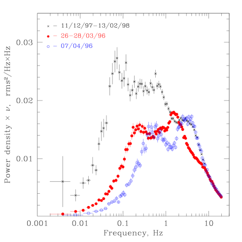
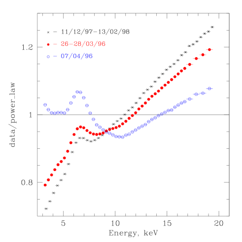
Figure 1: The power density (left) and counts (right) spectra of Cyg X–1 at different epoch. The power density spectra are plotted as frequency $\times$ (power density), i.e. in units of $\rm Hz\times rms^{2}/Hz$. The counts spectra are shown as a ratio to a single slope power law model. The symbols are the same in the left and right panels. The higher characteristic noise frequencies correspond to steeper energy spectra with stronger reflection features.

2 Observations and data analysis

We used the publicly available data of Cyg X–1 observations with the Proportional Counter Array aboard the Rossi X-ray Timing Explorer performed between Feb. 1996 and Feb. 1998 during the low (hard) spectral state of the source. In total our sample contained 26 observations randomly chosen from proposals 10235, 10236, 10238, 20175 and 30157 (Table 1). The energy and power density spectra were averaged for each individual observation. The 4-20 keV flux from Cyg X–1 varied from $\sim 7.2\cdot 10^{-9}$ to $\sim 1.8\cdot 10^{-8}$ erg/sec/cm² which corresponds to luminosity range of $\sim 5.4\cdot 10^{36}-1.3\cdot 10^{37}$ erg/sec assuming a 2.5 kpc distance.

The power spectra were calculated in the 2–16 keV energy band and the $\approx 0.002-32$ Hz frequency range following the standard X–ray timing technique and normalized to units of squared relative rms. The white noise level was corrected for the dead time effects following Vikhlinin et al. (1994) and Zhang et al. (1995).

The energy spectra were extracted from the “Standard Mode 2” data and ARF and RMF were constructed using standard RXTE FTOOLS v.4.2 tasks. We assumed a 0.5% systematic error in the spectral fitting. The “Q6” model was used for the background calculation. We used XSPEC v.10.0 (Arnaud (1996)) for the spectral fitting.

3 Results

Several power density and counts spectra of Cyg X–1 observed at different epoch are shown in Fig.1. The power density is plotted in the units of frequency$\times$power presenting squared fractional rms at a given frequency per decade of frequency. This way of representing the power spectra clearly characterizes the relative contribution of variations at different frequencies to the total observed rms. Most of the power of aperiodic variations below $\sim 30$ Hz is approximately equally divided between two broad, $\Delta\nu/\nu\sim 1$ “humps” separated in frequency by a $\sim$decade (the left panel in Fig.1). The lower frequency “hump” corresponds to what is usually referred to as a band limited noise (e.g. van der Klis (1995)). The second “hump” is sometimes called a “QPO”. Both frequencies are equally important quantitative characteristics of the aperiodic variability – most of the apparently observed variability, indeed, occurs roughly at these two characteristic frequencies (Fig.1). Despite of a factor of $\sim 10-15$ change of the characteristic noise frequencies in our sample, the high frequency part of the power spectrum, above $\sim 8$ Hz, remains unchanged (cf. Belloni & Hasinger (1990)). However, the low and intermediate frequency parts, responsible for the most of the observed variability, change in an approximately self–similar manner which can be described as a logarithmic shift along the frequency axis (Fig.2) (cf. van der Hooft et al. (1996)). This is a manifestation of the fundamental correlation between the break and the QPO frequencies found by Wijnands & van der Klis (1999) and Psaltis et al. (1999) for a broad range of the source types.

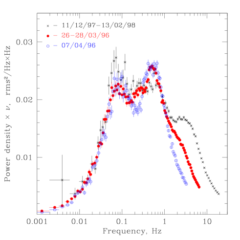
Figure 2: The power density spectra of Cyg X–1 for the same datasets as in Fig.1 but logarithmically shifted along the frequency axis and renormalized to match the spectrum averaged over 11/12/97–13/02/98 (thin black crosses) at low frequencies. The power density spectra are plotted as frequency $\times$ (power density), i.e. in units of $\rm Hz\times rms^{2}/Hz$. The symbols are the same as in Fig.1.

Figure 3: The photon index of the underlying power law plotted vs. reflection scaling factor. See text for discussion of the spectral model.

The counts spectra change in accordance with the change of the noise frequency (cf. left and right panels in Fig.1). The increase of characteristic noise frequency is accompanied by the general steepening of the energy spectrum and an increase of the relative amplitude of the reflection features.

In order to quantify this effect we fit the energy spectra in our sample with a simple model consisting of a power law with a superimposed reflected continuum (pexrav model in XSPEC) and an intrinsically narrow line at 6.4 keV. The binary system inclination was fixed at $i=50\degr$ (Sowers et al. (1998), Done & Zycki (1999); see, however, Gies & Bolton (1986)), the iron abundance was fixed at the solar value of $A_{\rm Fe}=3.3\cdot 10^{-5}$ and the low energy absorption at $N_{\rm H}=6\cdot 10^{21}$ cm^-2. Effects of ionization were not included. In order to approximately include in the model the smearing of the reflection features due to motion in the accretion flow the reflection continuum and line were convolved with a gaussian, which width was a free parameter of the fit. The spectra were fitted in the 4–20 keV energy range. For the spectrum of 07/04/96 (observation 10238–01–04–00) an additional soft component (XSPEC diskbb model) was included in the model. This observation occurred shortly before the soft 1996 state of the source. The energy spectrum had the largest amplitude of reflection and the power spectrum showed the highest noise frequencies (open circles in Figs.1 and 2). The best–fit parameters are listed in Table 1. The accuracy of the absolute values of the best–fit parameters is discussed in the next section.

The model describes all the spectra in our sample with an accuracy better than $\approx 1\%$ and reduced $\chi^{2}_{\rm r}$ in the range 0.5-1.1. The quality of the fit decreases by somewhat with the increase of the best fit value of the reflection scaling factor. The model, however, fails to reproduce the exact shape of the line and, especially, of the edge. Nearly the same pattern of systematic deviations of the data from the model was found for all spectra in the $\sim 6-12$ keV energy range. Inclusion in the model of the effect of ionization and/or account for the exact shape of the relativistic smearing, assuming Keplerian motion in the disk, does not change significantly the pattern of residuals.

We found a fairly good correlation between the photon index of the underlying power law and the reflection scaling factor $R\approx\Omega/2\pi$ roughly characterizing the solid angle subtended by the reflecting media (Fig.3). Other parameters change in an anticipated way indicating that the the spectral model includes the most physically important features. In particular, the width of the Gaussian used to model the smearing of the reflection spectrum and the equivalent width of the 6.4 keV line increase as the reflection scaling factor increases, the equivalent width being roughly proportional to $R$.

Figure 4: The PDS frequency scaling factor plotted vs. reflection scaling factor (top) and photon index of the underlying power law (bottom). The vertical axis on the right hand side of the plots is labeled in units of the PDS break frequency.

In order to relate spectral properties with characteristic noise frequency we fit the power density spectra with a template, allowing logarithmic shift of the template spectrum along the frequency axis and its renormalization. Only the low and intermediate frequency part of the power spectra, up to the second “hump”, was used in the fitting (cf. Fig.2). The best fit values of the two parameter of the fit, the frequency shift and the normalization, were searched for using the $\chi^{2}$ minimization technique. In order to compute the $\chi^{2}$, the template spectrum, logarithmically shifted along the frequency axis, was rebinned to the original frequency bins using linear interpolation . We chose the average power spectrum for observations 10238–01–05–00 and 10238–01–05–000 as a template. The best–fit values of the frequency scaling factor obtained in such a way are listed in Table 1. Fig.4 shows the frequency scaling factor plotted versus reflection amplitude (top) and photon index of the underlying power law (bottom).

The change of the template power spectrum does not affect the correlations shown in Fig.4. More sophisticated spectral models including the effect of ionization and/or the exact shape of the relativistic smearing, assuming Keplerian motion in the disk, change the particular values of the best fit parameter but do not remove the general trends in Figs. 3 and 4. The same is true for a reflection model based on the results of our Monte–Carlo calculations of the reflected spectrum (an isotropic source above an optically thick slab with solar abundance of heavy elements; ionization effects included) in which the equivalent width of the K–$\alpha$ line is linked to the amplitude of the absorption K–edge and of the reflected continuum. More sophisticated spectral models affect mostly the value of the reflection scaling factor, increasing the scatter of the points along the horizontal axis in Fig.3 and in the top panel in Fig.4. The scatter of the values of photon index, on the other hand, almost does not change.

4 Discussion

We found a correlation between the noise frequency and spectral parameters, in particular, the amount of reflection and the slope of the underlying power law. The increase of the noise frequency is accompanied by the steepening of the spectrum of the primary radiation and the increase of the amount of reflection.

The correlation between the spectral parameters – amount of reflection and the slope of the primary emission – is the same as recently found by Zdziarski et al. (1999) for a large sample of Seyfert AGNs and several X–ray binaries. The existence of such a correlation hints at a close relation between the solid angle subtended by the reflecting media and the influx of the soft photons to the Comptonization region. More specifically, it suggests that the reflecting media gives a dominant contribution to the influx of the soft photons to the Comptonization region. The geometry, commonly discussed in application to the low spectral state of X–ray binaries, involves a hot quasi-spherical Comptonization region near the compact object surrounded by an optically thick accretion disk. In such a geometry it is natural to expect that the decrease of the inner radius of the disk would result in an increase of the solid angle, subtended by the reflector (disk), and an increase of the energy flux of the soft photons to the Comptonization region. The correlated behavior of the noise frequency and spectral parameters suggests, that a decrease of the inner radius of the disk leads also to an increase of the noise frequency.

Figure 5: The photon index of the underlying power law plotted vs. reflection scaling factor for both low (solid circles) and high (open circles) spectral states. The low state data are the same as in Fig.3. The high state spectra were fit using the same spectral model as the low state data with addition of a soft multicolor disk component. The particular values of the reflection scaling factor, especially for the soft state, are subject to a number of uncertainties (see discussion in the text and Figs.6, 7).

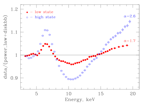
Figure 6: The ratio of the counts spectra to a power law + multicolor blackbody disk emission model for a typical low state spectrum and a soft state spectrum. Each ratio is labeled by the power law photon index used to calculate the ratio.

In the soft state the inner boundary of the optically thick disk is likely to shift closer to the compact object, $R_{\rm d}\sim 3R_{\rm g}$ (cf. $R_{\rm d}\sim 15-100R_{\rm g}$ in the hard state, Done & Zycki (1999), Gilfanov et al. (1998)). Correspondingly, one might expect that the soft state spectra should have stronger reflected component. An accurate estimate of the spectral parameters in the soft state is a complicated task and is beyond the scope of this paper. However, in order to qualitatively check this hypothesis we analyzed a set of RXTE observations of Cyg X–1 in the soft spectral state (May–August 1996). The spectral model was identical to the one used for the analysis of the low state data with addition of a disk component (diskbb model in XSPEC); the energy range was 3–20 keV. We found that the correlation between the slope of the primary emission and the amount of reflection continues smoothly into the soft state (Fig.5), but the best–fit values of the reflection scaling factor are too high and, in particular, considerably exceed unity. However the qualitative conclusion that the amount of reflection increases from the low to the high spectral state is evident from the comparison of typical low and high state spectra (Fig.6). The results of Done & Zycki (1999) and Gierlinski et al. (1999) based on more realistic spectral models also confirm the existence of such a trend – $\Omega/2\pi\sim 0.1$ and $\Omega/2\pi\sim 0.6-0.7$ for the low and the high state respectively.

The spectral model is obviously oversimplified. Therefore the best fit values do not necessarily represent the exact values of the physically meaningful parameters. Particularly subject to the uncertainties due to the choice of the spectral model are the reflection scaling factor $R\sim\Omega/2\pi$ and the equivalent width of the iron line. Our estimates of the reflection scaling factor for the low state are systematically higher than those typically obtained using the more elaborate models $\Omega/2\pi\sim 0.1-0.2$ (e.g. Done & Zycki (1999)). Moreover, the best–fit values of the $R\sim\Omega/2\pi$ for the high spectral state exceed the unity considerably, what is implausible in the usually adopted geometry of the accretion flow. More realistic models, however, impose stringent requirements on the quality and energy range of the data in order to eliminate the degeneracy of the parameters. We therefore chose a model including the most physically important features and satisfactorily describing the data, and on the other hand, having a minimal number of free, especially, mutually dependent parameters. Although the absolute values of the best–fit parameters obtained with such a model should be treated with caution, the model correctly ranks the spectra according to the importance of the reprocessed component. In order to demonstrate this we plotted in Fig.7 the ratio of several counts spectra in the low and the high state with different best–fit values of $R\sim\Omega/2\pi$ to the spectrum with the lowest value of reflection in our sample. The Fig.7 clearly shows that the spectra having higher best-fit values of $R\sim\Omega/2\pi$ have more pronounced reflection signatures – the fluorescent K_α line of iron at $\sim 6-7$ keV and broad smeared iron K-edge at $\sim 7-10$ keV. Similarly we used a simple way of quantifying the characteristic noise frequency in terms of a logarithmic shift of a template spectrum along the frequency axis.

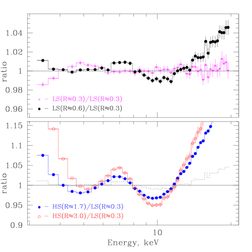
Figure 7: The ratio of the counts spectra in the low (the upper panel) and high (the lower panel) spectral states with different best–fit value of the reflection scaling factor to the low state spectrum with lowest reflection ($R\approx 0.3$). The ratios are multiplied by different power law functions of energy and renormalized. The high and low spectral states are denoted in the legend as “LS” and “HS” respectively. The best–fit values of the reflection scaling factor for different spectra are indicated in the legend. The dotted line in the lower panel shows the ratio for a low state spectrum with $R\approx 0.6$ (the same spectrum as in the upper panel).

Recently, Revnivtsev et al. (1999) applied a frequency resolved spectral analysis to the data of Cyg X–1 observations. They showed that energy spectra corresponding to the shorter time scales ($\la 0.1-1$ sec) exhibit less reflection than that of the longer time scales. Interpretation of the frequency resolved spectra is not straightforward and requires some a priori assumptions. We shall assume below that the different time scale variations occur in geometrically distinct regions of the accretion flow and the spectral shape does not change during a variability cycle on a given time scale. Under these assumptions the frequency resolved spectra can be treated as representing the energy spectra of the events occurring on the different time scales. We reanalyzed the data from Revnivtsev et al. (1999) using the spectral model described in the previous section. We found that the frequency resolved spectra follow the same trend as the averaged energy spectra (Fig.8), thus confirming the existence of an intimate relation between the slope of primary radiation and the amount of reflection. Secondly, energy spectra of the longer time scale ($\sim 0.01-5$ Hz) variations, giving the dominant contribution to the observed rms, are considerably softer and contain more reflection than the averaged energy spectrum. Such behavior hints at the non-uniformity of the conditions in the Comptonization region. Higher frequency variations are associated with a (presumably inner) part of the Comptonization region having a smaller solid angle, subtended by the disk, and a larger ratio of the energy deposited into the electrons to the flux of soft seed photons from the disk.

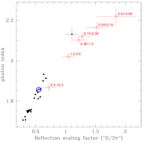
Figure 8: The photon index of the underlying power law plotted vs. the reflection scaling factor for the frequency resolved and average spectra. Solid circles show the best fit parameters for the averaged spectra from our sample (the same data as in Fig.3). The open circles are best fits to the frequency resolved spectra. The numbers near the error bars indicate the frequency range in Hz. The large open circle is a best fit to the spectrum averaged over the datasets used to calculate the frequency resolved spectra.

5 Conclusions

We analyzed a number of RXTE/PCA observations of Cyg X-1 from 1996–1998.

1. We found a tight correlation between characteristic noise frequency and spectral parameters – the slope of primary Comptonized radiation and the amount of reflection in the low spectral state (Fig.3, 4). We argue that the simultaneous increase of the noise frequency, the amount of reflection and the steepening of the spectrum of the Comptonized radiation are caused by a decrease of the inner radius of the optically thick accretion disk.

2. The soft state spectra have larger reflection than the low state spectra and obey the same correlation between the slope of the Comptonized radiation and the amount of reflection (Fig.5).

3. A similar correlation between the slope of the primary radiation and the amount of reflection was found for the frequency resolved spectra. The energy spectra at the lower frequencies (below $\sim$ several Hz), responsible for most of the apparently observed aperiodic variability, are considerably steeper and contain a larger amount of reflection than the spectra of the higher frequencies and, most importantly, than the average spectrum. We suggest that this reflects non-uniformity and/or non-stationarity of the conditions in the Comptonization region.