Weak lensing analysis of MS 1008-1224 with the VLT

Abstract

We present a gravitational lensing analysis of the cluster of galaxies MS 1008-1224 ($z=0.30$), based on very deep observations obtained using the VLT with FORS and ISAAC during the science verification phase.
We reconstructed the projected mass distribution from the B, V, R and I band data using two different algorithms independently. The mass maps are remarkably similar, which confirmed that the PSF correction worked well, thanks to the superb quality of the images.
The J and K band data (ISAAC) were combined with the BVRI (FORS) data to measure the photometric redshifts of galaxies inside the ISAAC field and to constrain the redshift distribution of the lensed sources. This enabled us to scale the gravitational convergence into an accurate mass estimate.
The total mass inferred from weak shear is 2.3 $\times$ 10¹⁴ $h^{-1}$ M_⊙ on large scales (within $\approx 700$ $h^{-1}$ kpc) which is in good agreement with the X-ray mass. The Mass-to-light ratios are also in excellent agreement (319$h$, against 312$h$ from the X-ray). The measured mass profile is well fit by both Navarro, Frenk and White and isothermal sphere with core radius models although the NFW appears to be slightly better.
In the inner regions, the lensing mass is about 2 times higher than the X-ray mass, which supports the long-held view that complex physical processes occuring in the innermost parts of lensing-clusters are responsible for the X-ray/lensing mass discrepancy. We found that the central part of the cluster is composed of two mass peaks whose the center of mass is located 15 arcsecond north of the cD galaxy. This provides an explanation for the 15 arcsecond offset between the cD and the center of the X-ray map already reported elsewhere.
The optical, X-ray and the mass distributions show that MS 1008-1224 is composed of many subsystems which are probably undergoing a merger. It is likely that the gas is not in equilibrium in the innermost regions which vitiates the X-ray mass estimate.
MS 1008-1224 shows a remarkable case of cluster-cluster lensing. The photometric redshifts show an excess of galaxies located 30 arcseconds south-west of the cD galaxy at a redshift of about 0.9. This distant cluster is lensed by MS 1008-1224, which enables the detection of many of its galaxies. Hence, MS 1008-1224 can be viewed as a gravitational telescope facilitating the study of a distant cluster.
These results show that detailed investigations of lensing clusters require very deep imaging with sub-arcsecond seeing in multiple bands (BVRI and JK). Our analysis demonstrates that a thorough investigation of clusters of galaxies and a careful handling of the biases cannot be performed without a dataset which fulfills these requirements. The outstanding capabilities of the VLT at Cerro Paranal make it a unique tool which makes such studies possible.

1 Introduction

The analysis of the distribution of dark matter in clusters of galaxies provides an important insight into the history of structure formation in the Universe. The epoch of formation of clusters and their evolution with redshift are dependent on cosmological parameters and the nature of (dark) matter. For example, the existence of even a few massive clusters at redshift z = 1 would be a strong pointer to a low-$\Omega$ universes.

In order to follow the cosmic history of clusters with look-back time, it is important to have reliable tools at hand to study the nature of matter (the mass, its distribution, the fraction of baryonic and non-baryonic matter etc). Gravitational lensing and bremsstrahlung emission from hot intra-cluster gas are two processes which help us probe these issues. Unfortunately, the results from these two approaches have not yet provided a mutually consistent picture.

Indeed, X-ray mass estimates show discrepancies with weak and strong lensing mass estimates of clusters of galaxies. The origin of the discrepancy is not yet fully understood (see Mellier 1999 for a review). The total mass inferred from lensing exceeds the X-ray mass by a factor of about two for some clusters including well studied clusters like A2218 (Miralda-Escudé & Babul 1995). Investigations of a dozen clusters by Smail et al (1997), Allen (1998) or Lewis et al (1999) have not illuminated the reasons for the discrepancy. In an attempt to solve the problem, Allen (1998) compared cooling flow and non-cooling flow clusters and observed that the former do not show the mass discrepancy. This result suggests that the assumptions regarding the dynamical and thermal state of the hot intra-cluster gas, a key ingredient for the X-ray mass estimate, are not realistic enough to result in a satisfactory model of non-cooling flow (i.e. presumably non-relaxed) clusters of galaxies. This interpretation is confirmed by Böhringer et al (1998) who found an excellent agreement between the X-ray, the strong and the weak lensing analyses of the relaxed cluster A2390. However, Lewis et al (1999) did not find similar trends in their cluster sample. They argue that even some cooling flow clusters show significant discrepancies between X-ray and lensing mass, particularly with strong lensing estimates.

It is likely that this mass discrepancy is the result of several other less-than-valid assumptions. For example, the comparison between X-ray and weak gravitational lensing is done by extrapolating the best fit of the X-ray profile far beyond the region where data are reliable, where uncertainties are obviously significant and the shape of the (assumed) analytical profile used for extrapolation also has a considerable impact on the mass estimate (Lewis et al, 1999; Böhringer et al, 1999).

Lensing mass estimates are not free from bias either. N-body simulations by Cen (1997) and Metzler (1999) show that projection effects of in-falling filaments of matter towards the cluster centre can significantly bias the projected mass density inferred from weak lensing analysis to values higher than from X-ray. The amplitude of the bias seems to range between 10 and 20 per cent, but more generally, projection effects generated by any structures along the line of sight, can overestimate the total mass by about 30 per cent (Reblinsky & Bartelmann 1999). It is therefore important to explore ways which could improve the accuracy of the total mass estimate from lensing inversion algorithms in order to disentangle the systematics from random errors and to separate the contributions of gravitational lensing analyses to the discrepancy from those of the assumptions in the X-ray analyses.

Very deep observations of clusters of galaxies in multiple bands and with subarcsecond seeing can considerably improve the reliability of mass estimates from weak lensing; the depth increases the number density of lensed galaxies thereby improving the resolution of the mass reconstruction; multicolor observations allow estimation of photometric redshifts to be obtain the redshift distribution of background sources; finally, subarcsecond seeing makes for a good determination of object shapes and accurate PSF correction. Rarely are all of these stringent requirements satisfied simultaneously in ground based observations. Fortunately, the recent observations obtained during the Science Verification Programme for the FORS (FOcal Reducer/low dispersion Spectrograph; Appenzeller et al 1998) and the ISAAC (Infrared Spectrometer and Array Camera; Moorwood et al 1999) instruments mounted on the first Very Large Telescope, UT1/ANTU, provide an excellent dataset on the lensing cluster MS 1008-1224. The images obtained at Paranal have a seeing better than 0.7 arcsecond in B, V, R and I bands over a 6 arcminute field of view, as well as on the 2.5 arcminute field covering the central part of the cluster in J and K-bands. The quality and depth of these VLT images are therefore among the best data ever obtained from the ground for weak lensing mass reconstruction of a cluster.

MS 1008-1224 is a galaxy cluster selected from the Einstein Medium Sensitivity Survey (Gioia & Luppino 1994). It is one of the 16 EMSS clusters observed by Le Fèvre et al (1994) in which they found strong lensing features. The cluster is at redshift $z=0.3062$ (Lewis et al, 1999) and is dominated by a cD galaxy. The X-ray luminosity is $L_{X}$(0.3-3.5 keV)=4.5 $\times 10^{44}$ erg.s^-1 (From Lewis et al 1999, with $H_{0}$=100 km s^-1 Mpc^-1 and $q_{0}=0.1$) and its temperature inferred from ASCA observation is $T_{X}=7.29$ keV (Mushotzky & Scharf 1997). According to Lewis et al (1999), the X-ray contours are centered 15 arcseconds to the north of the cD and show a rather circular pattern outward with an extension towards the north.

The paper is organized as follows : Section 2 describes the observations, the data analyses and some optical properties of the VLT images, including the description of some lensed features and magnified distant objects. The mass reconstructions, from weak shear analysis as well as from depletion produced by magnification bias, are presented in Section 3. The results are discussed in Section 4. The main conclusions of the study are summarized in Section 5.

In this paper we have used $H_{0}=100h^{-1}$ kms^-1 Mpc^-1, $\Omega_{0}=0.3$ $\Lambda$ = 0. This corresponds to a typical scale of 176 $h^{-1}$ kpc for 1 arcminute at the redshift of the cluster.

2 Optical properties of the lens MS 1008-1224

The observations were all carried out by the Science Verification Team at ESO. The details of the data processing, from the image acquisition to co-addition and calibration may be found at the ESO web site (see URL in the previous section). Table 1 is a summary of the most important characteristics. The 68 $\times$ 68 field of view of FORS corresponds to a physical size of 1.2$h^{-1}$ Mpc at redshift $z=0.31$. The VLT BVRI data provide a global view of the morphology of MS 1008-1224 and of the field of galaxies around it. The central region of the FORS field is shown in Fig. 1. The gravitational distortion pattern is obvious even on a casual inspection of the VLT images. Together with the X-ray observations of Lewis et al (1999), these high quality multi-band images are well suited for a thorough analysis of the distribution of mass within the cluster.

Source detection and photometry were performed in a standard manner using the latest version of the release 2.1.0 of the SExtractor software (Bertin & Arnoults, 1996) which is publicly available on the TERAPIX web site (http://terapix.iap.fr/sextractor/). The magnitude distributions of galaxies from this field are shown in Figure 5. The stars in the field were identified by their location on the magnitude - half-light radius plot (see Fahlman et al 1994).

2.1 Lensed features

The field shows many lensing features which are good candidates for spectroscopy. Some of the more interesting ones are discussed below. The most obvious central arc is shown in Fig. 1 and Fig. 2. Unfortunately, from its morphology alone, it is not easy to identify the lens configuration. Its shape and its position very close to the cD suggest that this is a radial arc, but its shape on none of the images shows a double structure which would convincingly demonstrate that it is composed of two merging parts of the same source. Alternatively, it could be a tangential arc. In that case, its curvature indicates that the main deflector is to its north. This would imply that the cD is not located at the center of the potential well. Further, an inspection of its image in different bands (Fig. 2) shows that we cannot even exclude that this simply comprises galaxies superimposed along the line of sight.

Some other systems look like typical arcs, like object #2 reported by Le Fèvre et al (1994) and shown on Fig. 1 and Fig. 3. The magnification reveals many structures inside. The irregularities are indications that this is probably a late-type system. Its redshift is lower than 4, since it is visible on the B-image.

We now have spectroscopic observations which show that object #1 in Fig. 1, identified as an arc by Le Fèvre et al (1994), is actually an edge-on spiral within the cluster itself. The $B-\alpha I$ image (Fig. 1) shows its central part is circular and very red, in contrast to its extended and elliptical periphery which is much bluer, as expected for the disk of an edge-on spiral.

Fig. 4 shows a remarkable system which seems to be a magnified dropout candidate. It is located close to a bright cluster galaxy, so it is probably magnified twice, by the cluster as well as by its neighbour on the image. Object #14, located close to object #2 (Fig. 3) also seems to be a very high redshift lensed galaxy.

There are many gravitational pairs in the field. The most obvious one is object #5, with two images of apparently reversed parity. However, the colours of the two objects do not provide conclusive evidence that they are indeed a pair and they could well be unrelated objects. Object #3 also seems to be a gravitational pair. However, we have not found a third image for either of these pairs.

Figure 1: A B-$\alpha$I image of the central parts of the FORS field showing the cluster centre. The square marks the field covered by ISAAC. The coefficient $\alpha$ has been optimized to suppress the central cD and other bright cluster galaxies. This procedure reveals more clearly the very red objects which appear as white features on the image. Conversely, the darkest objects are the bluest galaxies in the field. The arrow at the centre points to the location of (the residual of) the cD. The removal of the bright cluster members makes the background galaxies more visible. The circles indicate some of the interesting features and are labeled with the same numbers as in Le Fèvre et al (1994). Object #1 is the arc candidate reported by Le Fèvre et al which our spectroscopic observation shows is an edge-on galaxy in the cluster. Object 2 is the other arc candidate reported by Le Fèvre et al. Objects #3 and #5 are two pair candidates and object #4 is a radial arc located close to the cD. However, its strong curvature towards the north suggests that it could well be a tangential arc produced by a concentration of matter there. Only a spectroscopic follow-up can establish the possible gravitational nature of these objects.

Figure 2: Zooms of the BVRIJK images of the central arc #4. From left to right: B, V, R, I, J and K image. Its ambiguous shape makes it difficult to decide if it is a radial or a tangential arc. It could be also interacting galaxies or galaxies projected along the same line of sight by accident. This is certainly a system for which spectroscopic data will be useful.

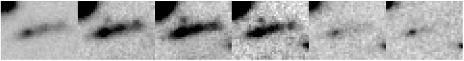
Figure 3: Zooms of the BVRIJK images of the arc #2 reported by Le Fèvre et al (1994). Thanks to the magnification, many structures are visible inside the arc. Note also the small object just above the arc. Note the object #14 at the bottom-right edge of the field. This is likely to be a dropout candidate lensed by the cluster.

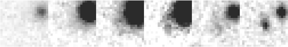
Figure 4: Zooms of the BVRIJK images of the object #13. This is a typical dropout system which is not visible in $B$, so its redshift is probably larger than 4. The system is very close to a cluster galaxy and has probably been magnified twice, by the cluster and by this galaxy as well.

Figure 5: Histograms of the magnitude distribution of the MS 1008-1224 field : B (top left), V (top right), R (middle left), I (middle right), J (bottom left), K (bottom right)

Filter	Exp. Time	Seeing	SB-Lim	Scale
	(sec.)	(arcsec)		(arcsec/pix)
B	4950	0.72	28.25	0.2
V	5400	0.65	27.90	0.2
R	5400	0.64	27.44	0.2
I	4050	0.55	26.37	0.2
J	2880	0.68	-	0.147
K	3600	0.45	-	0.147

Table 1: Summary of the characteristics of the VLT observations of MS 1008-1224 with FORS and ISAAC. These details are taken from the ESO web site. The seeing is the FWHM we measured on the co-added image with SExtractor and IMCAT softwares.

Figure 6: A colour - magnitude (R-I $v/s$ R) plot for the field of MS 1008-1224. The cluster sequence formed by galaxies belonging to MS 1008-1224 is clearly visible as a horizontal strip at R-I = 0.69 $\pm$0.15.

2.2 Distribution of cluster galaxies

The cluster members were identified from the cluster sequence on the color - magnitude plot (R-I $v/s$ R; Fig. 6). The sequence is almost horizontal with these filters. We selected as cluster members all sources having $R-I$ = 0.69 $\pm$ 0.15 and R $<$ 24.

The number density and luminosity density distributions are shown in Fig. 7. The density at a point was calculated by computing the area encompassing a fixed number of nearest sources as well as by counting the number of sources within a certain radius around the point. The distributions shown in Fig. 7 were obtained from counting sources within a fixed radius of 1 arcminute followed by a smoothing of the resulting density field by a Gaussian of 066 arcminute FWHM. There was no significant change when the cluster sequence was extended to a limiting magnitude of R = 27.

Figure 7: Number density contours (top) and R-band luminosity density contours of cluster members in the fields of MS 1008-1224.

The galaxy numbers and the light both extend north from the cD galaxy with a strong concentration around it. One can discern four prominent peaks in the light distribution at (x_pixel, y_pixel) $\equiv$ (1100,1100), corresponding to the location of the cD galaxy, (1040,1400), (1900,1200) and (1280,1520). The number distribution also shows all these peaks which suggests that the enhancement of light is due to a coherent substructure rather than a single bright galaxy. This also indicates that MS 1008-1224 is not yet dynamically relaxed.

2.3 Redshift distribution through the lens

The deep observations of the cluster field in BVRIJK bands with FORS and ISAAC facilitated the determination of the redshift distribution of galaxies with a good amount of accuracy using the photometric redshift technique. For our purpose, we extrapolated the redshift distribution of background sources within the ISAAC field to the rest of the FORS field, where J and K band data are missing, in order to scale the mass obtained from gravitational lensing analysis.

The photometric redshifts were measured using the algorithm described by Pelló et al (1999). It uses photometric data to produce an observed spectral energy distribution (SED) which is then compared to a set of templates comprising a broad range of SEDs of galaxies from the Bruzual & Charlot evolutionary models (Bruzual & Charlot 1993), including a wide range of age and metallicity. The most probable redshifts were then inferred from a $\chi^{2}$ minimization. Since the SED is dependent on many parameters it is important to sample it at many points over as large a wavelength range as possible and to get accurate photometric measurements. The deep FORS and ISAAC images of MS 1008-1224 are therefore ideal for this study. Fig. 8 shows the redshift distributions of galaxies in the ISAAC field; only those galaxies which fit the templates with $\chi^{2}<1$ have been used. The peak at redshift 0.3 corresponding to the cluster is obvious. However, the uncertainties in the photometric redshift estimation have smeared this peak between $z$= 0.27 and $z=$0.40.

Figure 8: Redshift distribution of the galaxies inside the ISAAC field obtained from the BVRIJ and K data. The peak corresponds to the cluster MS 1088-1224. The histogram inside represents the galaxies having very good measurements of photometric redshift, in the magnitude range I=22.5-25.5 corresponding to the galaxies selected for the mass reconstruction in I-band, and with photometric redshift securely larger than the cluster (we choose $z\geq 0.4$).

In the depletion analysis (described later) sources at z $>$ 0.4 formed the background sample while those at z $<$ 0.27 comprised the foreground sample. In the shear analysis, where the sources were selected only by their R-magnitude, the scaling of the mass, including the effect of contamination due to cluster/foreground sources, was done using the redshift distribution of sources in this magnitude range.

3 Gravitational lensing analysis in MS 1008-1224

3.1 Mass reconstruction from weak shear

The weak distortion of background sources produced by gravitational lenses can be used to construct the projected mass distribution of the lens (Schneider, Ehlers & Falco 1992, Kaiser 1992, Fort & Mellier 1994). A considerable amount of effort has gone into making the mass reconstruction more accurate and robust (see Mellier 1999 and references therein).

The remarkable quality of the present data on MS 1008-1224, in terms of seeing, depth and stability of the FORS instrument (I. Appenzeller, private communication) minimize the pitfalls, the critical PSF correction in particular, which tend to limit the production of stable and reliable mass maps. The mass maps for MS 1008-1224 were constructed by two teams working independently, using two different algorithms, to assess the robustness of the result. Both algorithms use the averaged ellipticities of the galaxies to compute an unbiased estimator of the gravitational shear. They differ in the selection of the background galaxies as well as the reconstruction scheme used to obtain the projected mass density.

The mass reconstruction algorithms are rather CPU intensive and we had to run these algorithms over a wide volume of input parameter space to check the stability of our results. The considerable facilities (speed, memory and disk space) of the TERAPIX Data Centre (http://terapix.iap.fr) played an important and extensive part in this study.

Method 1

The IMCAT weak-lensing analysis package has been made publicly available at the URL
http://www.ifa.hawaii.edu/$\sim$kaiser by Kaiser and his collaborators (Kaiser, Squires & Broadhurst 1995, Luppino & Kaiser 1997). The specific version used was the one modified and kindly made available to us by Hoekstra (see Hoekstra et al 1998). A description of the analysis including measurement of the galaxy polarization, correction for the smearing and anisotropy of the PSF and the sizes of galaxies and the expression for the final shear estimate have already been given by Hoekstra et al (1998) and references therein and will not be repeated here.

The maximum probability algorithm of Squires & Kaiser (1996), with K = 20 (number of wave modes) and $\alpha$ = 0.05 (the regularisation parameter), was used to reconstruct the mass distribution from the shear field. Our analysis differs from that of Hoekstra et al only in the weighting of the data at the final stage and is described next.

Error weighting  :  

The contribution of gravitational shear to the polarization of a background source is only a small fraction of its intrinsic polarization. Consequently one has to average the shapes of many (10 – 20) neighboring sources to estimate the gravitational shear at that location. Further, since the noise is much larger than the signal in individual sources their shapes have to be appropriately weighted to obtain meaningful results. Following Hoekstra et al, we estimated the average value of the shear at a location by $\left<\gamma\right>$ = $\Sigma$(W${}_{i}\gamma_{i}$)/$\Sigma$W_i with $\gamma_{i}$ being the shear (intrinsic + gravitational) of individual galaxies and W_i = G_i/$(\delta\gamma_{i})^{2}$ the weight comprising the error on the shear ($\delta\gamma_{i}$) and G_i, a Gaussian factor depending on the distance of the $i$-th galaxy from the location for which the average shear was being calculated. The two components of the average shear thus calculated, which is a function of position, is then to be summed up in the mass reconstruction programme along with appropriate co-efficients to generate the mass map.

While this method works quite well it has the disadvantage in that the error weighting and the Gaussian smoothing are coupled to each other; any reduction in the Gaussian smoothing scale reduces the effectiveness of the all important error weighting of the individual shear values and in the limiting case when the Gaussian smoothing scale includes just one background source there is no error weighting at all. So, apart from $\left<\gamma\right>$, we also calculated the error on it, $\delta\left<\gamma\right>$ = $\Sigma$(G${}_{i}/\delta\gamma_{i})^{2}$ / [$\Sigma$(G${}_{i}/(\delta\gamma_{i})^{2})$ ]². The summations in the mass reconstruction programme were modified to take into account this error on average shear as well.

Source selection  :  

The source detection was done in the R-band using both IMCAT and SExtractor. Only those background (to the cluster) sources which were detected by IMCAT with a significance $>$ 7 and were also detected by SExtractor were used for the lensing analysis. Sources with neighbors closer than 5 pixels (1 arcsecond) were eliminated to reduce the error in the shape estimation. With a series of subsamples spanning a narrow range of $\delta$R = 0.5mag, we detected using Aperture Mass densitometry (described later) a lensing signal for sources in the range 22.5 $<$ R $<$ 26.5. This constituted our master list of 2550 sources for the mass reconstruction analysis. The sources from this master list which were detected in the other 3 bands (B $\equiv$ 2080, V $\equiv$ 2423 and I $\equiv$ 2417 sources) constituted the lensing analysis sample for those bands.

Quality of the mass reconstruction  :  

There are several ways of estimating the quality of the mass reconstruction :
(i) A mass reconstruction after the action of a $curl$ operator on the shear field (effectively replacing $\gamma_{1}$ by $-\gamma_{2}$ and $\gamma_{2}$ by $\gamma_{1}$) must produce a structure-less noise map (Kaiser 1995).
(ii) The boot-strap method
(iii) The location and the intensity of the negative values in the mass reconstruction.

The lensing data set comprising an almost identical sample of sources in each of the 4 bands but obtained under different observing conditions and at different times should provide a good check on the fidelity of the mass reconstruction algorithm. This is particularly true since the gravitational shear signal is such a small fraction of the total noise (intrinsic ellipticity plus measurement) on individual objects.

We also made mass maps using various Gaussian smoothing scales, from 0 (i.e. no smoothing) to 30 arcseconds, to confirm the stability of the reconstruction within an observing band.

Method 2

This method uses the raw IMCAT software from Kaiser’s home page (see previous method) corrected for some minor problems (Erben, private communication). Objects with a significance $>$ 7 and with a raw (smoothed) ellipticity smaller than $0.6$ were used. This resulted in the rejection of all the galaxies with a corrected ellitpicity larger than 1. Such anomalously high values for the corrected ellipticity occurs when the isotropic PSF correction becomes unstable, as in the case of the faintest and/or smallest galaxies. The mass reconstruction was done using the maximum likelihood estimator developed by Bartelmann et al. (1996) with the finite difference scheme described in Appendix B of Van Waerbeke, Bernardeau & Mellier (1999). The mass reconstruction was not regularised and hence the resulting mass maps contain more noise features than in maps obtained from Method 1. However, as pointed out in Van Waerbeke et al (1999) and Van Waerbeke (1999) the advantage of method 2 is that the noise can be described analytically in the weak lensing approximation. We used this property to derive the significance of the offset between the mass peak and the cD galaxy.

Noise properties  :  

The galaxy ellipticities were smoothed with a gaussian window

$$W({{\hbox{$\bf\theta$}}})={1\over\pi\theta_{c}^{2}}\exp\left(-{|{{\hbox{$\bf\theta$}}}|^{2}\over\theta_{c}^{2}}\right).$$ (1)

The noise in the reconstructed mass map is then a 2-D gaussian random field fully specified by the noise correlation function (Van Waerbeke 1999):

$$\langle N({{\hbox{$\bf\theta$}}})N({{\hbox{$\bf\theta$}}}^{\prime})\rangle={\sigma_{\epsilon}^{2}\over 2}{1\over 2\pi\theta_{c}^{2}n_{g}}\exp\left(-{|{{\hbox{$\bf\theta$}}}-{{\hbox{$\bf\theta$}}}^{\prime}|^{2}\over\theta_{c}^{2}}\right).$$ (2)

Figure 9: Mass reconstruction of MS 1008-1224 using the algorithm of Squires & Kaiser (1996) and a Gaussian smoothing of 30 arcseconds. The different maps are : B-band (top-left), V-band (top-right), R-band (bottom-left) and I-band (bottom-right). The mass reconstructions used sources in the range 22.5 $<$ R $<$ 26.5. The contours are of equal magnification ($\kappa$) and the levels are 0, 0.02, 0.04, 0.06, 0.08, $\ldots$ The cross-wire in each panel marks the location of the cD galaxy at pixel (x, y) $\equiv$ (1100, 1100).

3.1.1 Distribution of the dark matter in MS 1008-1224

The mass reconstructions from B, V, R and I data using the first method and a Gaussian smoothing scale of 30 arcseconds are shown in Fig. 9. Figure 10 shows mass reconstructions using the first method with a Gaussian smoothing of 15 arcseconds (B, V, R and I), and for comparison, Figure 11 shows a reconstruction of the I-band image with the second method and a smoothing of $20$ arcseconds. Figure 12 is a high resolution, though noisy, reconstruction in the four bands using the second method. The cross-wire on the maps (Figures 9, 10 and 12) indicates the location of the cD galaxy for reference. Figure 11 shows the I band image in the background.

Mass maps with 30 arcseconds smoothing scale

The reconstructions shown in Fig. 9 are very similar in shape as well as magnitude of the peak ($<$ 5 per cent variation). This certainly speaks for the stability of the mass inversion algorithm and the accuracy of the PSF correction scheme since the PSFs vary from band to band. However, there is still the matter of systematic effects in the mass reconstruction. This is particularly important in the case of algorithms which use an FFT, like the maximum probability algorithm. FFTs often result in correlated noise and artifacts which mimic formally significant (i.e. high signal-to-noise) structures. For example, it is not clear if the low level spur to the north-east is real or an artifact. In particular, we can expect the two large masks on the MS 1008-1224 CCD images (see Fig. 11) to contribute a significant amount of artifacts to mass reconstructions. Eliminating such artifacts will require a deconvolution from the mass map of the effect of the (incomplete) sampling of the data plane. We checked that this mass reconstruction was reliable by comparing it with mass maps obtained using the second method (which does not use an FFT). We found that the results of the two methods matched quite well. It must be noted that the shear inversion algorithms, source selection and the redshift range are all different for the two methods and yet we obtain similar results. There appears to be an offset between the peak of the mass map and the cD galaxy which is consistent with the X-ray observations of Lewis (1999) as well. We have discussed this offset in more detail later.

Figure 10: Mass reconstruction of MS 1008-1224 with a smoothing scale of 15 arcseconds. The maps are : B-band (top-left), V-band (top-right), R-band (mid-left), I-band (mid-right), the intersection of the contours in the above four maps (bottom-right) and the noise map (bottom-right). The contours of convergence ($\kappa$) are 0.0, 0.05, 0.10, 0.15, 0.20, 0.25, 0.30 and 0.35. The negative (dashed) contours of the noise map have the same spacing. The Intersection image delineates features common to all the bands and are therefore most likely to be real. The concentric circles spaced 04 apart on the bottom-left panel are the apertures used for the radial profiles of shear, $zeta$-statistics and mass. The white spot at the centre marks the mass peak in the low resolution map of Fig. 9. The noise map is mostly between $\pm$0.05 and is indicative of the strength of spurious features in the mass maps. The two strong features seen around (300, 1700) and (1500, 1800) correspond to the location of the CCD masks and are a result of the consequent holes in the data. However, the influence of these masks is not significant elsewhere.

Figure 11: Mass distribution of MS 1008-1224 using the algorithm of van Waerbeke et al (1999) and a gaussian smoothing of 20 arcseconds superposed on the R-band image obtained with the FORS on the VLT. This map is to be compared with the I-band map of Fig. 10, although it is more noisy here since the reconstruction is not regularised. Despite the different mass reconstruction algorithm and different source selection (I-band selected with 22.5 $<$ I $<$ 25.5) the agreement is rather good and even better when compared to the intersection image on Fig. 10. The main cluster mass is oriented north-south and offset to the north of the CD. The extensions around the main clump in the intersection image in Fig. 10 seem to coincide with the clumps around the cluster here. The blank regions in the top corners are the CCD masks used to blank out bright stars.

Figure 12: High resolution mass reconstruction of MS 1008-1224 with a smoothing scale of 15 arcseconds using Method 2. The plot at the bottom-left is the average of the reconstructions in the four bands. The noise is reduced by a factor of two in this average map, and it shows the significant elongation of the mass distribution toward the north, as well as a double peak internal structure. The dashed cross shows the position of the cD galaxy which coincides with the south extension of the mass profile.

Noise map

The bottom-right panel of Fig. 10 shows a mass map obtained from the $curl$ of the shear field. In the absence of systematics this is expected to be a featureless image. This is clearly the case over much of the field with the intensity being in the range $\pm$0.05. However, we also see strong positive and negative features at around (300, 1700) and (1500, 1800) which coincides with the location of the CCD masks reported earlier. It is heartening that the influence of the large holes in the data, as a consequence of the masks, does not extend over the rest of the field.

Mass maps with higher resolution

We also constructed mass maps using Gaussian smoothing scales of 0 to 25 arcseconds to (i) explore the mass distribution in more detail, (ii) to confirm that the maps from different scales are consistent with each other and (iii) eventually to probe the inner structure of the cluster. Naturally, the images produced with smaller smoothing scales are noisier. We found that the 15 arcseconds smoothing produced all the details that we could reliably extract and so we have shown these (from B, V, R and I data) in Fig. 10. Considering its noisy nature, we have also reproduced in the same figure an intersection map, comprising the intersection of the contours from all the four bands to delineate the most stable and hence presumably the more genuine structures (as against artifacts). The general features on Fig. 10 are remarkably stable and consistent with the low resolution map on Fig. 9. The inner mass concentration is elongated to the north and consists of 2 peaks. Figure 12 shows maps produced using the second method (which is not regularised) with a smoothing of 15 arcseconds in each of the 4 bands. For convenience the displayed field is restricted to the inner 33$\times$3field. Though noisy, all of them do show the double structure delineated by the reconstruction using the first method. In fact, the co-added map included in the same figure has considerably less noise and clearly shows the double structure. Thus, all the high resolution images show that the central mass distribution of MS 1008-1224 is consists of a double structure. The northern, and the more dominant peak, is coincident with the excess of galaxies seen in Figure 7. The southern peak is well localised on the cD galaxy.

Offset significance

From the noise properties described in Section 3.1 it is possible to obtain the dispersion of the peak mass position due to the random intrinsic ellipticities and the random position of the background galaxies. The best way of measuring the significance of the offset would have been a parametric model for the mass distribution using a parametric bootstrap method to generate a large number of mass reconstructions with different noise realisations and measuring the dispersion of the centroid in these various realisations. Unfortunately such a parametric model is not available and the best that we can do is to consider the mass map reconstructed from the data itself as the mass model. Using the noise model in Section 3.1 we can then generate different noise realisations (since each realisation consists of adding a gaussian correlated random noise to the reconstructed mass map) which simulates mass reconstructions with different realisations of the intrinsic ellipticities and different galaxy positions.

We generated 5000 noise realisations for three different smoothing scales $R_{0}=20",30",44"$ with the I-band image. For each realisation we identified the peak location, and measured the dispersion among the 5000 realisations for the X and Y directions. The results are shown in Figure 13. They show that the offset is most (but not very) significant along the y-axis and in the lowest resolution image which strengthenes the idea that the offset seen at low resolution is not real and is a consequence of 2 mass components in the central regions of MS 1008-1224.

Noise map

The bottom-right panel of Fig. 10 shows a mass map obtained from the $curl$ of the shear field. In the absence of systematics this is expected to be a featureless image. This is clearly the case over much of the field with the intensity being in the range $\pm$0.05. However, we also see strong positive and negative features at around (300, 1700) and (1500, 1800) which coincides with the location of the CCD masks reported earlier (see also the Figure 11 which shows the masks and the induced artefacts in the mass map). It is heartening that the influence of the large holes in the data, as a consequence of the masks, does not extend over the rest of the field.

Figure 13: Parametric bootstrap resampling of the centroid of the mass clump on the I-band image. The left column corresponds to the X-axis offset, and the right column to the Y-axis offset. The position of the cD galaxy is indicated by the vertical dashed lines. Three different scales are represented. The bootstrap were done over 5000 realisations of the noise using the noise model of Van Waerbeke (1999) (see Section 3.1). It shows that the offset is not statistically significant.

A summary of the Features in the mass reconstruction  :  

Having dealt with the principal pitfalls of the mass reconstruction algorithms and the measure procedures, we now proceed to point out the more reliable features in the mass distribution :

• The mass is concentrated in the vicinity of the cD and extends towards the north. This is clearly seen in the high resolution images, particularly in the image formed by the intersection of the mass maps in the 4 bands and in the coadded high resolution image.

• The central concentration when viewed at higher resolution consists of two components. The north-east component appears to be stronger than the south-west peak with which the cD galaxy coincides. However, the significance of the difference in relative strengths is marginal.

• An analysis of the stability of the peaks in the mass reconstruction indicates that while the cD appears to be associated with the southern mass component, its offset from the centre of mass is not highly significant.

• There are other weaker features seen in the high resolution image. For most of them it is not possible to ensure that they are real mass overdensities because they are dangerously close to the edge or the masks of the CCD. One of these, the south-west extension is seen in all the maps, both high and low resolution. The spur extending to the north-east (close to the mask) is also seen in the noise map (Fig. 10) and is therefore likely to be an artifact. We will come back to these later when we compare the mass structures with optical and x-ray data.

3.1.2 Mass Profile from tangential shear

The mass from weak shear, $M_{shear}$, may be obtained from Aperture Mass Densitometry or the $\zeta$-statistics described by Fahlman et al (1994) and Squires & Kaiser (1996). In brief, the average tangential shear in an annulus is a measure of the average density contrast between the annulus and the region interior to it. i.e. The average magnification $\kappa$ ($\equiv\Sigma/\Sigma_{cr}$), the ratio of the surface mass density to the critical surface mass density for lensing, as a function of the radial distance $\theta$ is given by

$$\kappa\left(<\theta_{1}\right) = \kappa\left(\theta_{1}<\theta<\theta_{2}\right)$$ (3)

$$\displaystyle{+\frac{2}{1-\left(\frac{\theta_{1}}{\theta_{2}}\right)^{2}}\int_{\theta_{1}}^{\theta_{2}}\left<\gamma_{t}(\theta)\right>{\rm d}\left(\ln\theta\right)}\ ,$$

where, $\gamma_{t}=-(\gamma_{1}\cos{2\psi}+\gamma_{2}\sin{2\psi})$ is the tangential component of the shear with $\psi$ being the angle between the position vector of the object and the x-axis. One can get an estimate of the error on $\gamma_{t}$ by calculating $\left<\gamma_{r}\right>=-\left<-\gamma_{2}\cos{2\psi}+\gamma_{1}\sin{2\psi}\right>$ which is a measure of the random component of the galaxy shear due to intrinsic ellipticity and observation noise and is expected to be zero around any closed strip. From this we can obtain the average magnification within a series of apertures of radii $\theta_{i}$, $i=1\ldots n$, to derive the radial profile

$$\kappa\left(<\theta_{i}\right) = \kappa\left(\theta_{n}<\theta<\theta_{b}\right)$$ (4)

$$+\frac{2}{1-\left(\frac{\theta_{n}}{\theta_{b}}\right)^{2}}\int_{\theta_{n}}^{\theta_{b}}\left<\gamma_{t}\left(\theta\right)\right>{\rm d}\left(\ln\theta\right)$$

$$+2\int_{\theta_{i}}^{\theta_{n}}\left<\gamma_{t}\left(\theta\right)\right>{\rm d}\left(\ln\theta\right),$$

where, the region $[\theta_{n},\theta_{b}]$ is the boundary annulus which provides the reference density (the first term) in excess of which the interior density values are obtained. Thus this method provides only a lower limit to the lensing mass estimate. It is to be noted that this expression has been cast such that the first term, which cannot be calculated and hence is to be neglected, is the average within the annulus [$\theta_{n},\theta_{b}$] and not the average density interior to $\theta_{b}$. Therefore, the effect of neglecting this term will be quite small if the data extend sufficiently far from the cluster centre.
The mass within an aperture is given by

$$M(<\theta_{i}) = \kappa(<\theta_{i})\ \Sigma_{cr}\cdot\pi\left(\theta_{i}D_{ol}\right)^{2}$$ (5)

$$= \kappa\left(<\theta_{i}\right)\ \theta_{i}^{2}\,\frac{c^{2}}{4G}\left<\frac{D_{ls}}{D_{os}D_{ol}}\right>^{-1}$$

where $D$ is the angular size distance and its subscripts, $l$, $o$, and $s$, refer respectively to the lensing cluster ($z=0.3062$), observer ($z=0$) and the background lensed sources ($z=z_{s}$). As has been explained earlier this high quality dataset allows us to estimate photometric redshifts of sources in the ISAAC field. Assuming that the ISAAC field is representative of the FORS field as a whole we have good photometric redshifts ($\chi^{2}<1$) for 356 objects with 22.5 $<$ R $<$ 26.5 (the lensing analysis range). Of these 302 lie behind the cluster at z $>$ 0.31. We find $\displaystyle{\left<\frac{D_{ls}}{D_{os}D_{ol}}\right>^{-1}}$ = 1.383$\pm$0.031 Gpc which also includes a correction for the dilution of the lensing signal due to foreground objects being in the selected magnitude range. The mass is therefore given by

$$M(<\theta_{i})=6.14\times 10^{14}h^{-1}{\rm M_{\odot}}\ \kappa(<\theta_{i})\ {\theta_{i}^{{}^{\prime}}}^{2},$$ (6)

where $\theta_{i}^{{}^{\prime}}$ is in arc-minute.

The radial profile of the shear, the $\zeta$-statistic, $\zeta=\kappa(<\theta_{1})-\kappa(\theta_{1},\theta_{2})$ , and the mass are shown in Fig. 14. The apertures were centered on the centroid of the mass distribution (x_pixel, y_pixel) $\equiv$ (1175, 1175) in the low resolution mass map. The centre and the apertures, spaced 120 pixel = 04 apart, are marked for reference on the mass map in the bottom-left panel of Fig. 10. The annulus between 32 and 36 radii was used as the boundary annulus to set the zero of the density scale.

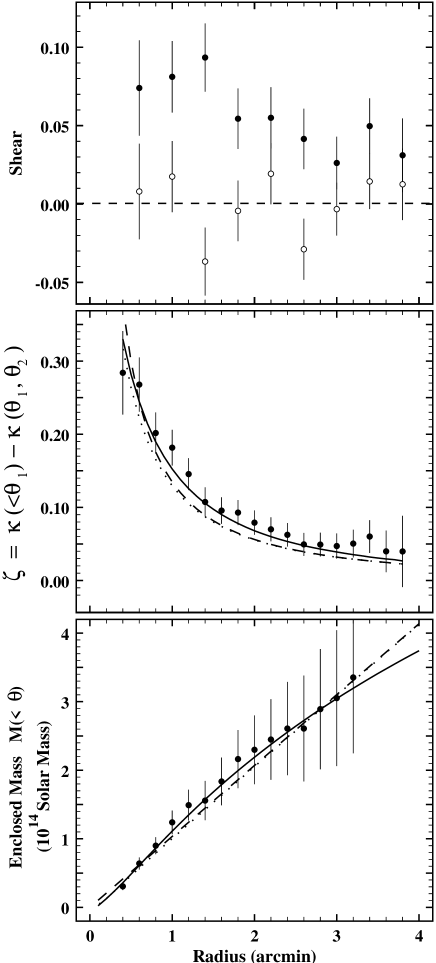
Figure 14: Radial profiles in MS 1008-1224 with the weak lensing analysis of the $R$-selected galaxies. The top panel is the radial tangential shear, centered around the central position given by the joined analysis from weak lensing and depletion (1150,1150). The filled circles are the measured tangential shear. The open circle are the data dat where $\gamma_{1}\rightarrow\gamma_{2}$, and $\gamma_{2}\rightarrow-\gamma_{1}$. The transformated data do have zero amplitude, expected if the tangential shear were produced by a gravitational lensing effect. The bottom panel is the mass enclosed within circular radii. We mass profiles were fitted by an isothermal sphere with a core radius (dashed lines) and an NFW profile (lull lines). The curves show that the NFW profile is slightly better than the isothermal sphere, but the difference is small.

The upper panel of Fig. 14 shows tangential shear (filled circles) within an annulus centered on the radius. Also plotted in the same panel are the values of $\gamma_{r}$ (open circles) which are distributed around zero as expected for a signal due to gravitational lensing. The middle panel shows the $\zeta$-statistics which is the best expression for comparing the data with model fits. The bottom panel shows the mass derived from the shear data. It must be noted that the shear points (top panel) are independent of each other while the points in the lower two panels are not independent; every point makes use of all the shear data exterior to it.

The bars denote $\pm 1\sigma$ error in all the panels. We expect that the quoted errors are actually overestimates because of the linear morphology of the mass and the presence of the two large masks. Since the mass extends to the northern boundary of the field of view, it is likely that we are underestimating the mass of this cluster. We have confirmed that the error estimated for the individual shear values and used in the weighting is appropriate by checking that $\sqrt{\left<\gamma^{2}_{r}\right>/N}\ \simeq(\Sigma^{{}^{N}}_{{}_{1}}1/(\delta\gamma_{r})^{2})^{-1}\ \simeq(\Sigma^{{}^{N}}_{{}_{1}}1/(\delta\gamma_{t})^{2})^{-1}$, where $N$ is the total number of lensed galaxies in the shell.

3.2 Magnification bias and Radial Depletion

As a result of the combined effect of deflection and magnification of light, the number density of galaxies seen through the lensing cluster is modified. In the case of a circular lens, the galaxy count at a radius $\theta$ is

$$N(<m,\theta)=N_{0}(<m)\mu(\theta)^{2.5\alpha-1}\ ,$$ (7)

where $\alpha$ is the intrinsic (without lensing) slope of the galaxy count, $\mu$ the gravitational magnification, and $N_{0}$ the intrinsic galaxy number density (hereafter, the zero-point). Depending on the value of $\alpha$, we may observe an increase or a decrease in the number of galaxies in the central region out to a limiting radius which depends on the shape of the gravitational potential and the redshift distribution of the background sources. This effect produced by the magnification bias has already been observed in some lensing clusters (Broadhurst et al 1995, Fort, Mellier & Dantel-Fort 1996, Taylor et al 1998, Broadhurst 1998). It is particularly obvious in very deep observations as the slope of galaxy counts decreases to values as low as $\alpha\approx 0.2$ at faint levels. The very deep FORS and ISAAC observations of MS 1008-1224 are therefore well suited for studying this effect. In particular, the location of the depleted area provides an independent measurement of the position of the centre of the cluster mass distribution.

3.2.1 Evidence of depletion of lensed sources

As described earlier, we considered as foreground those galaxies which were at $z_{phot}<0.27$ and as background (lensed) those at $z_{phot}>0.4$. We minimized misclassification by considering only those which had a photometric redshift solution with $\chi^{2}<1$. In order to be consistent with the shear analysis samples, we focussed only on the $R[22.5-26.5]$ (method 1) and the $I[22.5-25.5]$ (method 2) samples. We inferred from the FORS data that the slope of the galaxy counts of these two samples were $0.192$ and $0.233$, respectively, which are significantly below 0.4. Therefore, we expected significant depletion with a clear indication of the location of the centre of the mass distribution.

Figure 15: Number density contours of the ISAAC field. The contours show the galaxy number density of the sample $I[22.5-25.5]$ having good photometric redshift. The points are the positions of each galaxy of the samples. The top panel is the foreground sample ($z<0.27$), and the bottom panel the background (lensed) galaxies ($z>0.4$). The distribution of the foreground is, as expected, almost uniform. In contrast, the lensed galaxies are not uniformly distributed and the depletion area is clearly visible. The central contour is centered around the position of the dip. The cross-wire marks the position of the cD. An offset (15 arcseconds west and 20 arcseconds north) is clearly detectable between the maximum depletion location and the cD galaxy, confirming the results obtained previously with the weak shear analysis. This is the first evidence for magnification bias based on sources with known redshift. Note the strong excess of galaxies in the South-West quadrant (quadrant $Q4$), which seems to result from a cluster of galaxies at very large redshift which is lensed by MS 1008-1224.

Figure 15 shows the projected number density of galaxies having good photometric redshifts from BVRIJK data and in the magnitude range $I[22.5-25.5]$. Galaxies at $z>$ 0.4 (background, lensed) are on the right. The control sample of galaxies at $z<$ 0.27 (foreground) are on the left. The difference between the two panels is clear : the foreground distribution is essentially random; in contrast, a strongly depleted area is visible near the centre of the field in the background distribution. This is the first evidence of the magnification bias effect based on a large sample of background galaxies with a known redshift distribution. The cross-wire marks the location of the cD galaxy. The offset of about 20 arcseconds north and 15 arcsecond west between the cD and the depletion is consistent with the previous shear analysis. The depletion and its offset from the cD are also seen in the R-selected sample.

3.2.2 Mass profile from magnification bias

The modification of the radial distribution of galaxy counts due to the magnification bias probes the dark matter distribution. In the weak lensing regime the relation simplifies to :

$$N(<m,\theta) = N_{0}(<m)\mu(\theta)^{2.5\alpha-1}$$ (8)

$$\approx N_{0}(<m)\left[1+2\kappa\left(\theta\right)\right]^{2.5\alpha-1}.$$ (9)

Hence the convergence $\kappa(\theta)$ is

$$\kappa(\theta)={1\over 2}\left[\left(N(\theta)\over N_{0}\right)^{1\over 2.5\alpha-1}-1\right]\ ,$$ (10)

and the total mass inside the radius $\theta$ (in arcminute) is :

$$M(\theta)=4.4\times 10^{14}h^{-1}{\rm M_{\odot}}\left<{D_{ls}\over D_{os}}\right>^{-1}\left({D_{ol}\over{\rm 1Gpc}}\right)\int_{0}^{\theta}\theta\kappa(\theta){\rm d}\theta\ .$$ (11)

The slope of the galaxy counts, $\alpha$, is calculated from the deep FORS data. The depletion curves are also directly provided by the data, either from FORS or from ISAAC, depending on the sample we work on. The quantity $\left<{D_{ls}/D_{os}}\right>^{-1}$ is computed from the redshift distribution shown in Figure 8. So, in principle, we can get the radial mass distribution by merely counting galaxies on the FORS/ISAAC data. However, measurement of the radial depletion is tricky. Since the field of view of ISAAC is smaller than the radial extent of the depletion area, the number density even at the edge of the ISAAC field was not the appropriate value for the zero-point, $N_{0}$.

Even more critical (to the mass estimate) was the significant enhancement of galaxy number density to the south-west direction which enhanced the depth of the radial depletion. This enhancement is clearly visible on the bottom-right quadrant (hereafter the fourth quadrant or Q₄) of the right panel of Figure 15. A visual inspection of the FORS images shows that many faint and distorted galaxies are present between a radius of 250 and 400 pixels from the centre of depletion. This excess is probably produced by galaxy clustering beyond the MS 1008-1224. They are all elongated tangentially with respect to the centre of depletion, which is expected if the distortion is due to gravitational shear. Remarkably, the shape of the number density contours of the smoothed distribution shows similar ellipticity and orientation as individual galaxies, as if they were magnified accordingly.

We compared the photometric redshift distribution of galaxies in Q₄ to those in the other three quadrants (hereafter Q_1-3). The distributions, plotted in Fig. 16, show a significant excess of galaxies at redshift 0.9. Quantitatively, in the magnitude range $I[22.5-25.5]$, the number of galaxies with photometric redshifts in the range $z=0.8-1.1$ is 61 in $Q_{4}$, whereas the three other quadrants together totalize 38 galaxies. So the significance level of the excess is $9.5\sigma$. We therefore conclude that there is a distant cluster of galaxies behind MS 1008 and at $z\approx$ 0.9, which is globally magnified and sheared according to the magnification factor of each individual galaxy. This case of cluster-cluster lensing is the first ever observed so far.

Figure 16: Comparison of the redhsift distribution of the galaxies inside the South-West quadrant ($Q_{4}$) with respect to the others ($Q_{1}+Q_{2}+Q_{3}$). A strong excess of galaxies shows up, at redshift 0.9. This excess is highly significant, more than $6\sigma$ above the average computed from the quadrants $Q_{1,3}$. We conclude that a distant cluster of galaxies lies in this redshift range.

Figure 17: Galaxy number density as function of the radial distance with respect to the centre found from the depletion (1150,1150). All the plots are for galaxies selected in the magnitude range $22.5<I<25.5$. The scale is in pixel units (hence 0.0001 corresponds to 9 gal.arcmin^-2. The dotted curve (top) is the number density found in the FORS field. The plateau at large radius provides the zero-point for the full sample. The other curves are computed from the galaxies inside the ISAAC field, having a good photometric redshift. The full line curve shows the galaxy count form galaxies inside the ISAAC field, including the bottom-right quadrant where a background cluster seems present. The dot-dashed curve show the same plot, where the bottom-right quadrant is now excluded. Finally, he dashed curve (bottom) is the galaxy number density of galaxies with $z_{phot}<0.27$. It is almost flat since the foreground cannot be depleted. The dashed straight lines show the mean number density

This remarkable lensing event has an unfortunate impact, however, on the quantitative analysis of the depletion. This background cluster results in a ”spurious” deepening of the MS 1008-1224 radial depletion profile. Furthermore, since this excess is located at the boundary of the ISAAC field, it is impossible to find out the value of $N_{0}$ (the background density in the absence of a lens, usually obtained from near the edge of the field) from the ISAAC data alone. We need additional information extrapolated from the FORS field as a whole.

We selected galaxies of the FORS field fainter than the brightest cluster members and which are outside the $(I-R)-I$ Color-Magnitude strip defined by cluster members. The contamination by background galaxies and residual cluster galaxies should not be a critical issue and more likely only changes the value of the minimum, not the shape of the depletion curve. Then, we compute the radial galaxy number density of the FORS data within the ISAAC area which excludes the bottom-right quadrant of Figure 8. Fig. 17 shows the growth curves which exclude the forth quadrants of the FORS field as well as the ISAAC subsamples for which we got photometric redshifts. A depletion is visible as well as a flat distribution at large distance, but beyond the ISAAC field and the position of the background cluster at $z\approx 0.9$. The plateau provides the zero points, $N_{0}^{FORS}$, of all $22.5<I<25.5$ galaxies regardless their redshifts. Since the FORS field is composed of foreground galaxies, possibly few cluster members and background galaxies, the depletion of the FORS data can be separated in to components, the foreground (unlensed) galaxies, $Frg$, which include also cluster members, and the background (lensed) galaxies, $N_{0}^{FORS(z>0.4)}$, which is composed of all galaxies with redshift larger than 0.4. :

$$N=N_{0}^{FORS(z>0.4)}\mu^{2.5\alpha-1}+Frg\,$$ (12)

where $\mu$ is the magnification, $\alpha$ the slope of the galaxy counts in this magnitude range. $N_{0}^{FORS(z>0.4)}$ is the zero point of the background galaxies; that is the galaxies of the FORS field having a redshift higher than $z=0.4$. $Frg$ is the density of foreground (unlensed) galaxies. At large distance, the magnification is negligible and we have

$$N_{0}^{FORS}=N_{0}^{FORS(z>0.4)}+Frg$$ (13)

The analysis of the ISAAC field is more complex. Because the success rate of the photometric redshift technique is not 100 per cent of the galaxies having good photometric redshifts $z_{phot}>0.4$, the distribution $N(z>0.4)$ observed from the photometric redshift of the ISAAC field is only an unknown fraction $k$ of the galaxies having a redshift larger than 0.4:

$$N(z>0.4)=k\ N_{0}^{z>0.4}\mu^{2.5\alpha-1}\ ,$$ (14)

where $N_{0}^{z>0.4}$ is the asymptotic value of the galaxy number density of galaxies with redshift larger than 0.4  . At large distance, $N_{0}^{z>0.4}$ is independent of the position, so it must correspond to the background galaxies of the FORS field. Therefore we always have:

$$N_{0}^{z>0.4}=N_{0}^{FORS(z>0.4)}$$ (15)

So the key point is to estimate which fraction $k$ of the background galaxies have a good photometric redshift and which fraction of the FORS sample is at redshift larger than 0.4. This will provide the zero-point of our sample.
The estimation of the foreground (namely, those having $z<0.4$) turns out to be difficult. We cannot use only the sample with photometric redshift $z<0.27$ because we do not know which fraction of the foreground have a good photometric redshift. From the depletion curve of the galaxies with photometric redshift smaller than 0.27, we have a lower limit ($Frg>4.5$ galaxies arcmin${-2}$). However, this does not include galaxies with redshift $0.27<z<0.4$. A crude estimate can be provided by the depletion curve itself. As we can see on Fig 17, the depletion curves of the FORS data is linear below $r=200$ pixels. The intersection with the vertical axis provides a good idea of the background estimate, $Frg\approx 9.0$ galaxies arcmin^-2. Therefore, we have

$$N_{0}^{FORS(z>0.4)}=N_{0}^{z>0.4}=39.6\ {\rm gal.arcmin}^{-2}\ .$$ (16)

We can now estimate the fraction $k$. From Equations (10), (11) and (12) we have

$$k={N(z>0.4)\over N-Frg}\ .$$ (17)

The ratios of the galaxy counts can be explored by comparing the depletion curves of the FORS sample to the depletion curve of the photometric redshift sample inside the ISAAC area, excluding the forth quadrant (see Fig. 17). Since the depletions probe the same parent lensed galaxies, we do expect that the shapes of the curves of the FORS sample and the photometric redshift sample should be similar. In principle, it is possible to infer $k$ from the measurement of the ratio given in Eq. (15) at various points. However, because $k$ depends on the magnification it varies along the radial distance. Furthermore, the depletion curve shows strong fluctuations due to Poisson noise and clustering. In order to minimize these effects, we locally fitted the curve by a straight line and compute and average $k$ inside some radii. Excluding the area $200<r<400$ which shows some residuals of the distant cluster, we find $<k>=0.65_{-0.10}^{+0.10}$. So, the zero-point of the $N(z>0.4)$ sample is $26.3_{-4.5}^{+3.60}$ gal.arcmin^-2.
Using this value we can therefore compute directly $\kappa(r)$. The results are shown on Table 2.

$\theta$	M($\theta,k$=2.42)	M($\theta,k$=2.92)	M($\theta,k$=3.32)	M($\theta,k$=2.00) Simple offset
(arc-min)	$10^{14}h^{-1}{\rm M}_{\odot}$	$10^{14}h^{-1}{\rm M}_{\odot}$	$10^{14}h^{-1}{\rm M}_{\odot}$	$10^{14}h^{-1}{\rm M}_{\odot}$
0.21	1.26	2.70	4.19	0.31
0.50	1.56	3.94	6.03	0.31
0.67	1.56	4.03	7.04	0.31
0.83	1.56	4.03	7.20	0.31
1.00	1.56	4.03	7.20	0.31

Table 2: Mass from the growth curve of galaxy counts of the sample having photometric redshift larger than 0.4. The magnitude range of the galaxies is $22.5<I<25.5$, and the galaxies of the forth quadrant which contains a background cluster have been excluded. The mass is computed for 4 values of $k$. The last one is obtained by simply assuming the depletion curves are similar and are just offset by an amount which gives directly the amount of galaxies at redshift larger than 0.4. For a given value of $k$, the mass increase until we reach the asymptotic value of the zero-point. Due to the poor statistics we cannot provide an accurate growth curve of the mass distribution, which of course should increase beyond one arc-minute.

The table shows that this mass measurement is uncertain and strongly depends on the zero-point. Unfortunately, an accurate calibration is not possible, unless a complete $J$ and $K$ photometric coverage of the total FORS field provides the photometric redshifts of the galaxies with $z>0.4$ located far beyond the cluster centre. Therefore, we cannot expect better results from magnification bias than the gravitational shear ones until then.
The mass from depletion has many sources of errors: Poisson noise statistics on very low numbers and galaxy clustering which seems obvious from the bump observe between $200<r<400$ pixels, whose a fraction comes from a background lensed cluster at redshift $\approx 1$. Unfortunately, the zero-point looks a critical issue. The lower limit of the density of foregrounds seems rather well determined. The intersection of the depletion of the FORS field is a good indication since this curve should have an inflexion because it cannot decrease down to zero. This means that the value of the foreground has probably been minimized. If so, then the density of galaxies with redshift larger than 0.4 could be lowered.
Alternatively, the position of the background galaxy could be estimated by simply offsetting the depletion curve of $z>0.4$ galaxies in order to superimpose to the FORS curve. A crude estimate of the offset, assuming $Frg$ is settled to 1 $10^{-4}$, leads to $k=2.$. As shown in table 2, this strongly lower the total mass.

4 Discussion

It is interesting to compare our results with X-ray and virial analyses. From Fig. 4 of Lewis et al, we see that the mass inside one arc-minute inferred from the X-ray emissivity is $M_{X}(175h^{-1}kpc)\approx 6.\times 10^{13}h^{-1}M_{\odot}$, that is between 1.8 to 2.4 times lower than the shear analysis, $M_{shear}(175h^{-1}kpc)=1.24\pm 0.17\ \times 10^{14}h^{-1}M_{\odot}$. The depletion provides a marginally similar value if $k$ is lower than 2.4, but is difficult to reconcile with the X-ray. The depletion approach is, however, not sufficiently reliable, since we cannot accurately calibrate the zero-point of the photometric redshift sample. It is necessary to have near infrared data over the whole of the FORS field for this purpose.

On larger scale, the agreement is better. $M_{X}$ and $M_{shear}$ monotonically increase and reach $M_{X}=1.82^{+0.34}_{-0.23}\times 10^{14}h^{-1}M_{\odot}$ and $M_{shear}=2.3\pm 0.5\ \times 10^{14}h^{-1}M_{\odot}$ at $r=360h^{-1}kpc$. At that radius, which is the limiting distance to which the X-ray data are reliable, the relative discrepancy is about 20% is within the errors. However, even if we assume that the 20% difference is constant beyond $r=360h^{-1}kpc$, the baryon fraction is not changed significantly with respect to the value quoted by Lewis et al (1999). It only decreases from $f_{b}=0.18$ to $f_{b}=0.14$.

We have compared the mass profile inferred from the shear analysis to three models (see Fig. 14) : a singular isothermal sphere (SIS), an isothermal sphere with core radius and the “universal profile” (Navarro, Frenk & White 1995). A SIS with velocity dispersion of $\sigma=900$ km.sec^-1 fits the data marginally. The agreement is good at large distance, but the discrepancy is important close to the center. A better fit is obtained with an isothermal sphere with a core radius. Using the parameters of the lens configuration (namely the redshift of the lens and the photometric redshift of the lensed galaxies) , the isothermal model with core radius can be expressed as follows :

$$M(x)=1.28\times 10^{14}h^{-1}{\rm M}_{\odot}\left({\sigma_{\infty}\over 1000}\right)^{2}\left({r_{c}\over 1^{\prime}}\right){x^{2}\over\sqrt{1+x^{2}}}\ ,$$ (18)

where $r_{c}$ is expressed in arc-minutes, $x=r/r_{c}$, $M(x)$ the mass inside the radius $x$ and $\sigma_{\infty}$ the three-dimension velocity dispersion at infinity. The best fit predicts $\sigma=900$ km.sec^-1 (as expected from the fit of a SIS) and $r_{c}=45h^{-1}$ kpc. This small value for $r_{c}$ is robust because it is constrained by the change of curvature of the mass profile at small radial distance which imposes an upper limit regardless of the mass at large radius. The presence of strong lensing features also indicates that matter is strongly concentrated at the centre and is consistent with the small core radius. The velocity dispersion is similar within the errors to the galaxy velocity dispersion obtained by Carlberg et al (1996) who measured 1054 km.sec^-1. This confirms that the method they used to measure the velocity dispersion, though it leads to somewhat lower values than previous works, is valid and gives a reliable estimator of the dynamical mass.

The universal profile (NFW) fits the mass profile equally well. The NFW profile may be expressed for this cluster as :

$$M(x)=1.\times 10^{10}h^{-1}{\rm M}_{\odot}\left({r_{s}\over 1^{\prime}}\right)^{3}\delta_{c}\ m(x)$$ (19)

where $x=r/r_{s}$, $m(x)$ is the dimensionless mass profile (Bartelmann 1996) and $\delta_{c}=\rho_{s}/\rho_{c}$, where $\rho_{c}$ is the critical density. Though both the isothermal sphere with core radius and the NFW profiles are within the error bars, the latter fits the data better. In particular on small and intermediate scales, the shape of the radial mass distribution is well reproduced by the NFW. The best fit gives $r_{s}=175h^{-1}$ kpc and $\delta_{c}=3.62\times 10^{4}$.

Fig. 18 shows the radial luminosity profile of the cluster galaxies (selected from the colour-magnitude plot). The luminosity was computed assuming non-evolution models and by using a $K$-correction of elliptical/S0s galaxies for the whole sample. This is a reasonable approximation since the galaxies selected with the color-magnitude diagram are mainly early-type systems and contains the brightest galaxies which contribute most of the luminosity of the cluster. The error bars in Fig. 18 assumed a constant magnitude error of $\delta_{I}=0.1$ regardless the signal-to-noise of the individual galaxies. This conservative estimate makes allowance for the underestimation of the $K$correction for late-type galaxies of the sample. The $K$-corrections have been computed from the most recent Bruzual & Charlot models (Bruzual & Charlot 1993).

The light profile is remarkably linear. Hoesktra et al (1998) found similar results in Cl1358+62. The best fit to the profile gives a slope $a=3.38\pm 0.09\times 10^{11}\ h^{-1}\ L_{{\odot}R}/arcmin$ and $b=-0.032\pm 0.029\times 10^{12}\ h^{-2}L_{{\odot}R}$ (that is, almost zero, as expected). Assuming that the mass-to-light,$M/L$ ratio is constant over the field, this linear profile indicates that an isothermal sphere is an acceptable model for the lens at least up to a radial distance of 700 $h^{-1}$ kpc. However, the profile of the mass-to-light ratio, $M/L(r)$, is more puzzling and does not bear this out.

The integrated $M/L$ over the field is $M/L=319h$, in excellent agreement with the value of the CNOC analysis ($M/L=312h$, Carlberg et al 1996). Fig. 18 shows its radial profile. The lines are the $M/L$ profiles computed from the best fit of the mass distributions (isothermal models or NFW) divided by the best fit of the light distribution (straight line). Clearly, the mass-to-light ratio depends on the radial distance. In the center, it is lower than the average, which expresses the dominating contribution of the cD galaxy to the total luminosity and the fact that this cD is much brighter than normal ellipticals. At large distance, the mass-to-light ratio seems to converge towards a constant value.

The overall shape of $M/L(r)$ is better reproduced by the NFW profile, basically because, if the light distribution increases linearly with radius, the $M/L$ of the NFW profile varies as ${\rm Log}(x)/x$ which shows a maximum at intermediate scale. Therefore, if the $M/L$ is really not constant with radius it would favor the NFW profile against the isothermal sphere. Unfortunately, the error bars are large enough to be consistent with both the profiles. It is worth noting that both profiles underestimate the $M/L$ on intermediate scales. The origin of the discrepancy could be the clustering of sources. In particular, the second cluster at redshift 0.9 certainly increases the amplification and the gravitational shear of galaxies having a redshift larger than one and which are located inside the radius $r<300$ pixels (one arc-minute). Thus, all the galaxies beyond $z=0.9$ are magnified twice. From the depletion point of view, the most distant galaxies are deflected twice, which increases the depth and the angular size of the depleted area. From the gravitational shear point of view, the distant cluster also enhances the distortion that the weak lensing analysis mistakenly interprets as a strong gravitational effect of MS 1008-1224. This could explain why the mass from the weak lensing analysis, and therefore the radial distribution of the mass-to-light ratio shown in Fig. 18, increase rapidly at small radius ($r<300$ pixels) despite a linear increase of the cluster luminosity. A similar effect is also discernable in the depletion which has a very steep growth curve.

The discrepancy between X-ray and lensing mass only appears on small scales. But it is a factor of 2, which is significantly lower than the factor 3.7 obtained by Wu & Fang (1997) from the analysis of strong lensing features. The decrease of the discrepancy with radius seems to be a general trend which has already been reported (Athreya et al 1999, Lewis 1999, see Mellier 1999 and references therein). It must be noted that in most of the studies the comparison has been done between X-ray and strong lensing features and not weak lensing analysis.

Some of the discrepancy observed in MS 1008-1224 can be produced by the distant cluster we have discovered behind it by biasing the mass estimate for MS 1008-1224 towards a higher value. However, such a projection effect, similar to those discussed by Reblinsky and Bartelmann (1999), cannot explain a factor of 2 discrepancy because the distant cluster is only a tiny fraction of the lensed area. It is confined to just one quadrant of the ISAAC field, where, additionally, only background galaxies with redshift higher than 0.9 are magnified twice. The magnitude of its impact on the mass estimate is roughly the ratio

$${1\over 4}\ {\left<{D_{ls}\over D_{os}}\right>^{-1}_{z_{l}=0.9}\over\left<{D_{ls}\over D_{os}}\right>^{-1}_{z_{l}=0.3}}\times{n_{z>0.9}\over n_{z>0.3}}\ ,$$ (20)

where $n_{z>z_{l}}$ is the fraction of lensed galaxies with redshift larger than $z_{l}$ and the factor 1/4 is the fraction of the ISAAC area covered by the cluster. Using photometric redshifts, we estimate that this ratio is about 30 per cent, as predicted by Reblinsky and Bartelmann (1999). In fact, as it is obvious from the mass reconstructions, though we see an extension westward of the mass map at the position of the cluster, no prominent clump of matter is visible and the distortion of the mass maps generated by this second lens seems rather weak.

Figure 18: Top panel:Radial distribution of the luminosity of cluster galaxies located on the cluster sequence on the color-magnitude plot. The profile is remarkably linear. Bottom panel: radial profile of the mass-to-light ratio of MS 1008-1224 inferred from weak lensing and the luminosity of galaxies. The lines represent the best fit Isothermal Sphere with a core radius (dashed) and NFW (solid) profiles.

It is worth noting that apart from this distant cluster, contaminations by other projection effects are not visible at the center, where photometric redshifts provide a good idea of the clustering along the line of sight. The total area covered by ISAAC encompass the region where strong lensing features are visible, where the mass estimate from lensing exceeds the X-ray prediction. We find no evidence that biases like the ones proposed by Cen (1997) or Metzler (1999) are significant in the central region. In contrast, there is some evidence that the innermost regions of MS 1008-1224 is complex, which makes the modeling of the hot gas a difficult task. In particular, there is compelling evidence that the center of mass does not coincide exactly with the cD galxy :

• Lewis et al (1999) reported an offset of the X-ray centroid about 15 arcseconds north of the cD galaxy.

• the mass reconstructions show an offset of 15 arcseconds north and 15 arcseconds west for the low resolution mass maps,

• the depletion area is offseted by 15 arcseconds north and 10 arcseconds west with respect to the cD.

While each of the above results are not highly significant in themselves, the fact that all of them independently point to the offset, and in fact in the same direction strongly suggests that the cD is not at the centroid of the mass distribution. As seen in our high resolution mass reconstruction, it may coincide with the lower subclump. The isoluminosity and number density contours clearly show that the light distribution is clumpy, in particular along the north direction, as in the mass maps. If those clumps overlap along the line of sight they will look like merging system by projection effect and the projected mass density produced by the weak lensing analysis will be centered on the projected centre of mass, if the resolution is too low to separate each component. In fact, the X-ray, the luminosity and the number density contours show elongated and clumpy filaments along the north direction which all indicate that MS 1008-1224 is still experiencing merging processes. If this assumption is valid, then the hot gas is not in equilibrium. The merging process produces shocks and gas flows between clumps, such as those seen in Schindler & Müller’ simulations (1993) or those reported by Kneib et al (1996) and Neumann & Böhringer (1999) in the lensing cluster A2218. Athreya et al (1999) reported similar trends in A370, with remarkable similarity with MS 1008-1224 : a good agreement with X-ray and weak lensing analysis on large scale and a discrepancy of a factor of 2 also in the inner region. Since A370 is clearly composed of merging clumps, Athreya et al also interpret the discrepancy as a result of an oversimplification of the physics of the hot gas. We then suspect that the X-ray analysis oversimplified the dynamical stage of the gas inside MS 1008-1224, producing a wrong estimate of the mass and thus a discrepancy between the X-ray and the weak/strong lensing analysis. This, as suggested earlier by Miralda-Escudé and Babul (1995), easily explains the good agreement on large scale between the weak lensing, the X-ray and also the virial mass (see Lewis et al 1999) and the apparent contradiction between X-ray and strong lensing.

5 Conclusion

Thanks to the deep multicolor subarcsecond images obtained with FORS and ISAAC by the Science Verification Team, it has been possible to map the mass distribution of the lensing cluster MS 1008-1224, to evaluate the reliability of non-parametric reconstruction and to scale the mass carefully. The comparison between the mass map from weak lensing analysis, the X-ray reconstruction and the light distribution from optical data lead to several interesting insights.

• the weak lensing analysis of the FORS data provide stable and reliable mass maps which look similar in B, V, R and I filters. This shows that the PSF correction and the mass reconstruction algorithms work well.

• good BVRIJK photometry allowed for photometric redshift estimation which in turn allowed us to obtain the absolute mass from weak-lensing.

• using the sample with photometric redshift, we discovered a very distant cluster of galaxies located behind MS 1008-1224. This is the first observational evidence of cluster-cluster lensing.

• unfortunately, this lensed cluster partly compromises the use of the depletion curve to estimate the mass of the cluster independent of the weak shear analysis. The slope of the growth curve shows irregularities produced by the excess of galaxies in the lensed clusters. This kind of clustering is is an intrinsic limitation of the practical usefulness of the magnification bias which has already been stressed by Fort et al (1996) and Hoesktra et al (1999).

• On a more optimistic view, MS1008-1224 can be used as a gravitational telescope in order to study the population of a cluster of galaxies at redshift one. Thanks to the magnification, the number density contrast of the distant cluster increases and many more galaxies than the usual fraction visible in such distant clusters can be studied. We have not dwelt on this point since it is far beyond the scope of this work; but a join multicolor and spectroscopic analysis of this cluster could be valuable.

• On large scales, the total mass inferred from weak lensing is in good agreement with the X-ray analysis. In contrast, we still have a considerable discrepancy on small scales. The clumpiness of the light distribution, the elongated shape, the X-ray emissivity and the double peak mass contours are indications that the cluster is still in the throes of a merger. We therefore believe that the X-ray gas is not in equilibrium in the innermost part of the cluster and that this is the principal reason for the mass discrepancy.

In order to go further in the analysis of this cluster we need first a larger coverage of the FORS field in the infrared. This will provide us photometric redshifts of galaxies beyond one arcminute from the cluster center and hence a better estimate of the zero point of the depletion curve. It would be also valuable to get HST images of the center in order to model the innermost regions using strong lensing features. This will provide with a better accuracy the cluster center and can be used to check if the contradiction between the X-ray and the lensing mass can be sorted out by a more accurate lensing model of the cluster center. Photometric redshifts will be particularly helpful since they will provide the redshift of each arc(let). Finally, it would be interesting to get the spectrum of the arc candidate #4. If confirmed as a gravitational arc, then its position and curvature would immediately imply that the center of mass of the cluster is not located on the cD galaxy.

We believe that such a detailed weak-lensing analysis should be carried out on many clusters of galaxies with ground-based optical telescopes. However, the technical requirements for such an investigation are stringent. One must combine very deep observations, subarcsecond images and multicolor photometry, from the B-band up to the infrared K-band. The exceptional combination of FORS and ISAAC on the VLT is the best tool available at present for such a project. It is only after doing similar investigations on a large sample of cluster, that we may be able to obtain a clear understanding of the amount and distribution of dark matter in clusters, understand the reasons behind the the X-ray/lensing mass discrepancy and in general to use weak lensing analysis of clusters as a reliable cosmological tool.

References

- [1] Allen, S.W. 1998. MNRAS 296, 392.
- [2] Appenzeller, I., Fricke, K., Fürtig, W., Gässler, W., Häffner, R., Harke, R., Hess, H.-J., Hummel, W., Jürgens, P., Kudritzki, R.-P., Mantel, K.-H., Meisl, W., Muschielok, B., Nicklas, H., Rupprecht, G., Seifert, W., Stahl, O., Szeifert, T., Tarantik, K. 1998. The messenger 94, 1.
- [3] Athreya, R., Hoekstra, H., Mellier, Y., Cuillandre, J.-C., Narasimha, D. 1999. In “Gravitational Lensing: Recent Progress and Future Goals”. Boston University, July 1999. ASP Conference Series. Eds. T.G. Brainerd and C.S. Kochanek.
- [4] Bartelmann, M. 1996. A&A 313, 697.
- [5] Bartelmann, M., Narayan, R., Seitz, S., Schneider, P. 1996. ApJ 464, 115.
- [6] Bertin, E., Arnouts, S. 1996. A&A 117, 393.
- [7] Böhringer, H., Tanaka, Y., Mushotzky, R.F., Ikebe, Y., Hattori, M. 1998. A&A 334, 789.
- [8] Böhringer, H., Soucail, G., Mellier, Y., Ikebe, Y., Schuecker, P. 1999. A&A submitted.
- [9] Broadhurst, T.J., Taylor, A.N., Peacock, J.A. 1995. ApJ 438, 49.
- [10] Broadhurst, T. 1998. Proceedings of the 19th Texas symposium. J.Paul, T. Montmerle, E. Aubourg Eds.
- [11] Bruzual, G., Charlot, S. 1993. ApJ 405, 538.
- [12] Carlberg, R.G., Yee, H.K.C., Ellington, E., Abraham, R., Gravel, P., Morris, S., Pritchet, C.J. 1996. ApJ 462, 32.
- [13] Cen, R. 1997, ApJ 485, 39.
- [14] Fahlman, G., Kaiser, N., Squires, N., Woods, D. 1994. ApJ 437, 56.
- [15] Fort, B., Mellier, Y. 1994. A&AR 5, 239.
- [16] Fort, B., Mellier, Y., Dantel-Fort, M. 1996. A&A 321, 353.
- [17] Gioia, I., Luppino G. 1994. ApJS 94, 583.
- [18] Hogg, D.W. et al.. 1998. AJ. 115, 1418.
- [19] Hoekstra, H., Franx, M., Kuijken, K., Squires, G. 1998. ApJ 504, 636.
- [20] Kaiser, N. 1992. New Insight into the Universe. V.J. Martínez, M. Portilla, D. Sáez Eds. Springer 1992.
- [21] Kaiser N. 1995. ApJ 439, L1.
- [22] Kaiser, N., Squires, G., Broadhurst, T. 1995. ApJ 449, 460.
- [23] Kneib, J.-P., Mellier, Y., Pelló, R., Miralda-Escudé, J., Le Borgne, J.-F., Böhringer, H., Picat, J.-P. 1996. A&A 303, 27.
- [24] Le Fèvre, O., Hammer, F., Angonin, M.-C., Gioia, I.M., Luppino, G.A. 1994. ApJ 422, L5.
- [25] Lewis, A.D., Ellington, E., Morris, S.L., Carlberg R.G. 1999. ApJ 517,587.
- [26] Luppino, G., Kaiser, N. 1997. ApJ 475, 20.
- [27] Mellier, Y. 1998. ARAA Vol. 37 in press. astro-ph/9812172.
- [28] Metzler, C.A., White, M., Norman, M., Loken, C. 1999. ApJ 520, L9.
- [29] Miralda-Escudé, J., Babul, A. 1995. ApJ 449, 18.
- [30] Moorwood, A., Cuby, J.-G., Ballester, P., Biereichel, P., Brynnel, J., Conzelmann, R., Delabre, B., Devillard, N., Van Disjsseldonk, A., Finger, G., Gemperlein, H., Lidman, C., Herlin, T., Huster, G., Knudstrup, J., Lizon, J.-L., Mehrgan, H., Meyer, M., Nicolini, G., Silber, A., Spyromilio, J., Stegmeier, J. 1999. The Messenger 95, 1.
- [31] Mushotsky, R.F., Scharf, C.A. 1997. ApJ 482, L13.
- [32] Navarro, J.F., Frenck, C.S., White, S.D.M. 1995. MNRAS 275, 720.
- [33] Neumann, D. M., Böhringer, H. 1999. ApJ 512, 630.
- [34] Pelló, R., Kneib, J.-P., Bolzonella, M., Miralles, J.-M.
- [35] Reblinsky, K. Bartelmann, M. 1999. A&A 345, 1. 1999. Preprint astro-ph/9907054.
- [36] Schindler, S., Müller, E. 1993. A&A 272, 137.
- [37] Schneider, P., Ehlers, J., Falco, E.E. 1992. Gravitational Lenses Springer.
- [38] Smail, I., Ellis, R.S., Dressler, A., Couch, W.J., Oemler, A., Sharples, R., Butcher, H. 1997. ApJ 479, 70.
- [39] Squires, G., Kaiser, N. 1996. ApJ 473, 65.
- [40] Taylor, A.N., Dye, S., Broadhurst, T.J., Benítez, N. van Kampen, E. 1998. ApJ 501, 539.
- [41] Van Waerbeke, L. 1999. Prepirnt astro-ph/9909160.
- [42] Van Waerbeke, L., Bernardeau, F., Mellier, Y. 1999. A& A 342, 15.
- [43] Wu, X.-P., Fang, L.Z. 1997. ApJ 483, 62.