Distributed Burning in Type Ia Supernovae: A Statistical Approach

Abstract

We present a statistical model which shows the influence of turbulence on a thermonuclear flame propagating in C+O white dwarf matter. Based on a Monte Carlo description of turbulence, it provides a method for investigating the physics in the so-called distributed burning regime. Using this method we perform numerical simulations of turbulent flames and show that in this particular regime the flamelet model for the turbulent flame velocity loses its validity. In fact, at high turbulent intensities burning in the distributed regime can lead to a deceleration of the turbulent flame and thus induces a competing process to turbulent effects that cause a higher flame speed. It is also shown that in dense C+O matter turbulent heat transport is described adequately by the Peclet number, Pe, rather than by the Reynolds number, which means that flame propagation is decoupled from small-scale turbulence. Finally, at the onset of our results we argue that the available turbulent energy in an exploding C+O white dwarf is probably too low in order to make a deflagration to detonation transition possible.

1 Introduction

The thermonuclear explosion of a C+O Chandrasekhar-mass white dwarf, which is believed to be the underlying process of a type Ia supernova (SN Ia), has been subject to numerous investigations. However, despite the fact that there are different plausible models explaining the history of the explosion (Nomoto et al. (1984); Woosley & Weaver (1986); Müller & Arnett (1986); Livne (1993); Khokhlov 1991a ; Arnett and Livne (1994); Niemeyer & Hillebrandt (1995); Höflich, Khokhlov & Wheeler (1995); Höflich (1995); Wheeler et al. (1995); Höflich & Khokhlov (1996)), many important details still remain unclear. Thermonuclear reactions provide the source of energy which possibly unbinds the white dwarf. Thus, a SN Ia is characterized by the physics of thermonuclear flames that propagate through the star. The physical conditions of this flame vary drastically during the different temporal and spatial stages of this process. A better understanding of these conditions, their interaction with the flame and finally their consequences regarding the explosion itself are still important issues from the theoretical point of view.

Here, we focus on the interaction between thermonuclear burning and turbulence taking place during the burning process. Turbulence is caused by different kinds of instabilities (like shear instabilities or the Rayleigh-Taylor instability) that occur on certain length and time scales (for an overview, see Niemeyer & Woosley (1997)). Rough estimates give a turbulent Reynolds number Re $\approx 10^{14}$ at an integral scale of $L\approx 10^{6}\,$cm (Hillebrandt & Niemeyer (1997)). Consequently, the Kolmogorov scale $l_{\rm k}$, i.e. the scale where microscopic dissipation becomes important, is about $10^{-4}\,$cm. This enormous dynamical range makes a direct representation – at least by means of numerical methods – practically impossible. On the other hand, turbulence is a characteristic feature during the explosion process and it must be considered in any realistic model of a SN Ia. The simultaneous coupling to energy generation due to nuclear reactions leads directly to the physics of turbulent combustion, where a few crucial problems, even for terrestrial conditions, still remain unsolved. These problems include the prescription of the effective turbulent flame speed or the existence of different modes in turbulent combustion along with their physical properties. Global features of turbulent combustion can be systematically classified by a small set of dimensionless parameters. This classification, which already found a wide utilization among the chemical combustion community, can be used in the field of SNe Ia in order to emphasize universality in the physics of turbulent combustion.

In this work we study the properties of turbulent flames in a certain state, the so-called distributed flame regime. The physical characterization of the latter is given by the situation where turbulent motions are fast enough to disturb the flame on microscopic scales. Therefore a distributed flame does locally not look like a laminar flame anymore which is a basic difference to turbulent flames in the flamelet regime. Turbulent burning fronts in an exploding white dwarf are flamelets at high and intermediate densities, but below $\sim 5\times 10^{7}\mbox{g cm}^{-3}$ one cannot expect that the flamelet picture is still valid (Niemeyer & Woosley (1997)).

Until now, in the context of SNe Ia, burning in the distributed regime has only been considered qualitatively. Therefore we wish to present first quantitative results regarding this issue. Furthermore, there are good reasons to believe that this combustion mode plays an important role in the deflagration to detonation transition (DDT), which in turn is a promising model, for empirical and theoretical reasons, for the explosive stage of a SN Ia (e.g. Khokhlov 1991b ; Niemeyer & Woosley (1997); Niemeyer & Kerstein (1997); Khokhlov et al. (1997)).

In order to attempt a representation turbulent dynamics in the distributed flame regime, we use a new model, formulated in one spatial dimension, which nevertheless provides essential features of three dimensional homogeneous turbulence. It consists of a statistical description of turbulent mixing and a deterministic evolution of the underlying microphysics. This method allows a systematical investigation of turbulence phenomena. When it is coupled to a nuclear reaction network, it gives first insights of how the flame structure is affected by turbulence on scales, which have not been resolved in direct numerical simulations. In particular, we investigate the flame properties in cases where the Gibson scale is comparable to the thickness of an undisturbed conductive flame. The Gibson scale $l_{\rm G}$ is defined as the length scale on which the turbulent velocity fluctuations equal the laminar flame velocity. In the case of flames in degenerate white dwarf matter $l_{\rm G}$ becomes comparable to the thickness of the flame only for densities around $2\times 10^{7}\,\mbox{g cm}^{-3}$ and below (Khokhlov et al. (1997); Niemeyer & Woosley (1997)).

The outline of the paper is as follows: first we introduce and describe the statistical method that we use to model turbulence. Then we couple the latter to physically relevant microscopical diffusion processes, such as temperature and viscous diffusion, and to external energy sources coming from nuclear reactions. The resulting method is eventually used to investigate some properties of turbulent flames in the distributed regime, like their effective flame speed. Finally we discuss the relevance of our results to the DDT problem.

2 One-Dimensional Turbulence

Since fundamental aspects of turbulence can be recovered from the knowledge of the statistical moments and correlations of the velocity flow, the statistical approach to turbulence is particulary appealing. Therefore, the history of statistical methods in turbulence theory is rather long. In this context we present a novel model of turbulence (Kerstein (1999)). It is a stochastic method, realized as a Monte Carlo simulation, which allows to compute statistical properties of the flow velocity and of passive scalars in stationary and decaying homogeneous turbulence. One-dimensional turbulence (ODT) represents many aspects of three-dimensional turbulence, but it is formulated in only one spatial dimension. This model provides the temporal evolution of a characteristic transverse velocity profile $u(y,t)$ of the turbulent medium, where $y$ is the spatial location on a finite domain $[0,Y]$ and $t$ is the elapsed time. This is done in a two-fold way: $u(y,t)$ is subject to a molecular diffusion process and to a random sequence of profile rearrangements representing turbulent eddies. Reflecting the typical behavior of turbulence kinematics, the event rate of these profile rearrangements (so-called eddy mappings) is proportional to a locally averaged shear of the velocity profile $u$.
Given the transverse velocity profile at a certain time, $u(y,t)$, the mapping which models the action of an turbulent eddy of size $l$ and at the position $y_{0}$ reads

$$\hat{u}(y,t)=\left\{\begin{array}[]{ll}\!\!\!u(3y-2y_{0},t)&y_{0}\leq y\leq y_{0}+f_{1}l\\ \!\!\!u(-3y+4y_{0}+2l,t)&y_{0}+f_{1}l\leq y\leq y_{0}+f_{2}l\\ \!\!\!u(3y-2y_{0}-2l,t)&y_{0}+f_{2}l\leq y\leq y_{0}+l\end{array}\right.$$ (1)

where it is $f_{1}=1-f_{2}=\text@frac{1}{3}$ and $\hat{u}(y,t)=u(y,t)$ for all $y\notin[y_{0},y_{0}+l]$. This three-valued map represents the typical features of a turbulent vortex, namely rotation and compression. Each random map defines an eddy time scale, $\tau(y_{0},l,t)$, via

$$\ \tau(y_{0},l,t)=\frac{l}{2\,A\,|u_{l}(y_{0},t)-u_{l}(y_{0}+l/2,t)|}\,\,\,.$$ (2)

Here, $u_{l}$ is the boxcar averaged profile of $u$ over a length scale $l$. $A$ is the only model independent and dimensionless parameter which has to be fixed empirically. Vortical kinetic energy is fed by the kinetic energy of the local shear. Thus equation (2) can be interpreted as an energy balance. It then is

$$\frac{1}{2}\,\rho_{0}\,(l\,\tau^{-1})^{2}=\frac{1}{2}\,\rho_{0}\,(2\,A\,|u_{l}(y_{0},t)-u_{l}(y_{0}+l/2,t)|)^{2}\,,$$ (3)

where $\rho_{0}$ is the fluid density. Equation (2) resp. (3) is used to introduce the statistical hypothesis of ODT. It assumes that the occurrence of eddies with size $l$ and location $y_{0}$ (with respective tolerances ${\rm d}l$, ${\rm d}y$) is governed by a Poisson random process with mean event rate

$$\frac{A}{l^{2}\,\tau(y_{0},l,t)}\,{\rm d}y\,{\rm d}l=:\lambda(y_{0},l,t)\,{\rm d}y\,{\rm d}l\,,$$ (4)

where the processes for different values of $y_{0}$ and $l$ are statistically independent. In this context $A$ can be viewed as a factor which scales the event rate $\lambda$. Motivated by the results in Kerstein (1999) we choose $A=0.23$. In addition, the microscopic evolution is modelled by a diffusion process of the kind $u_{t}=\nu\,u_{yy}$, with the kinematic viscosity $\nu$. The temporal evolution of turbulence, stationary or decaying, depends on the choice of boundary conditions for $u$. A decaying turbulent intensity is obtained by periodic boundary conditions, whereas the stationary case is given by the choice of jump periodic boundary conditions: $u(y+Y,t)=u(y)+u_{0},\,\,u_{0}:=u(Y,t=0)$ and $u(y,t=0)$ being strictly monotonic on $[0,Y]$.

The numerical implementation of ODT reproduces many typical features of three-dimensional homogeneous turbulence (Kerstein (1999)). For instance, power spectra of the kinetic energy show the self similar $k^{-5/3}$ power law within the inertial range down to the scale where the transition to dissipation takes place, c.f. Fig. 1. An obvious advantage of this ansatz is the high spatial resolution of turbulence compared with multidimensional numerical models. In combination with the relatively moderate computational effort, ODT appears as a useful tool for performing parameter studies in turbulence theory. On the other hand, ODT does not consider any pressure fluctuations (dynamical or external) in the temporal evolution of the velocity profile $u$. The reason for this artefact is the inherent conservation of kinetic energy in only one spatial velocity component due to equation (3). Note that the pressure gradient term in the Navier-Stokes equations redistributes energy among the different spatial components. No such redistribution is considered here. However, for isobaric flows ODT appears to be an appropriate model of turbulence.

3 Turbulent Flames in Dense C+O Matter

Although the aim of this work is to investigate some properties of turbulent burning in dense C+O matter, we begin this section by recalling some properties of laminar, conductive flames. Since the physics of undisturbed flames inside a white dwarf is relatively well understood, the first reason for it is to verify established results, such as those given in the work of Timmes & Woosley (1992). The other reason is that thermal conduction and viscous diffusion will be employed as the underlying microscopical processes for ODT in order to model turbulent burning fronts in white dwarfs.

The state of unburned matter, i.e. density and nuclear composition, uniquely defines the propagation velocity $s_{\rm l}$ of the conductive flame. Timmes & Woosley (1992) calculated the flame velocities as well as their thickness for various fuel compositions and densities. At lower densities, for $10^{8}\,\mbox{g}\,\mbox{cm}^{-3}\gtrsim\rho\gtrsim 10^{7}\,\mbox{g}\,\mbox{cm}^{-3}$, the speed of the laminar flame decreases rapidly. This behavior is accompanied by a strong increase of the flame thickness $\delta_{\rm l}$, which is essentially the size of the nuclear reactive zone (Timmes & Woosley (1992); Khokhlov et al. (1997)). As already mentioned in the introduction, we are especially interested in densities of the order $\sim(1-3)\times 10^{7}\,\mbox{g}\,\mbox{cm}^{-3}$. Thus, we set up a conductive flame propagating into unburned matter consisting of half ¹²C and half ¹⁶O at densities of $\rho=\,1.3\,\times\,10^{7}\,\mbox{g}\,\mbox{cm}^{-3}$ and of $\rho=\,2.3\,\times\,10^{7}\,\mbox{g}\,\mbox{cm}^{-3}$. This is done by solving the equations for the conservation of mole fractions and enthalpy in planar geometry, viz.

$$\frac{{\rm d}Y_{i}}{{\rm d}t}=\sum_{j,k}-Y_{i}Y_{k}\lambda_{jk}(i)+Y_{i}Y_{k}\lambda_{kj}(i)\,,$$ (5)

$$\frac{{\partial}T}{\partial t}=\frac{1}{\rho c_{\rm p}}\frac{\partial}{\partial x}\left(\sigma\frac{\partial T}{\partial x}\right)-P\frac{\partial}{\partial t}\frac{1}{\rho}+\frac{1}{c_{\rm p}}\dot{S}\,,$$ (6)

$$\dot{S}=N_{\!A}\sum_{i}\frac{{\rm d}Y_{i}}{{\rm d}t}B_{i}\,.$$ (7)

Herein $\dot{S}$ denotes the local specific energy generation rate, $\sigma$ the thermal conductivity and $N_{\!A}$ is Avogadro number and $B_{i}$ is the nuclear binding energy of the nucleus considered. The nuclear reaction network consists of seven species, viz. ⁴He, ¹²C, ¹⁶O, ²⁰Ne, ²⁴Mg, ²⁸Si, and ⁵⁶Ni. Equation (5) already makes use of the fact that the Lewis number, that is the ratio of heat diffusion to mass diffusion, in white dwarf matter is around $10^{7}$ and consequently microscopic transport of the element species can be neglected. Furthermore, in white dwarf matter the laminar flame speed is much smaller than the speed of sound, $s_{\rm l}\,<\,0.001a_{\rm s}$. Therefore pressure does not change significantly across the flame front.

Finally, the typical time scale for free collapse or free expansion of the star can be estimated by (Fowler & Hoyle (1964))

$$\tau_{\rm h}\approx\frac{446}{\bar{\rho}^{1/2}}\,\,\mbox{s}\,.$$ (8)

For a white dwarf of radius $R_{\rm wd}=10^{8}$ cm and of mass $M_{\rm wd}=1.4\,M_{\odot}$, equation (8) gives $\tau_{\rm h}\approx 0.02$ s. Timmes & Woosley (1992) stated that gravitational influence can be safely dropped since the diffusion timescale of the flame, $\tau_{d}\approx\delta^{2}_{\rm l}/D$, where $\delta_{\rm l}$ is the flame thickness and $D$ is the temperature diffusion coefficient, is several orders of magnitude smaller than $\tau_{\rm h}$. However, for very low densities ($\rho\lesssim 10^{7}\,\mbox{g}\,\mbox{cm}^{-3}$) these two timescales can become comparable and a possible expansion of the star could directly affect the laminar flame. To avoid additional complexity we assume in this work that the hydrodynamical timescales is much longer than the relevant timescales of the burning front. Thus we consider the small-scale burning front to be not affected by stellar expansion.

The numerical solution of equations (5) and (6) is given explicitly in time combined with an appropriate equation of state representing ions, black body radiation, electrons and positrons. For $\rho=2.3\times 10^{7}\,\mbox{g}\,\mbox{cm}^{-3}$, Figure 2 shows the propagation of the laminar flame which is indicated by the moving jump in the temperature profile. In the steady state evolution, the flame moves into the unburned matter at a velocity $s_{\rm l}=2.1\times 10^{4}\,\mbox{cm s}^{-1}$. The flame thickness $\delta_{l}$ is characterized by the width of the temperature jump caused by carbon burning. It is $\delta_{\rm l}=1.1$ cm. After ¹²C destruction the burned material has a temperature $3.2\times\,10^{9}$ K and a density of $1.45\times\,10^{7}\,\mbox{g cm}^{-3}$. For these conditions the subsequent oxygen burning has a destruction timescale of $\tau_{\rm des,O}\approx 0.1$ s. That means that as the carbon flame propagates with a steady-state velocity $s_{\rm l}$, oxygen burning ignites at a distance of $2.1\times 10^{3}$ cm behind the flame front. This distance is about ten times larger than our whole computational domain. Consequently, we are not able to track the whole spatial region where nuclear reactions take place that are triggered by carbon burning. The extension of the reactive zone is even larger if one takes burning of heavier elements, such as silicon, into account. Thus, the resolution of the flame with all its reactions up to nuclear statistical equilibrium would require an immense spatial resolution.

However, in our case the fuel consists half of carbon and the destruction of the latter contributes nearly all of the total energy release by the laminar flame. In addition, the speed of the laminar flame is governed by carbon destruction. Therefore it is fair to concentrate only on the latter. We also solved the above equations for a density of $1.3\times 10^{7}\mbox{ g cm}^{-3}$ with the same nuclear composition as before. The resulting flame velocity for this case is $s_{\rm l}=0.85\times 10^{4}\mbox{cm s}^{-1}$, while the flame’s thickness is 3.8 cm. Our results agree well with the ones given in the work of Timmes & Woosley (1992).

As already mentioned in the introduction, the Gibson scale $l_{\rm G}$ can be used to measure the influence of turbulence on a flame. Since it is directly related to the turbulent fluctuation velocity $u^{\prime}$, the Gibson scale depends strongly on the kind of turbulence that is considered. Essential features of turbulence, like structure functions, the temporal evolution of the turbulent intensity and the energy cascade, depend on the absence or presence of certain geometrical (homogeneity, isotropy) and physical (external forces, energy sources, state of the turbulent matter) conditions. On large scales in the interior of a white dwarf, turbulence is mainly caused by the Rayleigh-Taylor instability of the flame which takes place on a length scale of $l_{\rm RT}\approx 10^{6}\,$cm. This instability produces a turbulent energy cascade down to dissipative length scales $l_{\rm k}\approx(10^{-4}-10^{-3})\,$cm (Khokhlov (1995); Niemeyer & Woosley (1997)). On all scales $l_{\rm k}<l\ll l_{\rm RT}$ turbulence is believed to be decoupled from gravitational effects and thus can be described by the Kolmogorov theory. The latter sets the scaling law for $u^{\prime}$ to be $u^{\prime}(l)\sim l^{1/3}$. Inbetween these scale bounds nuclear burning is affected by turbulent motion and different kinds of burning regimes reveal (For an overview, see Niemeyer & Woosley (1997)). Here, we put our emphasis on the special situation where homogeneous, isotropic turbulence interacts with the microscopic structure of the laminar flame, i.e. where $l_{\rm G}$ becomes comparable to $\delta_{\rm l}$. The relation $l_{\rm G}\approx\delta_{\rm l}$ marks the transition into the distributed burning regime, where the smallest turbulent vortices can enter the interior of the laminar flame and can carry away reactive material before it is completely burned (Peters (1986); Niemeyer & Woosley (1997)). Taking into account the small Prandtl numbers in the dense matter of a white dwarf, we can describe this situation by a constraint on the turbulent Karlovitz number. This number is the ratio of the diffusion timescale and the eddy-turnover-time at the smallest length scale of turbulent heat transport. The latter turns out to be the Kolmogorov scale, $l_{\rm k}$, only in case of Pr $\approx 1$. For Prandtl numbers much smaller than one turbulent heat transport is subject to significant diffusion effects already at a scale of $l_{\rm k}\mbox{Pr}^{-3/4}$. Thus we have

$$\mbox{Ka}\equiv\frac{u^{\prime}(l_{\rm k})\,\delta_{\rm l}}{s_{\rm l}\,l_{\rm k}}\,\mbox{Pr}^{1/2}\gtrsim 1\,.$$ (9)

Using Kolmogorov theory an equivalent representation of the latter condition reads

Ka $$= \frac{u^{\prime}(L)\,\delta_{\rm l}}{s_{\rm l}\,L}\,\mbox{Pr}^{1/2}\,\mbox{Re}^{1/2}$$ (10)

$$= \left(\frac{u^{\prime}(L)}{s_{\rm l}}\right)^{2}\,\mbox{Re}^{-1/2}\,\mbox{Pr}^{-1/2}\gtrsim 1\,.$$

There is a simple relation between the Gibson length and the Karlovitz number as follows

$$l_{\rm G}\approx\delta_{\rm l}\,\mbox{Ka}^{-2}\,.$$ (11)

Therefore, $l_{\rm G}<\delta_{\rm l}$ is equivalent to $\mbox{Ka}>1$. The actual value Ka for a given turbulent flame plays an outstanding role in turbulent combustion physics.

We now combine ODT with the structure of a laminar flame to show how certain properties of a nuclear flame in dense degenerate matter of white dwarf depend on the Karlovitz number. The obvious step is to incorporate equation (6) together with a viscous transport evolution for the transversal velocity profile $u(x,t)$. Then turbulent advection is modelled by the random eddy mappings generated by ODT, c.f. equation (1). This system reads as

$$\frac{{\partial}\hat{u}}{\partial t}=\frac{\mathrm{Pr}}{\hat{\rho}\,c_{\rm p}}\frac{\partial}{\partial x}\left(\sigma\frac{\partial(\hat{u})}{\partial x}\right)\,,$$ (12)

$$\frac{{\partial}\hat{T}}{\partial t} = \frac{1}{\hat{\rho}\,c_{\rm p}}\frac{\partial}{\partial x}\left(\sigma\frac{\partial\hat{T}}{\partial x}\right)-P\frac{\partial 1/\hat{\rho}}{\partial t}+\frac{1}{c_{\rm p}}\dot{S}\,,$$

where $\hat{u},\hat{\rho},\hat{T}$ are the rearranged profiles of the velocity, the density and the temperature according to the eddy-mapping, c.f. equation (1).

We choose the amplitude of velocity fluctuations of $u$ to be $\sim 10^{7}$ cm s^-1 at $\sim 10^{6}$ cm, and to obey Kolmogorov scaling. These values are motivated through the expected speed of buoyant unstable hot bubbles of size $L\approx 10^{6}$ cm, which become Rayleigh-Taylor unstable and eventually give the main contribution to turbulent energy on large scales. Having fixed this velocity at a certain lengthscale, we can use Kolmogorov scaling to estimate $u^{\prime}(l)$ on smaller scales $l$. Thus the amplitude of turbulent velocity fluctuations in our model is comparable to the expected small-scale velocity fluctuations within a SN Ia.

However, due to computational limitations we cannot consider $u$ to be the actual fluid velocity of the white dwarf matter. Since its Prandtl number is around Pr $\gtrsim 10^{-5}$, the numerical resolution of both, the viscous and the heat conductive diffusion scale, would cost too much numerical effort even in one spatial dimension. To get out of this dilemma, we use an ’artificial’ Prandtl of $2\times 10^{-2}$ and of $10^{-1}$. This choice underestimates the inertial range of turbulent motions within an exploding Chandrasekhar-mass white dwarf. But we believe that the physics of distributed burning in this kind of matter is decoupled from scales much smaller than $\l_{\rm k}\,\mbox{Pr}^{-3/4}$, because turbulent eddies of sizes well below this limit will be smeared instantly out by temperature diffusion. Therefore, we do not essentially change the flame properties in the distributed burning regime by increasing Pr. Of course, this is only valid for sub-unity Prandtl numbers, otherwise one possibly leaves the distributed regime.

The random velocity field $u$ is generated by stationary ODT, thus $u^{\prime}$ becomes constant in time after an initial transient phase. For our studies we perform simulations where $u^{\prime}$ (at a length scale $l=1$ cm) is equal or larger than a given value $s_{\rm l}$. Then we estimate some flame properties such as the effective turbulent flame speed, $s_{\rm T}$. So far, analytical results do not predict the function $s_{\rm T}(u^{\prime};\mbox{Ka})$ correctly. For instance, experimentally observed bending effects or even complete flame quenching are still mostly unexplained problems (Ronney 1995).

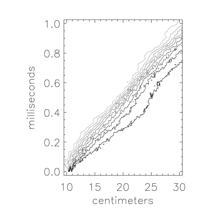
Figure 3: Comparison of a laminar flame (left panel) propagating into C+O matter with a turbulent one (right panel) generated with ODT. The lines represent iso-temperature regions at values from $0.6$ to $3.0\times 10^{9}$ K. The right panel shows data from the numerical realization A2.

An overview of the various numerical models is shown in Table 1. Each realization is uniquely parametrized by its Reynolds, Karlovitz and Prandtl number. To get the turbulent Reynolds numbers, Re $=u^{\prime}(L)\,L/\nu$, we have estimated the integral scale $L$ for each model from the wavenumber $k_{L}$ for which the relevant energy power spectrum $E(k)$ has a maximum. Together with the r.m.s. turbulent velocity and the kinematic viscosity, $\nu={\rm Pr}(\rho c_{\rm p})^{-1}\sigma$, we eventually obtain the Reynolds number Re and the Karlovitz number Ka. An example of a numerical realization is illustrated in Figure 3, where a laminar and a turbulent flame are shown in a space-time diagram.

Table 1 also shows the measured turbulent flame speeds $s_{\rm T}$ as a function of Ka, and Pr. These velocities have been obtained by measuring the slope of the function

$$\Delta(t)=\int c(x,t)\,{\rm d}x\,,$$ (13)

where $c(x,t)$ is the reaction-progress variable defined by (the indices b and u assign the burned and unburned states)

$$c(x,t)=\left(\frac{T(x,t)}{T_{\rm u}}-1\right)\,\frac{T_{\rm u}}{T_{\rm b}-T_{\rm u}}\,.$$ (14)

Thus $s_{\rm T}={\rm d}\Delta(t)/{\rm d}t$ defines the effective flame speed. This value is constant only in the case of laminar flames. However, in the turbulent case it is subject to fluctuations. These estimates enable us to express the dimensionless turbulent flame speed, $U_{\rm T}=s_{\rm T}/s_{\rm l}$, as a function of the dimensionless turbulent fluctuation velocity, $U=u^{\prime}/s_{\rm l}$. We should mention, that we computed the dimensionless turbulent flame speed using the alternative formula

$$U_{\rm T}=\int\rho_{\rm t}\dot{S}_{\rm t}(x)\,{\rm d}x\,(\!\int\rho_{\rm l}(x)\dot{S}_{\rm l}(x)\,{\rm d}x)^{-1}\,,$$ (15)

where $\dot{S}_{\rm t}$ and $\dot{S}_{\rm l}$ denotes the turbulent and laminar profile of the energy generation rate. In fact, the estimated values are in good agreement with the ones obtained through the equation $s_{\rm T}={\rm d}\Delta(t)/{\rm d}t$.

For our studies we vary the r.m.s. turbulent velocity, the Prandtl number and the density while the integral length scale $L$ remains at a constant value.

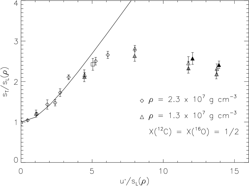
Figure 4: The dimensionless turbulent flame speed as a function of the dimensionless r.m.s. turbulent velocity fluctuations. At high strain rates there is a strong deviation from the flamelet model, which predicts $U_{\rm T}=(1+\beta U^{2})^{1/2}$ (solid curve with $\beta=0.24$), (see for instance Pocheau (1994)). The numerical realization B1 is depicted by a box ($\Box$). The two black triangles give the results from the realizations C41 and C51 having a four-times higher spatial resolution than C4 and C5. The gray triangles represent those speeds obtained from formula (15).

The results are shown in Figure 4. It clearly demonstrates that the turbulent flame speed at high turbulent strain rates, $U\gg 1$, does not follow a law valid in the flamelet regime. At a Karlovitz number greater than one, i.e. in the distributed burning regime, there is a significant deviation from this law: stronger turbulent intensities do not necessarily lead to a faster burning rate. This effect is more pronounced in the low-density case, where higher turbulent velocities even cause a slight deceleration of the flame speed. This result confirms the intuitive picture that fast flames (flames at higher density) are more resistant to distortion through turbulence than the slower ones (flames at lower density).

As already mentioned in this section, the transport of heat is expected to be decoupled from turbulence on scales smaller than $l_{\rm k}\mbox{Pr}^{-3/4}$. This assertion is numerically confirmed in the realization B1, where we significantly decrease the Kolmogorov length scale (using a Prandtl number of $0.02$) while keeping the fluctuation velocity $u^{\prime}(L)$ at a value used in the realization A7 (Pr = 0.1). The estimated turbulent flame speed $s_{\rm T}$ of both models however turns out to be nearly the same, see Figure 4. This behavior suggests that in cases of a small Prandtl number one should use the Peclet number, $\mbox{Pe}=\mbox{Re Pr}$, as the governing parameter for the strength of turbulent flame dynamics.

For clearity, Table 2 gives a summary of all the dimensionless quantities that we have used or mentioned in this section.

4 Discussion

4.1 Burning in the Distributed Regime

The coupling of ODT as a model of homogeneous turbulence to reactive hydrodynamics gives an insight into the physics of distributed burning. First of all the qualitative physical picture of this burning process is revealed: turbulent vortices enter the reaction zone and carry away burning material to the front and to the back of the flame. As a consequence, one observes a completely different behavior than in the flamelet regime, because unlike the latter, the distributed regime changes the local flame velocity (The local flame velocity is the speed at which the flame propagates locally normal to itself.).

A different feature is the existence of localized burning with high burning rates, commonly referred to as a local explosions (Radford & Chan (1995)). Turbulent motion forms regions where hot reaction products are mixed with cold unburned material. These regions have a higher temperature than pure fuel and possess comparably short destruction timescales for carbon. Their eventual re-ignition causes high burning rates, as shown in Figure 5. We find that with higher Karlovitz number more of these events occur and their strength (burning rate) is increased. Terrestrial experiments show the generation of blast waves after the occurrence of local explosions. In some experiments the strongest waves developed even into a detonation (Radford & Chan (1995)). However, laboratory experiments on turbulent flames deal with much higher expansion factors, $\rho_{\rm u}/\rho_{\rm b}$, than those given by flames in white dwarf matter. Thus we expect the effect of blast waves in the context of SNe Ia to be less effective than in typical chemical flames. However, because our model does not consider pressure waves, the whole effect of local explosions on the burning process cannot be presented here and we cannot completely exclude the possibility that blast waves possibly enhance the global burning rate by compression and pre-heating of the surrounding medium. Neglecting such effects in our model possibly means an underestimation of turbulent combustion rate in the distributed regime.

Taking into account the estimates on the turbulent flame speed of Table 1 we obtain a relatively good agreement with experimental data presented by Abdel–Gayed et al. (1987), henceforth AG97. Their work contains about 1650 experimental results on turbulent flame velocities at various strain rates $U=u^{\prime}/s_{\rm l}$, fuels and equivalence ratios. Their results were obtained under conditions far from those in an exploding Chandrasekhar-mass white dwarf, but it is worth to verify if certain physical statements, like the function $U_{\rm T}({\rm Ka};{\rm Re})$, appear to show universality. These experimental results and earlier work (Abdel-Gayed & Bradley (1985)) present two important phenomena. First, for a fixed Reynolds number, $U_{\rm T}$ is not a strong monotonic function of the strain rate $U$. Rather, it reaches a maximum at a certain turbulent intensity and eventually saturates or even decreases for higher values of the strain rate (bending effect). As a second feature, there is flame extinction at a Karlovitz number Ka $\gtrsim 7$ for Reynolds numbers Re $>10^{2}$. Figure 6 shows several experimemtal values of the function $U_{\rm T}$ taken from the work of AG87. These values correspond to the same sample of ratios $u^{\prime}/s_{\rm l}$ we use in our numerical caluclations.

Our numerical results do show the bending effect for high strain rates which is in agreement with laboratory experiments. However, they do not show complete flame quenching, i.e. a situation where fuel is not consumed anymore. This is not surprising because the basic laws of thermodynamics prevent a turbulent (or laminar) flame from complete quenching. The first law of thermodynamics states that the reactive mixture must eventually reach the adiabatic flame temperature. The second law demands that heat must be transported from the burned to the unburned regions. Therefore, there is no way to prevent consumption of unburned material in a system without possible heat losses. And clearly, unlike under laboratory conditions, the flame in an exploding white dwarf is not subject to significant heat losses.

The comparison with our results shows that the flame speeds presented here are lower than those in AG87. We think that one reason for this discrepancy is the different value of the Lewis number in our work and in the data of AG87. It is known that high Lewis number flames are more sensitive to strain than flames with a low value of Le. In fact, analytical results on planar laminar flames show that the flame speed decreases when a velocity field with strain, i.e. a non-vanishing gradient of this velocity field, is invoked parallel to the flame surface. One finds that at higher Lewis numbers the decrease of the flame speed is stronger (Tromans (1981)). Therefore we expect thermonuclear flames in C+O matter to be more sensitive on strain effects, because of their Lewis numbers of aprrox. $10^{7}$. Another source of this deviation could be the already aforementioned difference in the expansion factors between laboratory and white dwarf combustion.

Thermonuclear flames in the distributed regime thus experience a two-fold effect through turbulence: One is the acceleration due to an enhancement of the heat transport produced by small-scale turbulence. The other is a slowing-down due to additional turbulent strain, which can be measured by the Karlovitz number. However, we have to stress that we do not have revealed the actual physical mechanism responsible for the deceleration. This is the task of future work.

4.2 Implications for a Deflagration to Detonation Transition

As already stated by many authors, a delayed detonation within the explosion of a Chandrasekhar-mass white dwarf is a reasonable model. It is a good fit to experimental constraints for element abundances obtained from observed spectra. In addition, although it is almost clear that after ignition the burning process evolves as a deflagration, there is no fundamental physical objection why a transition to detonation in the subsequent stages of the explosion should be impossible. Therefore, DDT models should be taken into account in supernova theory. In the context of this work, we discuss the possibility of distributed burning leading to a detonation.

Based on the Zeldovich gradient mechanism, Khokhlov et al. (1997) calculated the minimum size, $L_{c}$, of a region where fuel and ashes are mixed and out of which a stable detonation wave can emerge. In their model the formation of this region is caused by turbulent mixing, but it is not obvious how this process is realized. They proposed that global expansion of the star along with the following density drop quenches the deflagration flame, whereas the Rayleigh-Taylor instability still takes place on scales of $10^{6}$–$10^{8}$ cm. Before the star recompresses again, fuel and ashes are mixed and turbulence eventually produces a complete mixed region of size of the order of $L_{c}$. Thus, pulsation may lead to a DDT.

Apart from considering pulsations of the star, it is worth asking whether burning in the distributed regime alone can lead to a DDT. Niemeyer & Woosley (1997) advocated this burning mode as a favorite model for DDT. Basically, they proposed that if turbulent burning is able to form a region of uncompletely burned material with a certain temperature gradient, then a carbon detonation can occur when two presumtions are fulfilled. First, the aforementioned region must have at least a size of the critical radius necessary for a detonation (These critical radii could be calculated explicitly for different densities and nuclear compositions, see Niemeyer & Woosley 1997.). Second, the temperature gradient must be shallow enough in order to allow a sonic phase velocity of nuclear burning. For instance, consider a mixed region consisting of half carbon and oxygen at a density of $3\times 10^{7}\mbox{g cm}^{-3}$ and having a maximum temperature of $T_{\rm max}=2\times 10^{9}$ K. It then follows that this region must have a size of at least $L_{c}\sim 50$ m. Furthermore, temperature differences within it should nott exceed $\sim 10^{5}$ K. Then a stable detonation wave can form.

Both approaches have in common that they require a rather shallow temperature gradient over a region with a sufficient amount of carbon. Until now, it has not been demonstrated how turbulence can achieve or lead to such a high level of temperature homogeneity.

In this context it is interesting to know the maximum length scale, $l_{\rm max}$, where distributed burning in a white dwarf can occur. A lower bound of this scale is given by the size of those eddies whose turnover time equals a typical turbulent burning timescale $\tau_{\rm nuc}$. That is

$$l_{\rm max}/u^{\prime}(l_{\rm max})=\tau_{\rm nuc}\,.$$ (16)

In the case of laminar flames $\tau_{\rm nuc}$ is just the diffusion timescale $\tau_{\rm l}\approx\delta_{\rm l}/s_{\rm l}\approx 0.7\times 10^{-4}$ s. But what is the value $\tau_{\rm nuc}$ in the presence of turbulence? We argue that even in the turbulent case the choice of $\tau_{\rm l}$ as the typical burning timescale is natural. To justify this assumption, we compute the spatial distribution of destruction timescales across the flame. In general, this distribution is characterized by a minimum value $\tau^{*}_{\rm nuc}$. It corresponds to the location of the maximum energy generation within the flame. In our numerical models, we find that $\tau^{*}_{\rm nuc}$ is independent of the turbulent intensity, i.e. its value is the same for the laminar case and for the distributed regime. In fact, $\tau^{*}_{\rm nuc}$ equals $\tau_{\rm l}$. Then equation (16) leads to the useful expression

$$l_{\rm max}\approx\delta_{\rm l}\,\mbox{Ka}\,.$$ (17)

This number can be viewed as the size of the distributed flame, i.e. an estimate on the size of the interface that seperates burned and unburned material. However, there are reasons to believe that in reality $l_{\rm max}$ exceeds the value given by equation (17). This is because there are turbulent vortices with bigger size than $l_{\rm max}$ that can enter the flame and transport burning material with longer burning times than $\tau_{\rm nuc}$. Hence, we do justice to these considerations and set the effective value of $l_{\rm max}$ to

$$l_{\rm max}\approx\alpha\,\delta_{\rm l}\,\mbox{Ka}\,,$$ (18)

with $\alpha>1$. The actual value of $\alpha$ however, i.e. the ability of turbulence to stretch out the flame brush, has to be estimated by more rigorous and quantitive considerations, see Lisewski et al. (1999).

If $l_{\rm max}$ itself reached the critical size $L_{c}$ required for a detonation, then burning in the distributed regime would become more of a promising model for DDT. But still it would not be clear if present temperature fluctuations would be small enough to allow this transition to happen. Thus the equality of $l_{\rm max}$ and $L_{c}$ is only a necessary condition for a DDT. At a density of $2.3\times 10^{7}\mbox{g cm}^{-3}$, Khokhlov et al. (1997) obtain $L_{c}\approx 10^{4}$ cm. Now the expected turbulent velocities at an integral scale of $L=10^{6}$ cm are $u^{\prime}\sim\sqrt{g_{\rm eff}L}\sim 10^{7}\mbox{cm s}^{-1}$, where $g_{\rm eff}\sim 10^{8}\mbox{cm s}^{-2}$ is the effective gravitational acceleration. Hence, at densities $\rho\gtrsim 2\times 10^{7}\mbox{g cm}^{-3}$ the corresponding Karlovitz numbers are only around Ka $\approx 10$. According to equation (17) a very high Karlovitz number Ka $\approx 10^{4}$ is required to obtain equality of $l_{\rm max}$ and $L_{c}$. Consequently, the enhancement-factor $\alpha$ in equation (18) would have to be of the order of $10^{3}$. This means that the ashes-fuel interface has to be extended much more in size than given by equation (17).
Also at a density of $10^{7}\mbox{g cm}^{-3}$, where $s_{\rm l}=4.7\times 10^{3}\mbox{cm s}^{-1}$ and $\delta_{\rm l}=4.2$ cm (Timmes & Woosley 1992), the value of $\alpha$ has still to be around $10^{3}$ in order to enable a direct DDT.

Furthermore, the process of a DDT demands, that the mixing timescale, $\tau_{\rm mix}$, which can be regarded as the time it takes turbulence to form a complete mixed region of size $L_{c}$, must be smaller than a typical burning timescale, $\tau_{\rm nuc}$, of the mixed turbulent matter. But in order to avoid quenching by expansion, $\tau_{\rm nuc}$ in turn must be smaller than the hydrodynamical time of the star, $\tau_{\rm h}$, c.f. equation (8). These conditions read as $\tau_{\rm mix}\,<\tau_{\rm nuc}<\,\tau_{\rm h}$, or as

$$\frac{L_{c}}{u^{\prime}(L_{c})}<\tau_{\rm nuc}(l_{\rm max}=L_{c})<\frac{446}{\bar{\rho}^{1/2}}\,.$$ (19)

For $\rho=2\times 10^{7}\mbox{g cm}^{-3}$, we have $\tau_{\rm mix}\approx 5$ ms while the hydrodynamic time is $\tau_{\rm h}=0.02$ s. Here now the question arises whether turbulence can form such a region whose burning time is smaller than $\tau_{\rm h}$. This problem is adressed to forthcoming work, where we study – by using ODT – the burning times on different lengthscales within the distributed flame. However, until we do not have a better understanding of the large scale structure (lenght-scales of $\gtrsim L_{c}$) of flames in the distributed regime, the preliminary result from equation (17) suggests that Karlovitz numbers in white dwarf C+O matter at densities around $10^{7}\mbox{g cm}^{-3}$ are too small to form a region of critical size necessary for a DDT.

5 Conclusions

The aim of this work was to investigate the physics of distributed burning in an exploding white dwarf of chandrasekhar mass. With ODT as a new model for homegeneous, isotropic turbulence we are able to study the effective turbulent flame speeds resulting from this kind of burning in dense C+O matter. Our results show that in this regime the local properties of the thermonuclear flame are readily changed: the flame cannot be represented by the flamelet model anymore and moreover, higher turbulent intensities in general can lead to a lower local flame speed. This behaviour has already been observed in laboratory experiments and is introduced the first time in the context of nuclear explosions in type Ia SNe. We have also found that, in cases where the Gibson length $l_{\rm G}$ is smaller than $\delta_{\rm l}$ and where the Prandtl number is much smaller than one, turbulent burning decouples from turbulent scales smaller than $l_{\rm k}\mbox{Pr}^{-3/4}$. This suggests that the appropriate parameter for turbulent heat transport inside a white dwarf is given by the Peclet number instead of the Reynolds number. Because of the small ratio of viscous momentum to diffusive heat transport the former is by several orders of magnitude smaller than the Reynolds number: $\mbox{Pe}=\mbox{Pr Re}$.

In addition, first quantitative considerations demand that a turbulence-induced deflagration to detonation transition can only happen deep in the distributed burning regime, i.e. at Karlovitz numbers larger than $10^{3}$. However, our estimates for the turbulent velocity at the integral scale in an exploding white dwarf give values of Ka that are too small (at least by a factor of $10^{3}$) in order to make a direct DDT probable.

Finally, it is wortwhile to remark that we have completely left out questions about the influence of the turbulent spectrum on this issue. We have only shown that a DDT is unlikely, when Kolmogorov theory of turbulence is considered. Niemeyer & Kerstein (1997) proposed that turbulence in an exploding white dwarf is dominated by a potential energy cascade instead of Kolmogorov’s kinetic energy cascade. This domination leads to different scaling properties (Bolgiano-Obhukov scaling) of the turbulent velocity. As a consequence, higher turbulent velocities are necessary for the transition to distributed burning. Furthermore, Niemeyer & Woosley give the speed of the turbulent fluctuations, $v_{\rm RT}\approx 0.5\sqrt{g_{\rm eff}L}\approx u^{\prime}(L)$, which may not be the upper limit for turbulent velocities at the largest turbulent scale. It is based on the original idea of Kerstein (1996), that the turbulent flame velocity, $s_{\rm T}$ is increased by local expansion caused by thermonuclear reactions (active turbulent combustion). At the largest length scale, $L$, and at a certain temporal stage of the burning process, the speed of the flame may exceed $v_{\rm RT}$. Because the relation $u^{\prime}(L)\approx s_{\rm T}$ still holds at this point, a significant enhancement of turbulent velocity fluctuations may occur. But it is unclear, if the growth rate, $\dot{s}_{\rm T}/s_{\rm T}$, is high enough to realize this enhancement within a hydrodynamical time $\tau_{\rm h}$.
These arguments favour a DDT, because their effect is an increase of the turbulent fluctuations on lengths comparable to $L_{c}$. However, both arguments are rather speculative, because they have not been confirmed numerically, analytically or experimentally in the context of SNe Ia yet.

This work was supported by the Deutsche Forschungsgemeinschaft and the Deutscher Akademischer Austauschdienst. AML kindly acknowledges partial support by the NSF grants INT-9726315 and AST-3731569. Support from the Office of Basic Energy Sciences, U.S. Department of Energy, is also acknowledged (ARK).

Table 1: Realized models of turbulent flames. X(¹²C) = X(¹⁶O) $=\text@frac{1}{2}$, $\rho=2.3\times 10^{7}\,\mbox{\rm g cm}^{-3}$ (A1 – A9, B1), $\rho=1.3\times 10^{7}\,\mbox{\rm g cm}^{-3}$ (C1 – C5, C41, C51).

Model	Reynolds Number	Karlovitz Number	Prandtl Number	Flame Speed
	Re	Ka	Pr	$s_{\rm T}$ [$\times 10^{4}$ cm s-1]
A1	114	0.06	0.1	$2.15$
A2	270	0.23	0.1	$2.4$
A3	452	0.51	0.1	$2.7$
A4	598	0.78	0.1	$3.1$
A5	673	0.92	0.1	$3.4$
A6	820	1.24	0.1	$4.2$
A7	1285	2.43	0.1	$5.0$
A8	1493	3.05	0.1	$5.3$
B1	6182	2.29	0.02	$4.9$
C1	28	0.68	0.1	$1.0$
C2	119	5.80	0.1	$1.8$
C3	212	13.9	0.1	$2.4$
C4	314	25.7	0.1	$2.1$
C41	323	25.3	0.1	$2.2$
C5	366	32.4	0.1	$1.9$
C51	371	32.2	0.1	$2.0$

Table 2: Summary of some important dimensionless parameters.

Symbol	Name	Mathematical definition	Physical description
Re	Reynolds number	$\displaystyle{\frac{u^{\prime}(L)\,L}{\nu}}$	$\displaystyle{\frac{\mbox{integral scale turbulent diffusivity}}{\mbox{viscous diffusivity}}}$
Pr	Prandtl number	$\displaystyle{\frac{\rho c_{\rm p}\nu}{\sigma}}$	$\displaystyle{\frac{\mbox{viscous diffusivity}}{\mbox{heat diffusivity}}}$
Pe	Peclet number	Re Pr	$\displaystyle{\frac{\mbox{integral scale turbulent diffusivity}}{\mbox{heat diffusivity}}}$
Ka	Karlovitz number	$\displaystyle{\frac{u^{\prime}(l_{\rm k})\,\delta_{l}}{s_{\rm l}l_{\rm k}}\mbox{{\rm Pr}}^{1/2}}$	$\displaystyle{\frac{\mbox{heat diffusion timescale}}{\mbox{smallest turbulent heat transport timescale}}}$
Le	Lewis number	$\displaystyle{\frac{\sigma}{\rho c_{\rm p}D_{\rm m}}}$	$\displaystyle{\frac{\mbox{heat diffusivity}}{\mbox{mass diffusivity}}}\,\,$

Figure 1: An energy power spectrum generated by stationary ODT ($\diamond$). Up to a constant factor the power spectrum is the Fourier transform of the second structure function $S_{2}=\langle(u(r)-u(0))^{2}\rangle$. The solid line represents the $k^{-5/3}$ law for the inertial range predicted by Kolmogorov theory.

Figure 2: The propagation of a X(¹²C) = X(¹⁶O) = $0.5$ conductive flame. The sequential temperature profiles (dotted lines) are shown at times $t=1.3\,\times\,10^{-4},\,3.0\,\times\,10^{-4},\,6.5\,\times\,10^{-4},\,8.3\,\times\,10^{-4},\,1.01\,\times\,10^{-3},\,1.19\,\times\,10^{-3},\,1.36\,\times\,10^{-3},\,1.51\,\times\,10^{-3}$ s. The dashed line is the density profile at $t=1.19\,\times\,10^{-3}$ s. The carbon flame already moves in a steady-state, while the temperature rise at the left-hand-side comes from oxygen burning due to the energy stored at the initial state of the simulation.

Figure 5: A local explosion at the front of a turbulent flame in the distributed regime. The profiles are taken from the model A3

Figure 6: Experimental data for the turbulent flame speeds taken from Abdel–Gayed et al. 1987.

References

- Abdel-Gayed et al. (1987) Abdel-Gayed, R.G., Bradley, D., and Lawes, M. 1987, Proc. of the Royal Society of London, 414, 407
- Abdel-Gayed & Bradley (1985) Abdel-Gayed, R.G., and Bradley, D. 1985, Combust. Flame, 62, 61
- Arnett and Livne (1994) Arnett, W.D., and Livne, E. 1994, ApJ, 427, 314
- Fowler & Hoyle (1964) Fowler, W. A., and Hoyle, F. 1964, in Nucleosynthesis in Massive Stars and Supernovae, Chicago: University of Chicago Press1
- Hillebrandt & Niemeyer (1997) Hillebrandt, W., and Niemeyer, J.C. 1997, in Thermonuclear Supernovae, ed. Ruiz-Lapuente et al., Dordrecht: Kluwer, 337
- Höflich, Khokhlov & Wheeler (1995) Höflich, P., Khokhlov, A.M., and Wheeler, J.C. 1995, ApJ, 444, 831
- Höflich & Khokhlov (1996) Höflich, P., Khokhlov, A.M. 1996, ApJ, 457, 500
- Kerstein (1996) Kerstein, A.R. 1996, Combustion Sci. Technol., 118, 189
- Kerstein (1999) Kerstein, A.R. 1999, One–dimensional Turbulence, J. Fluid Mech., in press
- Höflich (1995) Höflich, P. 1995, ApJ, 443, 89
- (11) Khokhlov, A.M. 1991a, A&A, 245, 114
- (12) . 1991b, A&A, 245, L25
- Khokhlov (1995) . 1995, ApJ, 449, 695
- Khokhlov et al. (1997) Khokhlov, A.M., Oran, E.S., and Wheeler, J.C. 1997, ApJ, 478, 678
- Lewis & Elbe (1987) Lewis, B., and Elbe, G. 1987, in Combustion, Flames and Explosions of Gses, ed. Ruiz-Lapuente et al., Dordrecht: Academic Press
- Lisewski (1999) Lisewski, A.M. 1999, ApJ, accepted for publication
- Livne (1993) Livne, E. 1993, ApJ, 406, L17
- Müller & Arnett (1986) Müller, E., and Arnett, W.D. 1986, ApJ, 307, 619
- Niemeyer & Hillebrandt (1995) Niemeyer, J.C., and Hillebrandt, W. 1995, ApJ, 452, 769
- Niemeyer & Kerstein (1997) Niemeyer, J.C., and Kerstein, A.R. 1997, New Astronomy, 2, 239
- Niemeyer & Woosley (1997) Niemeyer, J.C., and Woosley, S.E. 1997, ApJ, 475, 740
- Nomoto et al. (1984) Nomoto, K., Thielemann, F.-K., and Yokoi, K. 1994, ApJ, 286, 644
- Peters (1986) Peters, N. 1986, 21st Symp. (Int.) on Combustion, Pittsburgh: The Combustion Institute, 1231
- Pocheau (1994) Pocheau, A. 1994, Phys. Rev. E, 49, 1109
- Radford & Chan (1995) Radford, D.D., and Chan, C.K. 1995, Proc. Annual Conf. Canadian Nuclear Soc. 1995, 116
- Ronney (1995) Ronney, P.D. 1995, in Modeling in Combustion Science, Proceedings, Kapaa, HI, Berlin: Springer, 3
- Timmes & Woosley (1992) Timmes, F.X., and Woosley, S.E. 1992, ApJ, 396, 649
- Tromans (1981) Tromans, P.S. 1981, Proc. Fluids Engineering Conference (Boulder, Colorado), New York 1981, 201
- Wheeler et al. (1995) Wheeler, J.C., Harkness, R.P., Khokhlov, A.M., and Höflich, P. 1995, Phys. Rep., 256, 211
- Woosley (1990) Woosley, S.E. 1990, in Supernovae, ed. Petschek, A.G., Berlin: Springer, 182
- Woosley & Weaver (1986) Woosley, S.E., and Weaver, T.A. 1986, in Radiation Hydrodynamics in Stars and Compact Objects, eds. S.A. Bludman, R. Mochkovitch, J. Zinn-Justin, Amsterdam: Elsevier, 62