The Migration and Growth of Protoplanets in Protostellar Discs

Abstract

We investigate the gravitational interaction of a Jovian mass protoplanet with a gaseous disc with aspect ratio and kinematic viscosity expected for the protoplanetary disc from which it formed. Different disc surface density distributions have been investigated. We focus on the tidal interaction with the disc with the consequent gap formation and orbital migration of the protoplanet. Nonlinear hydrodynamic simulations are employed using three independent numerical codes.

A principal result is that the direction of the orbital migration is always inwards and such that the protoplanet reaches the central star in a near circular orbit after a characteristic viscous time scale of $\sim 10^{4}$ initial orbital periods. This was found to be independent of whether the protoplanet was allowed to accrete mass or not. Inward migration is helped through the disappearance of the inner disc, and therefore the positive torque it would exert, because of accretion onto the central star. Maximally accreting protoplanets reached about four Jovian masses on reaching the neighbourhood of the central star. Our results indicate that a realistic upper limit for the masses of closely orbiting giant planets is $\sim 5$ Jupiter masses, because of the reduced accretion rates obtained for planets of increasing mass.

Assuming some process such as termination of the inner disc through a magnetospheric cavity stops the migration, the range of masses estimated for a number of close orbiting giant planets (Marcy, Cochran, & Mayor 1999; Marcy & Butler 1998) as well as their inward orbital migration can be accounted for by consideration of disc–protoplanet interactions during the late stages of giant planet formation.

1 Introduction

The recent discovery of a number of extrasolar giant planets orbiting around nearby solar–type stars has stimulated renewed interest in the theory of planet formation. These planetary objects have masses, $m_{p}$, that are comparable to that of Jupiter ($0.4\;{\rm M}_{J}\;\raisebox{-3.44444pt}{$\buildrel\textstyle<\over{\sim}$}\;m_{p}\ \raisebox{-3.44444pt}{$\buildrel\textstyle<\over{\sim}$}\;11\;{\rm M}_{J}$), have orbital semi-major axes in the range $0.04\;{\rm AU}\;\raisebox{-3.44444pt}{$\buildrel\textstyle<\over{\sim}$}\;a\;\raisebox{-3.44444pt}{$\buildrel\textstyle<\over{\sim}$}\;2.5\;{\rm AU}$, and orbital eccentricities in the range $0.0\;\raisebox{-3.44444pt}{$\buildrel\textstyle<\over{\sim}$}\;e\;\raisebox{-3.44444pt}{$\buildrel\textstyle<\over{\sim}$}\;0.67$ (Marcy, Cochran, & Mayor 1999, Marcy & Butler 1998 and references therein). It should be noted that the detection technique of measuring the Doppler shift induced by the host star’s orbital reflex motion only allows the measurement of $m_{p}\sin{i}$, where $i$ is the inclination angle of the orbit plane to the line of sight.

It is generally believed that planets form out of the gas and dust contained in the discs that are observed around young T Tauri stars (Beckwith & Sargent 1996). This T Tauri disc phase of a stars life is thought to last on the order of $10^{6}$–$10^{7}$ yr, after which the discs appear to dissipate. In the standard theory, planet formation occurs through a number of key stages. First, the dust grains, that are initially well mixed with the gas in the disc, undergo coagulative growth via binary collisions. Second, as the grains continue to grow they begin to gravitationally settle towards the midplane of the protostellar disc, forming a dense dust layer in the process. The existence of this dense layer enhances the rate at which the solid material may combine into larger bodies, leading eventually to the formation of planetesimals. Third, the planetesimals continue to grow through collisions, possibly aided by a runaway accretion process (e.g. Lissauer & Stewart 1993) ultimately forming planetary sized objects. These authors estimate that the time scale for this to occur at 5 AU is $10^{5}$–$10^{6}$ yr, although this would require a high dust to gas ratio in a minimum mass solar nebula. However, there are many uncertainties in the processes involved and the effect of phenomena such as disc–planet interactions and orbital migration considered in this paper have yet to be explored in detail. The latter might decrease the time scale by providing increased mobility of protoplanets in the nebula.

In the ‘critical core mass’ model of giant planet formation, the formation proceeds through the build–up of a critical $\sim 15$ M_earth solid core, beyond which mass rapid gas accretion occurs leading to the formation of a gas giant planet. Because this process must occur prior to the loss of the gas from the disc (i.e. within $\sim 10^{7}$ yr) it is expected that the cores of gas giant planets should begin to form beyond a radius of $r\sim 4$ AU, the so–called ‘ice condensation radius’ or ‘snow-line’. Beyond this radius the temperature in the protostellar disc falls below the level that allows volatile materials to condense out into the solid phase and form ices. The presence of this additional solid material increases the rate at which solid materials may coagulate into larger objects, and thus shortens the time required to form the solid cores that are thought to be the precursors to gas giant planets.

If giant planets begin to form beyond radii of $\sim 4$ AU from their host stars, then orbital migration must have occurred in order to explain the existence of the closely orbiting extrasolar giant planets. The most likely cause of this orbital migration is through the gravitational interaction between the embedded protoplanet and the protostellar disc. The linearised response of a gaseous disc to the presence of an embedded satellite has been investigated by a number of authors (e.g. Goldreich & Tremaine 1978, 1979, 1980; Lin & Papaloizou 1979a,b, 1980, 1993; Papaloizou & Lin 1984; Ward 1997 and references therein; Artymowicz 1993a,b). The perturbation of an accretion disc by a protoplanet leads to the excitation of spiral density waves at Lindblad resonances which carry with them an associated angular momentum flux that is deposited in the disc at the location where the waves are damped. The disc orbiting beyond the position of the planet receives angular momentum from the planet, whereas the inner disc loses angular momentum to the planet. In the situation where the tidal torques are greater than the internal viscous torques in the disc, and the disc response becomes non linear, it is expected that an annular gap, or surface density depression, may be formed in the vicinity of the planet (Papaloizou & Lin 1984, Lin & Papaloizou 1993). This tidal truncation of the protostellar nebula was investigated using non linear numerical simulations by Bryden et al. (1999), hereafter BCLNP, and Kley (1999a), in order to examine the effect of gap formation on the mass accretion rate by an embedded giant protoplanet. The results of these studies indicate that, for physical parameters typical of protostellar disc models, gap formation can substantially reduce the accretion rate, leading to expected planet masses in the range $1<m_{p}<10$ M_J, in close agreement with the observed masses of the extrasolar planets.

The exchange of angular momentum between the planet and the disc leads to the possibility of the planet undergoing orbital migration if there exists an imbalance between the torques exerted by the inner and outer discs (Goldreich & Tremaine 1980). The migration that results may be described by one of two different formalisms, depending on whether the disc response is linear or nonlinear (with a gap forming).

Type I migration occurs when the disc response is linear and the background surface density profile remains essentially unchanged by the interaction. A natural tendency for the outer disc torques to dominate the inner disc torques results in the inward migration of the planet independently of the background disc flow, and typically results in rapid migration time scales of $10^{5}$ or $10^{4}$ yr for a 1 or 10 M_earth planet located at 5 AU, respectively (Ward 1997).

Type II migration occurs when the disc response becomes non linear and a clear gap is formed around the vicinity of the planet. In this case, provided the planet mass is less than or comparable to the local disc mass with which it interacts, the migration occurs on the viscous evolution time scale of the disc. This process was investigated in detail by Lin & Papaloizou (1986). When the mass of the planet becomes larger than the local disc mass, then the inertia of the planet becomes important in determining the migration rate of the planet. This situation has been investigated by Syer & Clarke (1995), and more recently by Ivanov, Papaloizou & Polnarev (1999) in the context of satellite black holes orbiting in AGN discs.

Both type I and type II migration may be important at different stages of the planet formation process. In particular it is possible that solid cores undergo type I migration before gas accretion leading to giant planet formation at radii smaller than 4 AU (Papaloizou & Terquem 1999) and possibly in situ close to the central star.

Extrasolar giant planets, however, are observed to orbit over a wide range of radii, some of which must have been contained within the original gas disc prior to its dissipation. Accordingly, in this paper we shall focus on the situation where a giant planet is assumed to have formed at some radius in the disc and investigate the subsequent type II migration that occurs as a consequence of disc–protoplanet interaction.

We employ three independent Eulerian hydrodynamic codes to examine the non linear evolution of a combined star, disc, and embedded protoplanet system. The main questions that we wish to address are:

1. what is the time scale for an initially embedded giant protoplanet to migrate in to the close vicinity of its host star ?

2. How much mass is the planet able to accrete from the disc during this time, and how does the mass evolution of the planet affect its orbital migration rate ?

3. Does the tidal interaction between the disc and planet cause the growth of orbital eccentricity during the migration ?

The physical parameters that we focus on in this paper are appropriate to a 1 M_J protoplanet embedded in a minimum mass solar nebula model containing $\sim 2$ M_J within 5 AU (i.e. the initial orbital radius of the protoplanet). We find that the protoplanet migrates in towards the host star approximately on the viscous evolution time of the disc, independently of the details of the initial conditions of the simulations, or the numerical code used. For a planet initially located at a radius of 5 AU this translates into a time of $\sim 10^{5}$ yr for the disc parameters that we employ. This time is substantially shorter than the expected life times of protoplanetary discs, and indicates that orbital migration is an important factor during the formation epoch of all planetary systems.

Assuming maximal accretion, the estimated final masses of the planets as they approach their host stars is found to be in the range $2.7\;\raisebox{-3.44444pt}{$\buildrel\textstyle<\over{\sim}$}\;m_{p}\;\raisebox{-3.44444pt}{$\buildrel\textstyle<\over{\sim}$}\;5.65$ M_J, depending on the details of the calculation. These values fit in well with the observed mass range of the extrasolar planets.

The orbits of the planets in all calculations were found to remain essentially circular. Thus the observed eccentricities of the extrasolar planets are not reproduced by our current models. These might be produced if the disc had a lower viscosity resulting in wider and deeper gaps than obtained here or by the perturbing presence of additional planets in the system. These issues will be the subject of a future investigation.

This paper is organised as follows. In section 2 we present a more quantitative discussion of gap formation and orbital migration. In section 3 we present a brief discussion of protostellar disc models, and our choice of disc parameters. This is followed by a discussion of the equations of motion, boundary and initial conditions, physical parameters, and treatment of the protoplanet in section 4. We then go on to describe the hydrodynamic codes that we use in section 5. The results of the calculations are described in section 6. There, we discuss in detail the results of one calculation (our standard run), and then examine how the results depend on: (1). the presence or not of an initial gap in the vicinity of the planet; (2). whether the planet is accreting or non accreting; (3). the numerical resolution; (4). the code used to perform the calculation. We also present the results of one very long time scale evolution calculation and investigate the effects of changing the initial density profile. Finally, in section 7 we discuss the broader implications of our results and draw our conclusions.

2 Orbital migration and gap formation

The tidal interaction between an accretion disc and an embedded protoplanet leads to the exchange of angular momentum between them. The nonaxisymmetric surface density perturbation of the more slowly rotating disc exterior to the orbital radius of the planet produces a negative gravitational torque acting on the planet. Similarly the more rapidly rotating inner disc exerts a positive torque. Any imbalance between these inner and outer torques will lead to the orbital migration of the planet (Goldreich & Tremaine 1980).

By Newton’s third law the planet exerts oppositely directed torques on the inner and outer disc material. An annular gap may be formed locally in the disc if the magnitudes of these torques exceeds the internal viscous torques (Papaloizou & Lin 1984). The presence or absence of a gap determines whether the migration is of type II or I, respectively (Ward 1997).

2.1 Type I Migration

Type I migration occurs when the response of the disc to tidal forcing by an embedded planet is linear. Then no gap is formed and the background surface density profile is approximately unchanged.

The presence of a planet orbiting in a gaseous disc leads to the excitation of trailing spiral density waves at the Lindblad resonances in the disc (Goldreich & Tremaine 1979). These density waves carry with them an associated angular momentum flux which is deposited locally in the disc at the location where the waves damp. The gravitational coupling between the trailing wave pattern and the planet leads to a torque acting on the planet.

A natural imbalance between the torques acting on the outer and inner disc arises because the locations of the outer Lindblad resonances tend to be closer to the planet’s position than the inner ones, leading to a net inward migration of the planet. This sense of migration is insensitive to details of the background disc flow (e.g. Ward 1997).

The differential torque induced by the Lindblad resonances may be written as (Ward 1997)

$$\Delta T\simeq\left(\frac{c_{1}}{2}\right)q^{2}\Sigma r_{p}^{2}(r_{p}\Omega)^{2}\left(\frac{r}{H}\right)^{3}$$ (1)

where $q$ is the planet to central star mass ratio $m_{p}/M_{*}$, $\Sigma$ is the surface density of the disc material, $r_{p}$ is the planet orbital radius, $\Omega$ is the Keplerian angular velocity, $H/r$ is the disc aspect ratio, and $c_{1}$ accounts for the torque imbalance between the two sides of the disc and is expected to scale as $\sim(H/r)$. The corresponding radial velocity of migration of the planet is given by

$$\frac{dr_{p}}{dt}\sim-c_{1}q\left(\frac{\Sigma r_{p}^{2}}{M_{*}}\right)(r_{p}\Omega)\left(\frac{r}{H}\right)^{3}$$ (2)

This equation predicts that the radial migration will occur at a higher rate for a more massive planet, and remains valid until the disc response becomes non linear and a gap begins to form. A sufficient condition for non linearity through shock formation is (e.g. Korycansky & Papaloizou 1996)

$$q>\left(\frac{H}{r}\right)^{3}$$ (3)

This corresponds to a planet of mass $\sim 30$ M_earth in a protostellar disc with a typically expected aspect ratio $H/r\sim 0.05$ (see Papaloizou & Terquem 1999 and references therein). Accordingly we expect, as is confirmed by the simulations presented here, that type I migration applies to protoplanets of substantially smaller mass than we consider in this paper.

2.2 Type II Migration

When the disc response becomes non linear a gap forms, inside of which the planet orbits. The conditions for a gap to form have been discussed by Papaloizou & Lin (1984), Lin & Papaloizou (1985, 1993) and BCLNP. These are the thermal or shock formation condition given by Eq. (3) and the condition that tidal torques exceed viscous torques which may be written

$$q>\frac{40}{{\cal R}}$$ (4)

where ${\cal R}=r^{2}\Omega/\nu$ is the Reynolds’ number, and $\nu$ is the kinematic viscosity.

When there is a gap and the planet mass is less than or comparable to the local disc mass with which it gravitationally interacts, the migration rate of the planet is controlled by the viscous evolution of the disc, since the planet then behaves as a representative particle in the disc. In this case the migration rate is given by the radial drift velocity of the gas due to viscous evolution, which for a steady state disc is given by

$$\frac{dr_{p}}{dt}\sim\frac{3\nu}{2r_{p}}.$$ (5)

This leads to a migration time

$$\tau_{mig}\sim\frac{2r_{p}^{2}}{3\nu}.$$ (6)

When the mass of the planet is larger than the characteristic disc mass with which it tidally interacts, the inertia of the planet becomes important in slowing down the orbital evolution. The inertia of the planet acts as a dam against the viscous evolution of the disc, and can lead to a substantial change in the disc structure in the vicinity of the planet. The coupled disc–planet evolution in this case has been considered by Syer & Clarke (1995) and more recently by Ivanov, Papaloizou & Polnarev (1999). Using a simple analytical model, Ivanov et al. (1999) estimate the migration time of a massive planet to be

$$\tau_{mig}\sim\left(\frac{1}{10}\frac{M_{d0}}{m_{p}}\right)^{1/5}\frac{m_{p}}{{\dot{M}}}$$ (7)

for a disc with constant $\nu,$ where ${\dot{M}}$ is the mass accretion rate through the disc and $M_{d0}$ is the characteristic unperturbed disc mass that would be contained within the orbital radius. We can write ${\dot{M}}=M_{d0}/\tau_{\nu}(r_{p})$, where $\tau_{\nu}(r_{p})=2r_{p}^{2}/(3\nu)$ is the viscous evolution time of the disc at a distance $r_{p}$, and $M_{d0}=\pi r_{p}^{2}\Sigma$ leading to

$$\tau_{mig}\sim\frac{2}{3\nu}\left(\frac{1}{10\pi^{4}\Sigma^{4}}\right)^{1/5}m_{p}^{4/5}r_{p}^{2/5}.$$ (8)

If we write $\tau_{mig}\sim r_{p}(dr_{p}/dt)^{-1},$ then we obtain the following relation for the migration rate

$$\frac{dr_{p}}{dt}\sim\frac{3\nu}{2}(10\pi^{4}\Sigma^{4})^{1/5}m_{p}^{-4/5}r_{p}^{3/5}.$$ (9)

Thus, we see that as the mass of the planet increases, or its orbital radius decreases, the rate of migration should slow down. The latter effect arises because the planet interacts with a smaller amount of disc mass at smaller radii. This analysis also predicts that a protoplanet with mass substantially larger than $M_{d0}$ should not increase its mass significantly before migrating to the centre of the disc. This together with the reduction of the accretion rate with increasing protoplanet mass (BCLNP and work presented here) suggests that the protoplanet mass should also be limited at about $M_{d0}.$

If we consider the interaction of a Jupiter mass planet initially at 5 AU with a minimum mass solar nebula disc model containing $\sim 2$ Jupiter masses within 5 AU, we see that the migration rate should initially occur at the viscous evolution rate of the disc given by Eq. (5) since $m_{p}<M_{d0}$. However, if the planet accretes mass and/or migrates inwards, then $m_{p}$ eventually becomes larger than $M_{d0}$, such that Eq. (9) may apply. Thus, the parameter regime that we consider in this paper is expected to be transitional between those governed by Eqs. (5) and (9).

3 Protostellar Disc Models

Models of protostellar discs considered as viscous accretion discs have been constructed by a number of authors (e.g. Bell et al. 1997, Papaloizou, Terquem, & Nelson 1999). An important issue is the nature of the effective viscosity. Usually the ‘$\alpha$’ prescription of Shakura & Sunyaev (1973), $\nu=\alpha H^{2}\Omega$ is adopted. The most likely source of the turbulence required to produce the effective viscosity is MHD instabilities (Balbus & Hawley 1991, 1998). Simulations have shown that values of $\alpha$ in the range $10^{-3}-10^{-2}$ may be produced. However, it is unclear that adequate ionization exists for the mechanism to work throughout the disc and in some cases MHD instabilities may exist only in a surface layer ionized by cosmic rays (Gammie 1996).

Assuming MHD instabilities do work throughout the disc and produce values of $\alpha$ in the above range, disc models with properties similar to that of a minimum mass solar nebula are produced at a time $\sim 10^{5}$ – $10^{6}$ yr after formation (Papaloizou, Terquem, & Nelson 1999). These typically have $H/r\sim 0.04-0.05$ so that the kinematic viscosity $\nu\sim 10^{-5}$ at 5 AU.

Although there are uncertainties as to how a solid core of sufficient mass accumulates for rapid gas accretion to begin, in order to understand the distribution of the orbital parameters of extrasolar planets, it is reasonable to pose the question as to how a Jupiter mass protoplanet evolves as a result of interaction with the protostellar disc immediately post formation.

Accordingly we shall consider the interaction of a Jupiter mass protoplanet with a disc containing two Jupiter masses interior to the initial protoplanet orbit and with a constant $\nu=10^{-5}.$ We consider cases where the initial disc surface density is uniform and where it depends on radius.

4 The Physical Model

4.1 Equations of Motion

The vertical thickness $H$ of an accretion disc, which is in a state of near–Keplerian rotation, is small in comparison to the distance $r$ from the centre, i.e. $H/r\ll 1$. It is therefore convenient to vertically average the equations of motion and work with vertically averaged quantities only, the assumption being that there is zero vertical motion. The problem is thus reduced to a 2–dimensional one.

We shall work with cylindrical coordinates ($r$, $\phi$, $z$), with the origin located at the position of the central star. The velocity in our 2–dimensional disc is denoted by ${\bf v}=(v_{r}$, $v_{\phi}$, 0), where $v_{r}$ is the radial velocity and $v_{\phi}$ is the azimuthal velocity. We denote the angular velocity of the disc material by $\Omega=v_{\phi}/r$, where the rotation axis is assumed to be coincident with the vertical axis of the coordinate system. The vertically integrated continuity equation is given by

$$\frac{\partial\Sigma}{\partial t}+\nabla.(\Sigma{\bf v})=0.$$ (10)

The components of the momentum equation are

$$\frac{\partial(\Sigma v_{r})}{\partial t}+\nabla.(\Sigma v_{r}{\bf v})=\frac{\Sigma v_{\phi}^{2}}{r}-\frac{\partial P}{\partial r}-\Sigma\frac{\partial\Phi}{\partial r}+f_{r}$$ (11)

$$\frac{\partial(\Sigma v_{\phi})}{\partial t}+\nabla.(\Sigma v_{\phi}{\bf v})=-\frac{\Sigma v_{r}v_{\phi}}{r}-\frac{1}{r}\frac{\partial P}{\partial\phi}-\frac{\Sigma}{r}\frac{\partial\Phi}{\partial\phi}+f_{\phi}$$ (12)

Here $\Sigma$ denotes the surface density

$$\Sigma=\int^{\infty}_{-\infty}\rho dz,$$

with $\rho$ being the density, $P$ is the vertically integrated pressure, and $f_{r}$ and $f_{\phi}$ denote the viscous force per unit area acting in the $r$ and $\phi$ directions respectively. The gravitational potential, $\Phi$, is given by

$$\Phi= - \frac{GM_{*}}{r}-\frac{Gm_{p}}{\sqrt{r^{2}+r_{p}^{2}-2rr_{p}\cos{(\phi-\phi_{p})}}}$$ (13)

$$+ \frac{Gm_{p}}{r_{p}^{3}}{\bf r}.{\bf r}_{p}+G\int_{S}\frac{dm({\bf r}^{\prime})}{r^{\prime 3}}{\bf r}.{\bf r}^{\prime}$$

where $M_{*}$ and $m_{p}$ are the masses of the central star and the protoplanet respectively, and $r_{p}$ and $\phi_{p}$ are the radial and azimuthal coordinates of the protoplanet. The third and fourth terms in Eq. (13) account for the fact that the coordinate system based on the central star is accelerated by the combined effects of the protoplanetary companion and by the gravitational force due to the disc, respectively, with the integral in Eq. (13) being performed over the surface of the disc.

In our models the protoplanet evolves under the gravitational attraction of the central star and the protostellar disc. The latter interaction is expected to cause the protoplanet to undergo orbital evolution. The equation of motion of the protoplanet may be written

$$\frac{d^{2}{\bf r}_{p}}{dt^{2}}=-\frac{G(M_{*}+m_{p})}{r_{p}^{3}}{\bf r}_{p}-\nabla\Phi_{d}$$ (14)

where the gravitational potential of the disc is given by

$$\Phi_{d}=-G\int_{S}\frac{\Sigma({\bf r}^{\prime})}{|{\bf r}^{\prime}-{\bf r}_{p}|}d{\bf r}^{\prime}+G\int_{S}\frac{dm({\bf r}^{\prime})}{r^{\prime 3}}{\bf r}.{\bf r}^{\prime}.$$ (15)

Here the integrals are performed over the disc surface, and the second term is the indirect term arising from the fact that the coordinate system is accelerated by the disc gravity — note that the part of the indirect term due to the planet itself is already included in Eq (14). As the protoplanet orbits about the central star, it is able to accrete gas from the surrounding protostellar disc. The disc gas that it accretes has an associated specific angular momentum, which if different from the specific angular momentum of the protoplanet, will cause its orbit to evolve. We include the effects of this ‘advected angular momentum’ on the protoplanet’s orbit by calculating the appropriate changes to the planet’s mass and angular momentum that arise from the gas accretion at each time step.

4.2 Equation of State

For computational simplicity we adopt a locally isothermal equation of state. The vertically integrated pressure is related to the surface density through the expression

$$P=c_{s}^{2}\Sigma$$ (16)

where the local isothermal sound speed is given by

$$c_{s}=\frac{H}{r}v_{K}$$

where $v_{K}=\sqrt{GM_{*}/r}$ denotes the Keplerian velocity of the unperturbed disc. The disc aspect ratio, $H/r$, is assumed to be an input parameter that defines the Mach number of the disc model being considered. The calculations presented in this paper for the most part adopted $H/r=0.04.$ Some calculations denoted by Ri adopted $H/r=0.05$, see table 1.

4.3 Viscosity

In this present work, we assume that protostellar discs have an anomalous effective viscosity most probably arising from MHD turbulence (see discussion in section 3). Here we make the assumption that this effective viscosity can be modeled by simply replacing the molecular kinematic viscosity coefficient in the Navier–Stokes equations by a turbulent viscosity coefficient denoted by $\nu$.

The components of the viscous force per unit area may then be written

$$f_{r}=\frac{1}{r}\frac{\partial(r\tau_{rr})}{\partial r}+\frac{1}{r}\frac{\partial\tau_{r\phi}}{\partial\phi}-\frac{\tau_{\phi\phi}}{r}$$ (17)

$$f_{\phi}=\frac{1}{r}\frac{\partial(r\tau_{\phi r})}{\partial r}+\frac{1}{r}\frac{\partial\tau_{\phi\phi}}{\partial\phi}+\frac{\tau_{r\phi}}{r},$$ (18)

where the components of the viscous stress tensor used in the above expressions are

$$\tau_{rr} = 2\eta D_{rr}-\frac{2}{3}\eta\nabla.{\bf v}$$ (19)

$$\tau_{\phi\phi} = 2\eta D_{\phi\phi}-\frac{2}{3}\eta\nabla.{\bf v}$$

$$\tau_{r\phi} = \tau_{\phi r}=2\eta D_{r\phi},$$

where

$$D_{rr} = \frac{\partial v_{r}}{\partial r},D_{\phi\phi}=\frac{1}{r}\frac{\partial v_{\phi}}{\partial\phi}+\frac{v_{r}}{r}$$ (20)

$$D_{r\phi} = \frac{1}{2}\left[r\frac{\partial}{\partial r}\left(\frac{v_{\phi}}{r}\right)+\frac{1}{r}\frac{\partial v_{r}}{\partial\phi}\right],$$

and $\eta=\Sigma\nu$ is the vertically integrated dynamical viscosity coefficient. In the work presented in this paper we use a constant value for $\nu=10^{-5}$.

4.4 Dimensionless Units

For reasons of computational simplicity, we use dimensionless units for our numerical calculations. The unit of mass is taken to be the sum of mass of the central star $M_{*}$ and the initial mass of the protoplanet $m_{p}$, and the unit of length is taken to be the initial orbital radius of the protoplanet $a_{0}$. We set the gravitational constant $G=1$. The unit of time then becomes

$$t_{0}=\sqrt{\frac{a_{0}^{3}}{G(M_{*}+m_{p})}}.$$

When discussing the results of the calculations in subsequent sections, we will use the initial orbital period of the planet as the unit of time, given by $P_{0}=2\pi t_{0}$.

4.5 Gas Accretion by the Protoplanet

Following Kley (1999a), the accretion of gas by the protoplanet is modeled by removing a fraction of the material that resides within a distance of $\frac{1}{2}R_{r}$ from the protoplanet at each time step, and a different fraction from within $\frac{1}{4}R_{r}$, where $R_{r}$ is the Roche radius of the planet given by

$$R_{r}=r_{p}\left(\frac{m_{p}}{3M_{*}}\right)^{1/3}$$ (21)

The fraction of gas removed at each time step determines the local accretion time scale onto the protoplanet, $t_{acc}$, which in our calculations is taken to be $t_{acc}=3t_{0}$ within $\frac{1}{2}R_{r}$ and $t_{acc}=1.5t_{0}$ within $\frac{1}{4}R_{r}.$ This accretion rate is large and is almost maximal (Kley 1999a). We also perform simulations in which the accretion rate is set to zero. In this case a lobe filling atmosphere develops such that material that approaches the protoplanet is forced by its pressure to either return or cross the gap. Thus our calculations span the range of possible accretion rate behaviour onto the protoplanet.

4.6 Initial Conditions

The disc models used for all simulations using the codes NIRVANA and FARGO were of uniform surface density initially, had a value of $\nu=10^{-5}$ throughout and a constant value of $H/r=0.04$. The value of $\Sigma$ was chosen such that there exists the equivalent of 2 Jupiter masses in the disc interior to the orbital radius of the protoplanet, initially. In our dimensionless units this gives $\Sigma=6\times 10^{-4}$. The initial mass ratio between the protoplanet and the central star was taken to be $q=m_{p}/M_{*}=10^{-3},$ corresponding to a Jupiter mass planet orbiting about a solar mass star. The protoplanet was started on a circular orbit of radius $r=1.$ The inner radius of the disc is located at $r=0.4$ and the outer radius is located at $r=2.5$.

Simulations with RH2D were carried out using identical initial conditions to those described in Kley (1999a). The aspect ratio of the disc was $H/r=0.05.$ The initial density profile was of the form $\Sigma(r)\propto r^{-1/2}$, and in all cases an initial annular gap was imposed. The inner disc radius is located at $r=0.25$ and the outer radius is at $r=4.0.$. The total initial disc mass was $10^{-2}M_{\odot}.$ In comparison, the initial models for NIRVANA and FARGO have a mass $1.45$ times larger. Hence, the surface density of the models with RH2D at $r=1$ is about three times lower.

4.7 Boundary Conditions

An outflow boundary condition is used at the inner boundary for all calculations presented here since material in a viscous accretion disc will naturally flow onto the central star.

The outer boundary condition is more problematic, since ideally we would like to have a closed outer boundary. We work in a coordinate system that is based on the central star and not on the centre of mass. The natural tendency for material at the outer edge of the disc is to orbit about the centre of mass and not the central star. Adopting the usual closed boundary condition of $v_{r}=0$ and $v_{\phi}=\sqrt{GM_{*}/r}$ will result in a mismatch between the disc material just interior to the outer boundary and that imposed at the boundary itself. Calculations using this condition do indeed show the resulting excitation of waves at the outer edge of the disc, even for the case of a non–accreting planet on a fixed circular orbit.

In order to alleviate this problem, the boundary condition that we adopt in the NIRVANA calculations assumes that material at the outer edge of the disc is in circular, Keplerian orbit about the centre of mass of the star plus planet system. Since we work in a coordinate system based on the central star, this requires us to calculate the correct values of $v_{r}$ and $v_{\phi}$ at each time step and apply them to the outer boundary. One consequence of this is that the outer boundary is no longer closed, but can allow the inflow and outflow of material since the radial velocity is no longer zero. This effect is small, however, and appears to have a negligible effect on our simulation results. Simulations of a non–accreting planet on a fixed circular orbit using this boundary condition show no signs of wave excitation at the outer edge of the disc. When the planet is able to accrete gas from the disc and to orbitally migrate, this boundary condition again results in some wave excitation at the outer edge, but with a much reduced amplitude. This arises because the centre of mass position changes with time as the planet grows in mass and changes its orbit, and these changes are fed into the outer boundary condition instantaneously. The disc material interior to the outer boundary on the other hand, will adjust to the centre of mass evolution on a longer time scale, so that this boundary condition also produces a small but noticeable mismatch between the boundary and the outer disc material.

The calculations performed using FARGO and RH2D all used a closed outer boundary condition such that $v_{r}=0$. The strong similarities in the results of the calculations performed with NIRVANA and FARGO indicate that the details of the outer boundary have a negligible effect on our results. This is because, as tests have shown, the protoplanet primarily interacts with material that is close to its immediate vicinity.

5 The Hydrodynamic codes

In order to establish the reliability of the numerical results, the equations of motion (10) to (12) have been solved using three different Eulerian hydrodynamic codes, NIRVANA, FARGO and RH2D. In each case the equations are solved using a finite difference scheme on a discretised computational domain containing $N_{r}\times N_{\phi}$ grid cells. Each scheme is described briefly below.

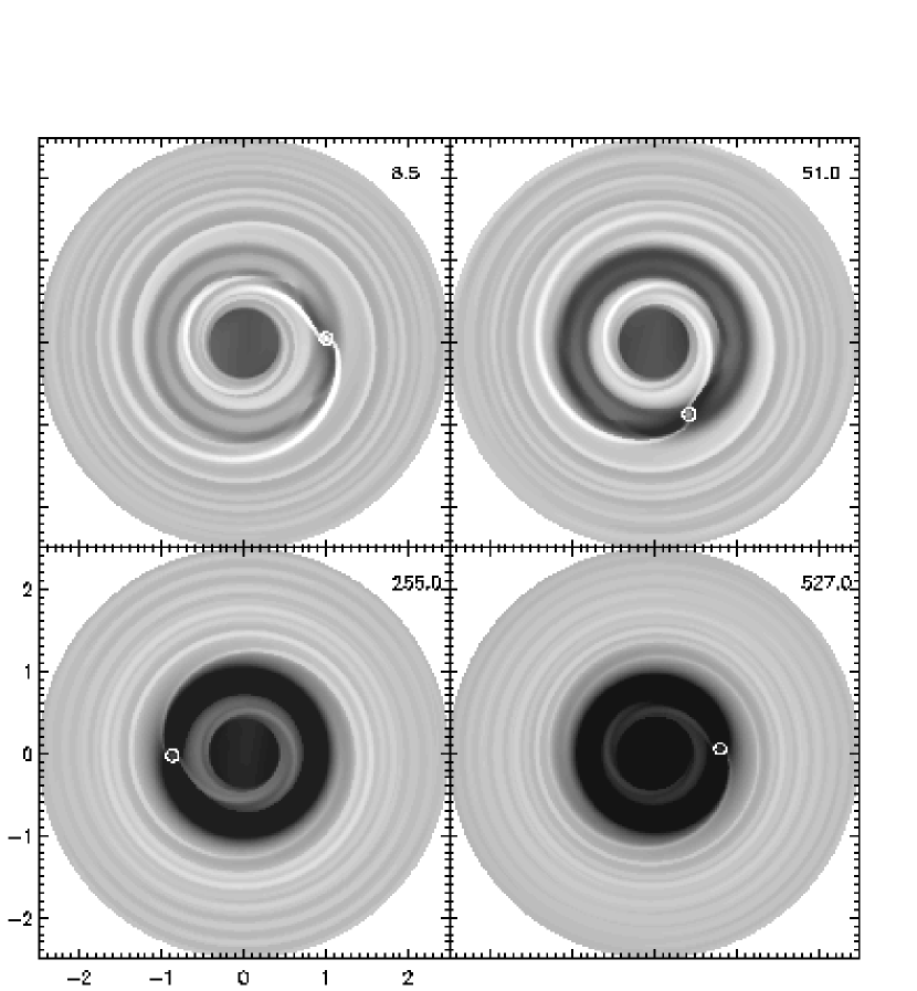
Figure 1: This figure shows the evolution of a protoplanet embedded in a protostellar disc for calculation N3. The relative surface density of disc material is represented by the grey-scale. The white circle represents the position of the protoplanet. The disc is initially unperturbed at time $t=0$.

5.1 NIRVANA

NIRVANA is a three dimensional MHD code that has been described in depth elsewhere (Ziegler & Yorke 1997). For the simulations presented here, the magnetic field is set to zero such that the code becomes purely hydrodynamic. We work in two dimensions and use cylindrical ($r$, $\phi$) coordinates. Viscous terms have been added as described by Kley (1998). The computational domain is subdivided into $N_{r}\times N_{\phi}$ zones, where the grid spacing in both coordinate directions is uniform.

For the calculations that are presented in this paper, three different levels of resolution have been used. The low resolution runs use $N_{r}=50$ and $N_{\phi}=147$, the mid–resolution runs use $N_{r}=80$ and $N_{\phi}=235$, and the high resolution runs use $N_{r}=130$ and $N_{\phi}=384$. The numerical method is based on a spatially second–order accurate, explicit method that computes the advection using the second order monotonic transport algorithm (Van Leer 1977), leading to the global conservation of mass and angular momentum. The evolution of the planet orbit is computed using a standard leapfrog integrator. NIRVANA has been applied to a number of different problems including that of an accreting protoplanet embedded in a protostellar disc. It was found to give results that are very similar to those obtained with other finite difference codes including RH2D (e.g. Kley 1999a).

5.2 FARGO

This is an alternative Eulerian ZEUS-like code, based on the FARGO fast advection method (Masset 1999). The main difference between NIRVANA and this code is that in FARGO the time step is not limited by the classical CFL condition, which results in a very small time step due to the fast orbital motion at the inner boundary, but it is limited by a CFL condition based on the residual velocity with respect to the average orbital motion. This leads to a substantially larger time step and hence faster computation. Also, the FARGO procedure leads to a smaller numerical diffusivity because a larger time step size requires one to perform fewer advection substeps during the calculations. Since the time step in the FARGO simulations can be quite large, especially in the low resolution case, a fourth-order Runge Kutta scheme was used to integrate the equations of motion of the protoplanet.

Since this work represents the first application of the FARGO advection algorithm, it has been widely tested against NIRVANA by running strictly similar simulations (identical physical and numerical parameters). The good agreement between both codes, along with the low numerical diffusivity of FARGO, have validated FARGO as a very useful tool for studying in the embedded protoplanet problem. Since it is much faster than NIRVANA, it has been used to calculate the very long-term behaviour of an accreting protoplanet (see run F6 below).

5.3 RH2D

To obtain results using a third method we have employed the code RH2D (Kley 1989). This has been used previously in studies of disc-protoplanet interaction (Kley 1998, 1999a). It is a two-dimensional radiation hydrodynamics code. For the simulations presented here the radiation module is switched off, and all parts are solved explicitly. The code is based on the second order Van Leer (1977) advection algorithm and uses a staggered grid, with logarithmic spacing (a constant enlargement ratio of neighbouring grid cells) in radius and which is uniform in azimuth. As in FARGO, a fourth order Runge Kutta scheme was used to integrate the protoplanet orbit. This code has already been found to give similar results to NIRVANA for protoplanet problems (Kley 1998). Accordingly we here use RH2D to study the orbital evolution of an embedded planet under slightly different conditions to those adopted in the case of the other two numerical methods.

6 Numerical Calculations

The main results of the numerical calculations are presented in table 1. Of particular significance are the migration times, $\tau_{mig}$, which are listed in the fifth column of table 1 in units of $10^{4}P_{0}$, and the estimated final masses of the planets, $m_{final}$, which are listed in the sixth column in units of the original planet mass $m_{init}.$

The values of $\tau_{mig}$ were obtained by measuring the rate of change of the planet’s semi-major axis at the end of the simulation and extrapolating forward in time assuming that this rate remains constant. Thus $\tau_{mig}$ gives as estimate of the time required for the planet to migrate all the way to the central star. The values of $m_{final}$ were obtained by measuring the accretion rate at the end of the simulation and extrapolating forward for a time $\tau_{mig}$.

Thus $m_{final}$ provides an estimate of the mass the planet will attain on migrating all the way to the central star. It should be noted that while these values provide reasonable estimates of the true migration times and accreted masses, the assumption of there being a constant migration or accretion rate is not strictly correct since these will tend to decrease as the planet mass continues to grow and migrate inwards. The only difference between runs N$i$ and F$i$ ($i\in[1,5]$) is the code used to perform the calculations, with the N$i$ runs being performed with NIRVANA and the F$i$ runs with FARGO. The evolution equations of the system and the initial conditions are identical. Their results agree reasonably well, except for the low resolution non accreting case, but as we shall see below, the low resolution we used for these runs is probably too coarse to give trustworthy results. From both the mid-resolution (N3 & F3) and high resolution (N5 & F5) runs, we can see that FARGO gives slightly higher accretion rates (and consistently longer migration times, since the inertia of the planet increases and, less importantly, most of the accreted material comes from the outer disk with a larger specific angular momentum). This higher accretion rate arises because FARGO has a smaller numerical diffusivity along the direction of orbital motion (Masset 1999). Associated with this is a more strongly peaked density profile around the planet.

Run	Resolution	Accretion	Initial	$\tau_{mig}$	$m_{final}$
	$N_{r}\times N_{\phi}$	on ?	Gap ?	$\times 10^{4}P_{0}$	($m_{init}$)
N1	$50\times 147$	Yes	No	1.77	4.8
N2	$50\times 147$	No	No	1.07	1.0
N3	$80\times 235$	Yes	No	1.00	3.2
N4	$80\times 235$	No	No	1.20	1.0
N5	$130\times 384$	Yes	No	0.84	2.7
N6	$130\times 384$	No	No	1.0	1.0
N7	$80\times 235$	Yes	Yes	0.45	3.25
N8	$80\times 235$	No	Yes	0.40	1.0
F1	$50\times 148$	Yes	No	1.99	4.77
F2	$50\times 148$	No	No	1.75	1.0
F3	$80\times 236$	Yes	No	1.08	3.85
F4	$80\times 236$	No	No	1.33	1.0
F5	$130\times 384$	Yes	No	0.85	3.27
F6	$70\times 180$	Yes	Yes	2.03	4.87
R1	$128\times 128$	(No)	Gap	1.45	1.0
R2	$128\times 128$	Yes	Gap	1.48	4.63
R3	$128\times 288$	Yes	Gap	1.36	4.10

Table 1: The first column gives the run label (N$i$ NIRVANA, F$i$ FARGO, R$i$ RH2D), the second column gives the number of grid cells used, and the third column indicates whether the planet accretes from the disc. The fourth column indicates whether the calculation started with an initial gap in the disc. The fifth column gives the estimated migration time (in units of $10^{4}P_{0}$) and the sixth column provides an estimate of the final mass of the planet. Note that the estimated times are given at different evolutionary times of the models.

For the purposes of illustrating the main results of our simulations, we will now describe the results for one individual case. Following this we will compare the results of simulations in which the disc either did or did not have a tidally induced gap in which the planet orbits at the start of the calculation. We will then go on to compare the migration rate of a planet which accretes gas from the disc at a maximal rate to that of a non accreting protoplanet. We then look at the effect of changing the initial surface density profile and disc aspect ratio. Following this, we compare the results obtained with NIRVANA and FARGO , and study the effects of changing the numerical resolution.

6.1 An Illustrative Case

Figure 2: This figure shows the torques (per unit mass) acting on the protoplanet during the early stages of its evolution, in run N3. The torque due to the disc exterior to the planet orbital radius $r_{p}$ is shown by the dotted line, that due to the disc interior to or at $r_{p}$ is shown by the dot-dashed line, and the torque due to the disc’s contribution to the indirect term of the gravitational potential is shown by the dashed line. The effective torque due to the accretion of disc gas is shown by the solid line.

The evolution of the protoplanet embedded in the disc for calculation N3 is shown in fig. 1, where grey-scale plots showing the surface density variation in the disc are presented, and the position of the planet is indicated by the small white circle (which has a radius equal to the Roche radius of the planet). Initially at time $t=0$ the disc surface density was unperturbed, but as the calculation proceeds the tidal force due to the planet strongly perturbs the disc, leading to the formation of trailing spiral shock waves. In particular an $m=2$ spiral wave pattern may be observed. The transfer of angular momentum between the disc and the protoplanet leads to the formation of an annular gap, or surface density depression, in the vicinity of the planet’s orbit, which is cleared after about 200 orbits for a Jupiter mass planet.

As the disc–planet system evolves, the inner disc is lost from the system since viscous evolution causes it to drain through the open inner boundary. The tidal interaction between the disc and protoplanet leads to the disc interior to $r_{p}$ exerting positive torques on the protoplanet, and the disc exterior to $r_{p}$ exerting negative torques on it. The loss of the inner disc leads to a reduction of the positive torque, so that the torque due to the outer disc becomes dominant. Consequently the planet undergoes inward orbital migration as its angular momentum is removed by the outer disc. In the final panel of fig. 1, which corresponds to a time of $t=527\;\;P_{0}$, it may be observed that the semi-major axis of the planet’s orbit is $\sim 80$ percent of it’s original value, and that most of the inner disc has disappeared. As the calculation proceeds beyond this point the planet continues to spiral in towards the central star.

The evolution of the torques acting on the protoplanet during the first 300 orbits are shown in fig. 2, and indicate what the dominant contribution to the orbital migration is. Here, the torque per unit mass acting on the protoplanet due to the disc exterior to the orbital radius of the protoplanet $r_{p}$ (dotted line), interior to, or at, $r_{p}$ (dot-dashed line), and the indirect term in the gravitational force (dashed line) are plotted against time. Also plotted is the effective torque per unit mass that arises from the accretion of material whose specific angular momentum differs from that of the orbit (solid line). The first thing to note is that the accretion of gas from the disc has a negligible effect on the orbital evolution. Once the gap has formed the effective torque arising from accretion is only $\sim 3$ percent of the torque due to the outer disc. Second, we note that the torque arising from the outer disc material is consistently larger than that due to the inner disc material. The loss of the inner disc through the open inner boundary causes this disparity in the torques to grow, and ensures that the migration is always directed inwards. The contribution that the disc gravity makes to the indirect term is found to have a negligible effect on the orbital evolution.

Figure 3: The first panel shows the evolution of the planet orbital radius for calculation N3 (solid line) and N7 (dotted line). The second panel shows the increase in mass as the protoplanets accrete gas from the disc for the same calculations, with the same line styles as described above.

The evolution of the orbital radius of the protoplanet is shown by the solid line in the first panel of fig. 3, and that of the planet mass is shown by the solid line in the second panel. The evolution of the protoplanet undergoes a more rapid phase early on as the planet loses angular momentum to the disc material during the gap opening phase, leading to a faster period of orbital migration. This phase of evolution lasts for a few hundred orbits until the gap is opened, and also results in a very large mass accretion rate that almost doubles the mass of the protoplanet within $t=300\;\;P_{0}$. Once the gap has been cleared, the evolution slows down and the planet spirals in towards the star at an almost constant rate while accreting gas from the disc at an almost steady accretion rate. The migration rate is observed to slow down slightly as the calculation proceeds since the increase in mass of the planet increases its inertia. The calculation was initiated with $M_{d0}\sim 2m_{p}$, but as the planet migrates and accretes from the disc we arrive at a situation where $m_{p}\geq M_{d0}$ (see discussion in section  2.2). The orbital evolution of a massive planet orbiting in a disc that contains a smaller mass than the planet within a characteristic radius $r_{p}$ has been studied by Ivanov, Papaloizou, & Polnarev (1999). In this physical regime the evolution is controlled by the viscous evolution of the disc and the inertia of the planet, with a more massive planet migrating more slowly, as described in section 2.2. We can test whether Eq. (9) agrees with our numerical calculations by examining the changes in planet mass, orbital radius, migration rate, and disc surface density at two different times, $t_{1}$ and $t_{2}$, during the calculation. If we allow for the reduction of the surface density in the outer disc due to accretion onto the planet, and by mass flow through the gap and through the inner boundary, then we obtain the following expression relating the migration rates ${\dot{r}}_{p}(t)$

$$\frac{{\dot{r}}_{p}(t_{1})}{{\dot{r}}_{p}(t_{2})}=\left(\frac{m_{p}(t_{2})\Sigma(t_{1})}{m_{p}(t_{1})\Sigma(t_{2})}\right)^{4/5}\left(\frac{r_{p}(t_{1})}{r_{p}(t_{2})}\right)^{3/5}$$ (22)

for a disc with a constant value of $\nu$. Comparing the migration rates in the numerical calculation at $t_{1}=1000\;P_{0}$ and $t_{2}=2000\;P_{0}$, we find reasonable agreement between the prediction of Eq. (22) and the numerical results. The measured ratio of the migration rates gives ${\dot{r}}_{p}(t_{1})/{\dot{r}}_{p}(t_{2})\simeq 1.5$, whereas that predicted by Eq. (22) gives a value ${\dot{r}}_{p}(t_{1})/{\dot{r}}_{p}(t_{2})\simeq 1.4$ with $\Sigma$ taken as the azimuthally averaged value at the location of the 2:1 outer Lindblad resonance.

The accretion rate decreases as the protoplanet mass increases because the disc is tidally truncated more effectively by a more massive planet (e.g. BCLNP) After a time of $t\sim 2400\;\;P_{0}$, the protoplanet has migrated to a radius of $r\sim 0.6$ and has accreted $\sim 1.3$ times its original mass. By extrapolating the migration and accretion rates forward in time, it is estimated that the planet will spiral into the central star after $t\sim 1.0\times 10^{4}\;\;P_{0}$, by which time it will have reached a mass $m_{final}\sim 3.2$ times its original mass.

We note that the planet remains in an almost circular orbit throughout its evolution, and shows no sign of eccentricity growth, since the gap region still contains sufficient corotating material that is able to damp the eccentricity growth caused by the outer Lindblad resonances (Goldreich & Tremaine 1980, Artymowicz 1993a,b).

The viscous evolution time of the disc is given by Eq. (6). At a radius of $r=1$, this corresponds to an evolution time of $\sim 10^{4}\;\;P_{0}$, very similar to what is observed for the migration time of the protoplanets in all of our simulations.

This confirms the idea described in section 2.2 and in Lin & Papaloizou (1986) that giant protoplanets undergoing tidal interaction with a protostellar disc should migrate on a time controlled by the viscous evolution time of the disc when the interaction is sufficiently non linear to open up a gap, and when the mass of the planet is less than or comparable to the disc mass with which it gravitationally interacts.

6.2 The Effects of an Initial Gap

As well as performing calculations in which the initial disc was unperturbed, we also performed calculations in which the initial disc contained a tidally induced gap around the vicinity of the planet. Here we will concentrate on the calculations labelled as N3 and N7 in table  1.

The calculation labelled as N3 is for an accreting protoplanet embedded in an initially unperturbed disc, and was described in detail in the previous section 6.1. The calculation labelled as N7 in table 1 is for an accreting protoplanet initially embedded in a disc which has a tidally induced gap at time $t=0$. This initial condition was obtained by running a calculation with a non accreting planet on a fixed circular orbit for $t\sim 300\;P_{0}$, until a clear gap was formed and the surface density in the gap region became steady. A reflecting inner boundary condition was employed during this phase in order that the disc mass was conserved. The results of this calculation were then used as the initial conditions of calculation N7, but now with an accreting protoplanet which was able to undergo orbital evolution, and with an open inner boundary condition.

The evolution of the orbital radius of the planet in calculation N7 is shown by the dotted line in the first panel of fig. 3, and the evolution of the mass of the planet is shown by the dotted line in the second panel. In the case of the calculation N3, in which the planet is initially embedded in an unperturbed disc and must clear material in order to form a gap, the clearing of that material leads to a period of more rapid migration. At the same time, this larger migration rate is slowed by the rapid accretion of gas, when the planet is deeply embedded, that leads almost to a doubling of the planet mass and inertia within a few hundred orbits. In the case of calculation N7, the planet initially resides within a gap, and so does not have to clear much material away from its vicinity during the early stages of its orbital evolution. It does, however, have an early period of more rapid accretion since it absorbs the material that is initially within its Roche lobe that accumulated there during the formation of the gap. This initially large accretion rate is augmented by the fact that an accreting planet helps to reduce the surface density of material in the gap region by accreting some of it. The similarity of the migration rates for the calculations N3 and N7 during the first $1000\;P_{0}$ indicates that the effects of opening the gap for an initially fully embedded planet are almost entirely counter balanced by the planet mass growth and accretion of material with a higher specific angular momentum, with this latter effect being almost negligible after $\sim 100\;P_{0}$ (as shown in fig. 2).

Looking at the the later stages of the evolution in the first panel of fig. 3, we notice that although the planet in calculation N3 migrates slightly faster to begin with, the planet in calculation N7 eventually migrates at a higher rate since its mass and inertia are smaller, with the orbital radii crossing over at $t\sim 1500\;P_{0}$. The expected migration time scale in calculation N7 is $\tau_{mig}\sim 0.45\times 10^{4}\;P_{0}$, with the final mass estimate being $m_{final}\sim 3.2$, indicating that the presence or not of an initial gap has only a relatively small effect on the final results.

6.3 Comparison of the Evolution of an Accreting and Non Accreting Protoplanet

Calculations were performed for both accreting and non accreting planets. In this section we will compare the results of calculations N3 and N4 in order to ascertain the effects of accretion on the evolution of the protoplanet. These calculations were both initiated with unperturbed disc models. For the accreting protoplanets, the accretion rate adopted is such that the e–folding time for the protoplanet to accrete mass within a distance of half of its Roche radius is given by $\tau_{acc}=3P_{0}/(2\pi).$ This is a dynamical time scale so the situation corresponds essentially to a maximally accreting protoplanet (Kley 1999a).

The case of a non accreting planet corresponds to the situation where the protoplanet has a lobe filling gaseous envelope in hydrostatic equilibrium with Kelvin–Helmholtz time longer than the migration time. Then the planet can accrete little mass during the migration stage. Such a situation may occur if the envelope is built up while maintaining a low luminosity emitted from the central parts of the protoplanet.

Figure 4: This figure shows the evolution of the orbital radius for the accreting protoplanet in run N3 (solid line) and for the non accreting protoplanet in run N4 (dotted line).

Calculation N3 was discussed in some detail in section 6.1. Fig. 4 shows the evolution of the orbital separations for calculations N3 (solid line) and N4 (dotted line). It is apparent that the non accreting planet (N4) undergoes a significantly more rapid phase of migration as the initial gap is cleared during the first few hundred orbits, since the planet has to transfer a substantial amount of angular momentum to the disc gas in order to clear the gap. The rapid accretion of mass (and some angular momentum) by the accreting planet (N3) helps to counteract the initial inward torques that arise when the gap is being cleared of material, as described in section 6.2.

As the calculations proceed, the migration rates in both cases slow down when the gap has been cleared of material. The planet then migrates inwards on approximately the viscous evolution time scale of the outer disc. Some additional slowing down of the migration rates occurs because the protoplanets interact with a smaller amount of disc mass as they migrate inwards.

As the evolution time approaches $t=2000\;P_{0}$, it is apparent that the migration rate of the non accreting planet is actually slower than that of the accreting planet, even though the accretion of material has increased the inertia of the accreting planet. The reason for this unexpected behaviour is that the non accreting planet undergoes Roche lobe overflow. As material accumulates onto the non accreting planet, the Roche lobe eventually becomes filled with a hydrostatic atmosphere and no additional material may enter it. The continued flow of material from the outer disc onto the protoplanet then leads to circulation around it and Roche lobe overflow, such that material flows towards the central star.

This material contains too much angular momentum to flow through the inner boundary directly, and instead fuels the inner disc. This inner disc then exerts a positive torque on the planet and reduces the rate at which it is able to migrate towards the central star. This process provides an efficient method of allowing material to flow across tidally induced gaps in accretion discs, and thus for the outer disc to feed material in to the inner disc which can continue to accrete onto the central star. This process will be the subject of a more detailed future study.

Figure 5: This diagram shows the distance between the protoplanet and the primary as a function of time in run F6. At $t=0$ the gap is already cleared (it was cleared during 400 fixed circular orbits).

6.4 A Long-term Evolution Run

The run F6 is a low/mid-resolution run aimed at computing the long-term behaviour of the accretion/migration process. As indicated in table 1, $N_{r}=70$ and $N_{\phi}=180$. Contrary to the other FARGO and NIRVANA runs, the inner boundary is located at $r=0.25$ instead of $r=0.4$, and the radial grid spacing is in geometric progression rather than uniform. Since we want to deal with the long-term behaviour of the protoplanet, we allow it to get close to the primary which is why we take a smaller inner boundary radius. Furthermore, we want to track the accretion rate as accurately as possible. Taking the non uniform radial grid spacing ensures that the cells all have the same shape and that the accretion algorithm will not be biased accordingly. For this run we first clear the gap with the inner boundary open by evolving the system with the protoplanet orbit circular and fixed for 400 periods. Then we start the accretion/migration process. Time $t=0$ is taken then.

In this run, as distinct from the others, the frame is centered on the centre of mass of the system composed of the primary and the protoplanet. This is not an inertial frame, since that would need to be centered on the centre of mass of the primary, protoplanet and disc. But the indirect term arising from the acceleration of this frame is much smaller than the indirect term in the case of a frame centered on the primary. Furthermore, the material in the outer disk tends to orbit around the centre of mass of the primary and protoplanet (since the disk itself is not self-gravitating), so one can work with a rigid outer boundary and impose there a fixed Keplerian velocity, with no radial motion, which avoids inflow and outflow at that boundary. On the other hand, the material in the inner disk tends to orbit around the primary, so there is a mismatch there between the grid boundary and the gas orbits, which leads to a “vacuum-cleaner” effect which drains the inner disk faster than a frame centered on the primary would do. However, tests have shown that the flux of mass at the inner boundary is at most 10 to 20 % larger as a result of this effect.

We present in figure 5 the evolution of the protoplanet-primary separation as a function of time. In figure 6 we show the total mass of the protoplanet as a function of time, and in table 1 we give the estimated migration time and final masses. These rates have been extrapolated from the time derivatives of the mass and orbital radius at time $t=7500$. This corresponds roughly to the time at which the inner disk is lost. The fact that these results are in relatively good agreement with the previous ones, even though the extrapolation is performed after many more orbits in the case of run F6, shows that assuming that the migration and accretion rates reach constant values is a reasonable approximation, even though the curves show some residual deviation from linearity.

Figure 6: This figure shows the temporal behaviour of the protoplanet mass as a function of time in run F6. We notice that the curve slope (i.e. the accretion rate) is not very peaked at $t=0$ since the gap was already present. The mass unit is one Jupiter mass.

We show in figure 7 a sequence of four surface density plots at times ($t=0$, $t=300$, $t=3000$, $t=7000$). As a consequence of the migration the gap radius decreases with time. We note as well the depletion of the inner disc (the viscous time scale at $r=0.7$ is $\tau_{\rm visc}=7.8\cdot 10^{3}$ orbits, and is even smaller at smaller radii).

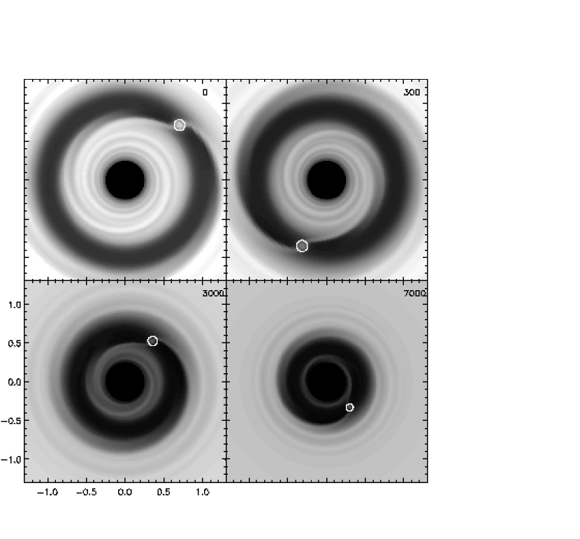
Figure 7: Time sequence of the surface density for run F6. The outer boundary is at $2.5$ and does not appear on the plots. The circle around the protoplanet in each case has a radius equal to the Roche radius.

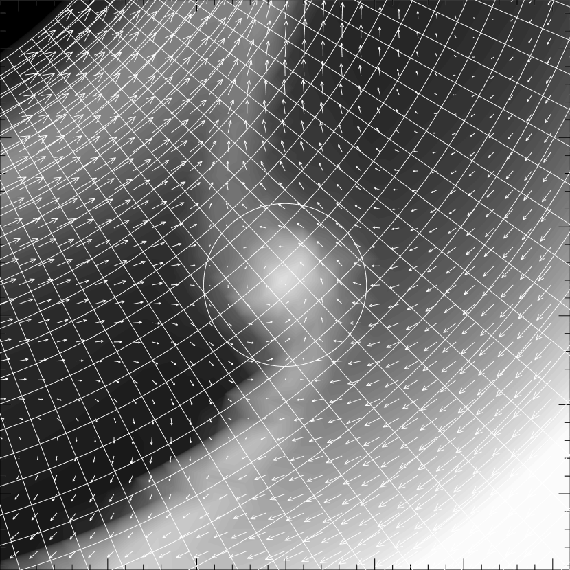
Figure 8: Details of the flow in the neighbourhood of the protoplanet near the end of the run F6 ($t=7000P_{0}$). The velocity field is represented in the frame corotating with the planet. We clearly see the gap, the wakes of the protoplanet in the inner and outer disk, the extremities of the horseshoe orbits in the gap, the two X-points in the velocity field, which correspond to the Lagrange points L₁ and L₂. The circle is centered on the protoplanet and has a radius equal to the Roche radius of the protoplanet. Because the actual potential felt by the disk material is smoothed, the X-points lie slightly inside this circle. One can see that the density peak around the planet is not elongated along the orbit, as usually observed in fixed frame normal advection scheme runs. Because of the geometric grid spacing, all the cells have the same shape and are “as square as possible”, i.e. $\log(r_{out}/r_{in})\simeq N_{r}\log(1+2\pi/N_{\phi})$.

Fig. 8 shows the flow around the protoplanet at the end of the run. Even though the inner disk is strongly depleted, some Roche lobe overflow into it is indicated. The mean profile of the gap surface density at different times is displayed in fig. 9. The gap deepens as the protoplanet mass increases with time. The depletion of the inner disc is also apparent.

Figure 9: Disk surface density profile at different times for run F6 ($t=0$ : solid line, $t=690$ : dotted line, $t=1830$ : dashed line and $t=3550$ : dot-dashed line). These plots represent the azimuthal average of the surface density, and hence take the protoplanet wake into account. The residual surface density which would be obtained by omitting the wakes would be much smaller.

The mass lost through the inner boundary as a function of time is plotted in fig 10. From the comparison of figs. 6 and 10, one can see that the mass overflow flux and the mass accretion rate onto the planet have the same order of magnitude (the mass overflow flux is of the same order of magnitude as the mass outflow through the inner boundary since the mass lost at the inner boundary is bigger than the inner disk mass; in a totally stationary case these two rates would be strictly equal).

Figure 10: Mass lost at the inner boundary as a function of time in run F6. At $t=0$ this mass is not zero since the run was begun with a non-accreting protoplanet on a fixed circular orbit with an open inner boundary in order to generate an initial gap.

The value of the ratio of the mass flow rate through the gap to the accretion rate $\sim 1/3.5$ obtained here is somewhat higher than that obtained from the simulation $R2$ where this ratio was about $1/7.$ However, the magnitude of the accretion rate is smaller here since the planet mass is larger. Also the surface density profiles and disk aspect ratios are different in these simulations. Given the differing physical situation when the accretion rates were measured, we consider the agreement to be satisfactory.

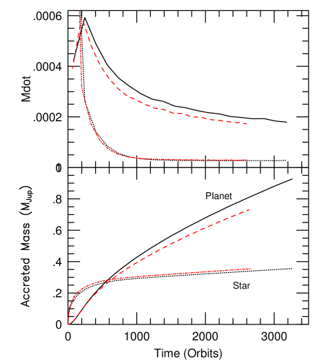
Figure 11: Mass evolution for models $R2$ and $R3$: The lower panel shows the evolution of the mass of the planet and the mass lost from the disc (accreted by the star). The top panel shows the corresponding accretion rates in units of $M_{J}/P_{0}$. Dark solid and dotted lines refer to model R2, while the lighter dashed and dashed-dotted lines refer to the higher resolution model R3.

6.5 Runs with an Initial Surface Density Profile Using RH2D

The code RH2D has been already been tested against NIRVANA (Kley 1998) and found to give very similar results so we shall not give results of additional tests here. Instead we present runs R$i$ ($i=1,2,3$) which use different initial conditions incorporating a surface density profile that is not constant, as outlined at the end of section 4.6, and a slightly higher value of the disc aspect ratio $H/r=0.05$. Also, it should be noted that these calculations are initiated with a gap already in existence around the position of the protoplanet.

The main results concerning the mass accretion by the protoplanet are displayed in Fig. 11. The lower panel shows the evolution of the protoplanet mass and the mass lost through the inner boundary for the models R2 and R3 which have maximal accretion. These models have the same physical setup but different numerical resolutions. Note that only the mass added to the planet during the evolution is displayed. The total planet mass is obtained by adding $1M_{J}$ to the quoted values, i.e. at the end of the run R2 at $t\approx 3300$ the planet has reached about $2M_{J}$. This value is smaller than that obtained by the other codes (see for example run F6), which is a result of the surface density near the planet being a factor of about three smaller in these runs. Also shown in the lower panel is the mass lost through the inner boundary (dotted and dashed dotted lines) which is assumed to have been accreted by the star. The mass of the planet rises more slowly initially, because of the initial gap imposed. Only after the full development of the quasi-stationary flow (at $t\approx 300$) does the mass accumulation rate onto the planet become larger than the mass loss rate through the inner boundary. This is demonstrated in the top panel where the mass accretion rates in units of $M_{J}/P_{0}$ onto the planet and star are shown. After the mass contained initially within $r=0.25$ and $0.4$, $M_{d0}=0.37M_{J}$ is consumed (primarily by the star), the mass accretion rate onto the star settles to the very small constant value $\dot{M}_{lost}=2.86\times 10^{-5}M_{J}/P_{0}$ which may be identified with the rate of mass overflow across the gap. Near the end of the computation at $t=3000$ this rate is about 6.5 times lower than the mass accretion rate by the planet which is in rather good agreement with the results quoted in Kley (1999a) but somewhat lower than the rates obtained with FARGO as outlined above.

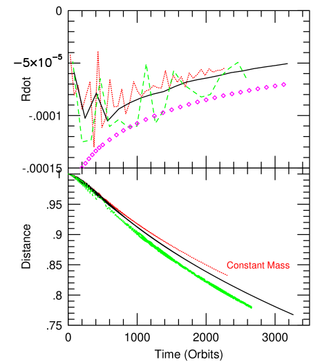
Figure 12: Radial evolution for models R$i$: The lower panel shows the evolution of the semi major axes of the planet for three different models. Solid black line R2, dotted grey line the non-accreting model R1, and dashed light grey line the high resolution model R3. The top panel shows the corresponding derivative $\dot{r}_{p}$ in units of $a_{0}/P_{0}$ versus time. The diamonds represent the analytical approximation according to Ivanov, Papaloizou, & Polnarev (1999) as given in Eq. 9 for model R2.

In Fig. 12 the evolution of the distance of the planet from the star is shown for all models R1–R3. Again, due to the smaller mass contained in the physical domain the orbital decay rate is smaller than in the previous models (N$i$ and F$i$). In the comparison model labeled ‘constant mass’ (R1, dotted line) the mass of the planet remained constant but mass was nevertheless removed from the Roche–lobe in the manner described in section 4.5 (also see Kley, 1999a). This model has a smaller decay rate than the complete models (R2 solid line, and R3, light dashed line) in which the accreted mass is added to the planet mass. All the models show initially a fluctuation in $r_{p}(t)$ which indicates an eccentricity growth to less than about 0.02 which damps out at later times. For the high resolution model (R3, light dashed line) the radial evolution follows closely the low resolution model, the migration rate seems to be marginally lower. This is consistent with the results obtained with NIRVANA and FARGO which indicate that lower resolution runs have larger accretion rates and slower decay rates (see Figs. 15 and 16).

The diamonds in Fig. 12 represent the analytical approximation according to Ivanov, Papaloizou, & Polnarev (1999) as given in Eq. 9 with an arbitrary normalisation factor which can be adjusted to match the numerically obtained data. For simplicity here the maximum of the azimuthally averaged surface density $\Sigma(r)$ outside of the planet was taken for model R2 as the value for the surface density in (9). Clearly the formula gives an excellent approximation to the actual evolution of the radius of the planet.

6.6 Comparison between NIRVANA and FARGO

Figure 13: The first panel shows the evolution of the planet orbital radius, with calculation N3 being represented by the solid line and F3 by the dotted line. The second panel shows the increase in mass as the planet accretes gas from the disc, with the same line styles representing the two calculations.

In this section we present the results of calculations that were performed with both NIRVANA and FARGO in order to check that the results that we have presented are reproducible when using independent numerical codes. The calculations that we will compare are N3 performed using NIRVANA and F3 performed using FARGO. As described in table 1, these calculations are for an accreting Jupiter mass planet initially embedded in an unperturbed disc model. For comparison purposes, the orbital evolution of the protoplanet is plotted in the first panel of fig. 13, with calculation N3 being represented by the solid line and F3 being represented by the dotted line. Similarly, the evolution of the protoplanet mass is presented in the second panel of this figure with the same line styles being used to represent the calculations. It is apparent that the results are very closely matched in terms of the orbital evolution rate and reasonably well matched in terms of the mass accretion rates. We clearly see the trend, also seen in the results given in table 1, that the FARGO algorithm gives higher accretion rates and hence slightly slower migration. This may be related to the fact that the distribution of matter close to the protoplanet is subject to less numerical diffusion and so has less azimuthal elongation in FARGO.

6.7 Numerical Resolution

6.7.1 Non accreting planets

In this section we present the results of calculations that were performed using different resolutions. We first concentrate on comparing three calculations in which the orbital evolution of a non accreting planet was studied, namely calculations N2, N4, and N6.

Figure 14: This figure shows the evolution of the orbital radius for the calculations N2 (dotted line), N4 (solid line), and N6 (dashed line). The resolution for each calculation is described in table 1.

The evolution of the planet orbit radius for these calculations is presented in fig. 14, with calculation N2 being represented by the dotted line, calculation N4 by the solid line, and calculation N6 by the dashed line. The agreement between N2 and the other calculations appears to be the worst, which is to be expected since this is the lowest resolution simulation that we performed and this is probably too low to fully resolve small scale structures in the vicinity of the planet. The two calculations N4 and N6 on the other hand show extremely good agreement in their orbital migration rates at later times, though there is a small offset in the orbital radius at any given time due to calculation N6 experiencing more rapid migration during the gap clearing stage of the calculation.

This increased rate of orbital migration for the higher resolution calculation during the gap clearing stage probably arises because of its ability to resolve density waves with higher azimuthal mode numbers that are located close to the planet when it is embedded. Once the gap has been cleared, however, these non axisymmetric structures do not provide a significant contribution to the tidal torque acting on the planet, so that the migration rates then become approximately equal. The close agreement between the migration rates of calculations N4 and N6 indicate that our calculations have essentially reached convergence in their results.

6.7.2 Accreting planets

Figure 15: The first panel shows the evolution of the orbital radius for the calculations N1 (dotted line), N3 (solid line), and N5 (dashed line). The evolution of the planet mass is shown in the second panel, with the line styles being the same as above. The resolution for each calculation is described in table 1.

Figure 16: Same as figure 15 for FARGO results F1 (dotted line), F3 (solid line) and F5 (dashed line).

The calculations for accreting planets initially embedded in unperturbed accretion discs that were performed with different resolutions are shown in figs. 15 and 16. The first panel in fig. 15 shows the orbital radius as a function of time for the calculations N1 (dotted line), N3 (solid line), and N5 (dashed line). The second panel shows the evolution of the planet mass, with the same line styles as described for the first panel.

Fig. 16 gives the corresponding results for the runs F1, F3 and F5. It is apparent that the lower resolution runs have a larger accretion rate. This leads to smaller migration rates because the protoplanets have larger masses. Nonetheless, the migration times obtained for these runs all indicate an orbital decay time of $\tau_{mig}\sim 10^{4}\;P_{0}$, as indicated in table 1. This is in agreement with the idea that the orbits of giant planets will evolve on the viscous diffusion time of the protostellar disc. The results of NIRVANA and FARGO are in good agreement with respect to migration rates and final planetary masses. The predicted final planetary masses in the calculations N3 and N5 are $3.2M_{J}$ and $2.7M_{J}$ while for the calculations F3 and F5 they are $3.85M_{J}$ and $3.25M_{J}$ respectively. These agree well with the estimated masses of a number of the recently discovered closely orbiting extrasolar giant planets (Marcy, Cochran, & Mayor 1999, Marcy & Butler 1998).

7 Discussion and Conclusion

In this paper we have studied the interaction of a protoplanet of $1M_{J}$ initially with a gaseous disc whose aspect ratio and kinematic viscosity are those expected for a minimum mass solar nebula. This had characteristically $2M_{J}$ interior to the initial circular orbit radius of the protoplanet. The problem was studied with three independent hydrodynamic codes, NIRVANA, FARGO and RH2D. These were found to give consistent results when compared. FARGO had the additional advantage that, on account of the fast advection scheme employed, the evolution could be followed for a much longer time.

A general result of the simulations was that the direction of the orbital migration was always inwards and such that the protoplanet reached the central star in a near circular orbit after a time of $\sim 10^{4}$ initial orbital periods, which is characteristically the viscous time scale at the initial orbital radius. This was found to be independent of whether the protoplanet was allowed to accrete mass or not, or the surface density profile in the disc. The tendency to migrate inwards was assisted by the disappearance of the inner disc through accretion onto the central star. When the protoplanet was allowed to accrete at a near maximal rate the mass was found to increase to about $4M_{J}$ as it reached the central star. Because of deep gap formation and lower accretion rates for the larger masses (also see BCLNP) it is difficult to exceed this mass in the kind of simulations presented here. An additional calculation has been performed with an initial planet mass of $3M_{J}$, but whose results are not described here in detail. This calculation resulted in a similar migration time of $\sim 10^{4}\;P_{0}$, and an estimated final mass for the protoplanet of $4.8\;M_{J}$, indicating the difficulty of forming giant planets with masses greater than about 5 $M_{J}$ before they have migrated to the centre. It would appear that the masses estimated for a number of close orbiting giant planets (Marcy, Cochran, & Mayor 1999, Marcy & Butler 1998) as well as their inward orbital migration can be explained by the operation of the processes considered here during the late stages of giant planet formation.

Several important issues, however, remain to be resolved. The inward migration time is shorter than previously estimated time scales $\sim 10^{6}$ yr for the formation of a Jovian mass protoplanet (e.g. Bodenheimer & Pollack 1986; Pollack et al. 1996; Papaloizou & Terquem 1999). This is suggestive that either the planet formation process may be speeded up by the earlier merger of cores undergoing type I migration, and/or there may be regions in the disc where the viscosity is very small, so halting type II migration, perhaps due to inadequate ionization for MHD instabilities to operate. Additional planets embedded in the disc alter the density structure and consequently the torque balance which may result in a halting of the migration process (Kley 1999b). Many body processes such as gravitational scattering of protoplanets may also operate to move them to different orbital locations in the disc (e.g. Weidenschilling & Marzari 1996).

An additional possibility is that in some cases giant planet formation occurs at substantially larger distances from the host star than have hitherto been given serious consideration. For example, a planet forming at a radius $\sim 20$ AU will have a migration time of $\raisebox{-3.44444pt}{$\buildrel\textstyle>\over{\sim}$}\;10^{6}$ yr, which is now within the estimated range of lifetimes of protostellar discs around T Tauri stars (i.e. $10^{6}$ – $10^{7}$ yr). It is possible that inward migration of these protoplanets may simply be halted by the eventual dissipation of the disc at the end of the T Tauri stage. The final orbital positions of these planets will then be determined by the initial radius at which the planets were formed and the age at which the T Tauri phase ends. In this scenario, planets that initially start to form closer in towards the central star (e.g. at 5 AU) will migrate inwards and will become ‘hot Jupiters’, whereas those planets that form further away stand a much greater chance of being at intermediate distances from their host stars when orbital migration is halted by the disappearance of the disc.

Another issue is that type II migration in a viscous disc as considered here tends to cause Jovian mass protoplanets to merge with their central star on a time scale short compared to the lifetime of protostellar discs. Thus a process for halting the migration is required. This may occur through the termination of the inner disc due to a magnetospheric cavity (Lin, Bodenheimer, & Richardson 1996).

The calculations presented here make a number of important assumptions that may have some bearing on the final results obtained. By using a locally isothermal equation of state, we tacitly assume that any heat generated by the spiral shock waves is immediately radiated from the system. This may not be an accurate description of the thermodynamics, and if radiative processes operate on a time scale that is longer than the orbital time scale then some thickening of the disc may result. In addition, we assume that the turbulent viscosity can be simply modeled using the Navier-Stokes equation, when in reality it should arise naturally from MHD instabilities. These, and other assumptions can only be addressed by performing global simulations that include radiative and MHD processes in three dimensions. We hope in the near future to be able to address some of these outstanding issues.

8 Acknowledgements

This work was supported in part (F.M.) by the European Commission under contract number ERBFMRX-CT98-0195 (TMR network “Accretion onto black holes, compact stars and protostars”), and by the Max-Planck-Gesellschaft, Grant No. 02160-361-TG74 (for W.K.). Computational resources of the Max-Planck-Institute for Astronomy in Heidelberg were available and are gratefully acknowledged. We thank Udo Ziegler for making a FORTRAN Version of his code NIRVANA publicly available.

References

- [1993a] Artymowicz, P., 1993a, ApJ, 419, 155
- [1993b] Artymowicz, P., 1993b, ApJ, 419, 166
- [1991] Balbus, S.A., Hawley, J.F., 1991, ApJ, 376, 214
- [1998] Balbus, S.A., Hawley, J.F., 1998, Rev. Mod. Phys. 70, 1
- [1996] Beckwith, S.V.W., Sargent, A., 1996, Nat, 383, 139
- [1997] Bell, K.R., Cassen, P.M., Klahr, H.H., Henning, Th, 1997, ApJ, 486, 372
- [1986] Bodenheimer, P., Pollack, J.B., 1986, Icarus, 67, 391
- [1999] Bryden, G., Chen, X., Lin, D.N.C., Nelson, R.P., Papaloizou, J.C.B, 1999, ApJ, 514, 344
- [1996] Gammie, C.F., 1996, ApJ, 462, 725
- [1978] Goldreich, P., Tremaine, S., 1978, ApJ, 222, 850
- [1979] Goldreich, P., Tremaine, S., 1979, ApJ, 233, 857
- [1980] Goldreich, P., Tremaine, S., 1980, ApJ, 241, 425
- [1999] Ivanov, P.B., Papaloizou, J.C.B., Polnarev, A.G., 1999, MNRAS, 307, 79
- [1989] Kley, W., 1989, A&A, 208, 98
- [1998] Kley, W., 1998, A&A, 338, L37
- [1999a] Kley, W., 1999a, MNRAS, 303, 696
- [1999b] Kley, W., 1999b, MNRAS, , submitted
- [1996] Korycansky, D.G., Papaloizou, J.C.B., 1996, ApJ, 105, 181
- [1996] Lin, D.N.C., Bodenheimer, P., Richardson, D.C., 1996, Nat, 380, 606
- [1979a] Lin, D.N.C., Papaloizou, J.C.B., 1979a, MNRAS, 186, 799
- [1979b] Lin, D.N.C., Papaloizou, J.C.B., 1979b, MNRAS, 188, 191
- [1980] Lin, D.N.C., Papaloizou, J.C.B., 1980, MNRAS, 191, 37
- [1985] Lin, D.N.C., Papaloizou, J.C.B., 1985, Protostars and Planets II, 981, Tucson, AZ, University of Arizona Press.
- [1986] Lin, D.N.C., Papaloizou, J.C.B., 1986, ApJ, 309, 846
- [1993] Lin, D.N.C., Papaloizou, J.C.B., 1993, Protostars and Planets III, 749
- [1993] Lissauer, J.J., Stewart, G.R., 1993, Protostars and Planets III, 1061
- [1998] Marcy, G.W., Butler, R.P., 1998, ARA&A, 36
- [1999] Marcy, G.W., Cochran, W.D., Mayor, M., 1999, To appear in Protostars and Planets IV.
- [1999] Masset, F.S., 1999, A&A, , Submitted.
- [1984] Papaloizou, J.C.B., Lin, D.N.C., 1984, ApJ, 285, 818
- [1999] Papaloizou, J.C.B., Terquem, C., 1999, ApJ, 521, 823
- [1999] Papaloizou, J.C.B., Terquem, C., Nelson, R.P., 1999, Astrophysical Discs – An EC Summer School, 186, Astronomical Society of the Pacific, Conference Series Vol. 160, Eds. J.A. Sellwood, J. Goodman
- [1996] Pollack, J.B., Hubickyj, O., Bodenheimer, P., Lissauer, J.J., Podolak, M., Greenzweig, Y., 1996, Icarus, 124, 62
- [1973] Shakura N.I., Sunyaev R.A., 1973, A&A, 24, 337
- [1995] Syer, D., Clarke, C.J., 1995, MNRAS, 277, 758
- [1977] Van Leer, B., 1977, J. Comp. Phys., 23, 276
- [1997] Ward, W.R., 1997, Icarus, 126, 261
- [1996] Weidenschilling S.J. & Mazari F., 1996, Nat, , 384, 619
- [1997] Ziegler U., Yorke H.W., 1997, Comp. Phys. Comp., 101, 54