Pulsar Magnetospheric Emission Mapping:
Images and Implications of Polar-Cap Weather

Abstract

The beautiful sequences of “drifting” subpulses observed in some radio pulsars have been regarded as among the most salient and potentially instructive characteristics of their emission, not least because they have appeared to represent a system of subbeams in motion within the emission zone of the star. Numerous studies of these “drift” sequences have been published, and a model of their generation and motion articulated long ago by Ruderman & Sutherland (1975); but efforts thus far have failed to establish an illuminating connection between the drift phemomenon and the actual sites of radio emission. Through a detailed analysis of a nearly coherent sequence of “drifting” pulses from pulsar B0943+10, we have in fact identified a system of subbeams circulating around the magnetic axis of the star. A mapping technique, involving a “cartographic” transform and its inverse, permits us to study the character of the polar-cap emission “map” and then to confirm that it, in turn, represents the observed pulse sequence. On this basis, we have been able to trace the physical origin of the “drifting-subpulse” emission to a stably rotating and remarkably organized configuration of emission columns, in turn traceable possibly to the magnetic polar-cap “gap” region envisioned by some theories.

Since their discovery by Drake & Craft (1968), “drifting” subpulses have fascinated both observers and theorists and have often been regarded as one of the “keys” to understanding pulsar radio emission. Without any adequate model, early studies of prominent “drifters” (e.g., Taylor & Huguenin (1971); Backer (1973)) focussed on delineating the drift phenomenon. Then, Ruderman & Sutherland’s (1975) model not only articulated a qualitative picture of “drifting” subpulses as a system of “carousel beams” circulating around the magnetic axis within the (magnetic) polar emission region, but they also attributed the rotation physically to E$\times$B drift and estimated how long these circulation times would be.

While fascinating and theoretically compelling, the phenomenon has proved difficult to interpret physically. No such sequence has appeared precise enough to determine the structure and dynamics of the beams, and thus to see if it follows any pattern which might or might not confirm the expectations of the aformentioned model. Any sightline to a star can cross the periphery of its polar emission cone at only one or two points, and it was difficult to fix accurately just where these points fell in relation to the rotational and magnetic axes. Nor was it clear to what extent the “drift” rates were aliased by the rotation frequency of the star. Within the Ruderman & Sutherland model, the total number of subbeams must be ascertained, or no calculation of the circulation time is possible—and thus no quantitative connection can be made with theories of the polar-cap “gap” region. It is a telling statement on this unfortunate state of affairs that the most extensive studies of a pulsar with a highly regular “drifting”-subpulse pattern, B0809+74, were published 25-30 years ago! [Taylor et al. (1971); Manchester et al. (1975)].

Pulsar B0943+10 is another pulsar in the same class and is remarkable in other ways as well. One of a handful of pulsars discovered below 300 MHz (Vitkevich, et al., 1969), it weakens markedly at higher frequencies and has never been detected above 600 MHz. Its profile evolution (and “drifting” subpulses) identify it as a member of the conal single ($S_{d}$) class (Rankin, 1993b), and we now know that its steep spectrum is due to a sightline traverse so peripheral that it ultimately misses the ever narrower high frequency cone. The pulsar’s long sequences of “drifting” subpulses have prompted several different studies [Taylor & Huguenin (1971); Backer et al. (1975); Sieber & Oster (1975)]—all showing strong fluctuations at a frequency of 0.46 cycles per rotation period (hereafter, c/$P_{1}$) and a weaker feature near 0.07 c/$P_{1}$. Two profile “modes” also have been identified, a “B” (for “bright”) mode in which subpulse “drift” is very prominent, and a “Q” (for “quiescent”) mode wherein the subpulses are weaker and disorganized [Suleymanova & Izvekova (1984); Suleymanova et al. (1998)]. For all these reasons the pulsar’s subpulse sequences are difficult to observe, and our study is based on 430-MHz observations benefiting by the high sensitivity of the large Arecibo telescope in Puerto Rico.

A short sequence of “B”-mode pulses is given in Figure 1, together with their average profile, and the 256-pulse fluctuation spectra in Figure 2 exhibits both the 0.46 and 0.07 c/$P_{1}$ features very clearly. The former is hardly resolved, whereas the latter appears to be just so. A harmonic connection between these two features has been debated [Taylor & Huguenin (1971); Backer et al. (1975); Sieber & Oster (1975)], but never clearly determined because of the possible ambiguities involving aliases in an ordinary “longitude-resolved” fluctuation spectrum, such as the one given in the figure. We have resolved the matter by exploiting the fact that the associated modulation is continuously sampled within the finite duration of each pulse. Therefore, we first Fourier transformed the entire pulse sequence, and then, from this unfolded spectrum, established that the sets of sidebands associated with the features were harmonic. This harmonic-resolved spectrum is shown in Figure 3, and will be discussed more fully in a subsequent paper (Deshpande & Rankin, 1999). It can now be confidently asserted that the true phase-modulation frequency is 0.5352$\pm$0.0006 c/$P_{1}$ (though seen at 0.46 c/$P_{1}$ as a first-order alias) and that the secondary feature at 0.0710$\pm$0.0006 c/$P_{1}$ (a second-order alias of 1.07 c/$P_{1}$) represents its second harmonic. These frequencies vary slightly with time and are thus slightly different in our three observations, but always fall close to the 1992 October values given above.

With the aliasing resolved, it is also clear that the time interval between “drift” bands—usually denoted by $P_{3}$—is just 1/(0.5352 c/$P_{1}$) or some 1.87 $P_{1}$/cycle. Thus, just less than two rotational periods are required for subpulse emission to reappear at the same longitude, both giving the sequence its strong odd-even modulation and establishing that the actual, physical subpulse motion is from trailing to leading (or right to left) in the diagram—that is, negative, or in the direction of decreasing rotational longitude.

The fluctuation spectra of Figs. 2 & 3 also show a pair of symmetrical sidebands associated with the primary feature. These sidebands fall 0.027 c/$P_{1}$ higher and lower than the principal fluctuation and represent an amplitude modulation on the phase modulation. This circumstance, viewed along with the remarkable stability of the phase fluctuation, demands that these features also have an harmonic relationship with the fundamental fluctuation frequency, and so we are not surprised to find that (0.535 c/$P_{1}$)/(0.027 c/$P_{1}$) = 20.01$\pm$0.08, which is an integer, 20, to well within the errors. The entire modulation cycle is then just 20 times the 1.87-period one, or some 37.35$\pm$0.02 periods, and this circumstance is beautifully confirmed in Figure 4, where the full sequence has been folded at this period.

We have also studied the geometry and polarisation of the pulsar in unprecedented detail. All the available mean profiles (seven frequencies between 25 and 430 MHz) were used to model the star’s conal beam geometry—thus fixing the angles that the magnetic axis and sightline make with the rotation axis, respectively. Four different configurations were explored, corresponding to both inner and outer cones [Rankin (1993a, b); Mitra & Deshpande (1999)] and to poleward and equatorward sightline traverses, respectively. All show that at 430 MHz the sightline makes an exceedingly tangential traverse through the emission cone—at close approach still some 102% of the half-power radius of the cone. Only a poleward traverse could be reconciled with both the observed polarisation-angle sweep rate of some -3${}^{o}/^{o}$ (Suleymanova et al., 1998) and the requisite magnetic azimuth interval ($18^{o}$) between adjacent subpulses, which then also fixes the actual, physical sense of rotation of the “nearer” (rotation) axis as clockwise. We calculate the magnetic azimuth interval between adjacent subpulses on the basis of a) their longitude separation and b) the polarisation-angle rotation between them (Radhakrishnan & Cooke, 1969), obtaining values of 18^o independent of (inner or outer) conal radius. Clearly, entities at 18^o intervals are 20 in number, implying a vigesimal beam system circulating in magnetic azimuth.

Pulsar researchers have long tended to view “drifting” subpulses as a pattern of “carousel” beams [Ruderman & Sutherland (1975); Sieber & Oster (1976)], rotating around the magnetic axis, but so far it has not been possible to verify this picture either by tracing a given beam through its circuit or by establishing the total number of beams. We see that our observations and analysis of pulsar 0943+10 now give clear signatures of 20 beams, rotating counterclock-wise around its “emitting” magnetic axis in a total time $\hat{P_{3}}$ of some 37 periods or 41 seconds. Furthermore, we understand the pulsar’s emission geometry sufficiently well that we can transform the received sequence from the observer’s frame into a frame which is rotating about the magnetic axis of the pulsar. This “cartographic” transform then maps the intensity as a function of longitude (with respect to that of the magnetic axis) $\phi-\phi_{o}$ and pulse number $k-k_{o}$ into magnetic-polar colatitude $R$ and azimuth $\theta$ (rotating with period $\hat{P_{3}}$). Successive pulses then sample the intensity along successive chord-like traverses (corresponding to different azimuth intervals) through the rotating-beam pattern.

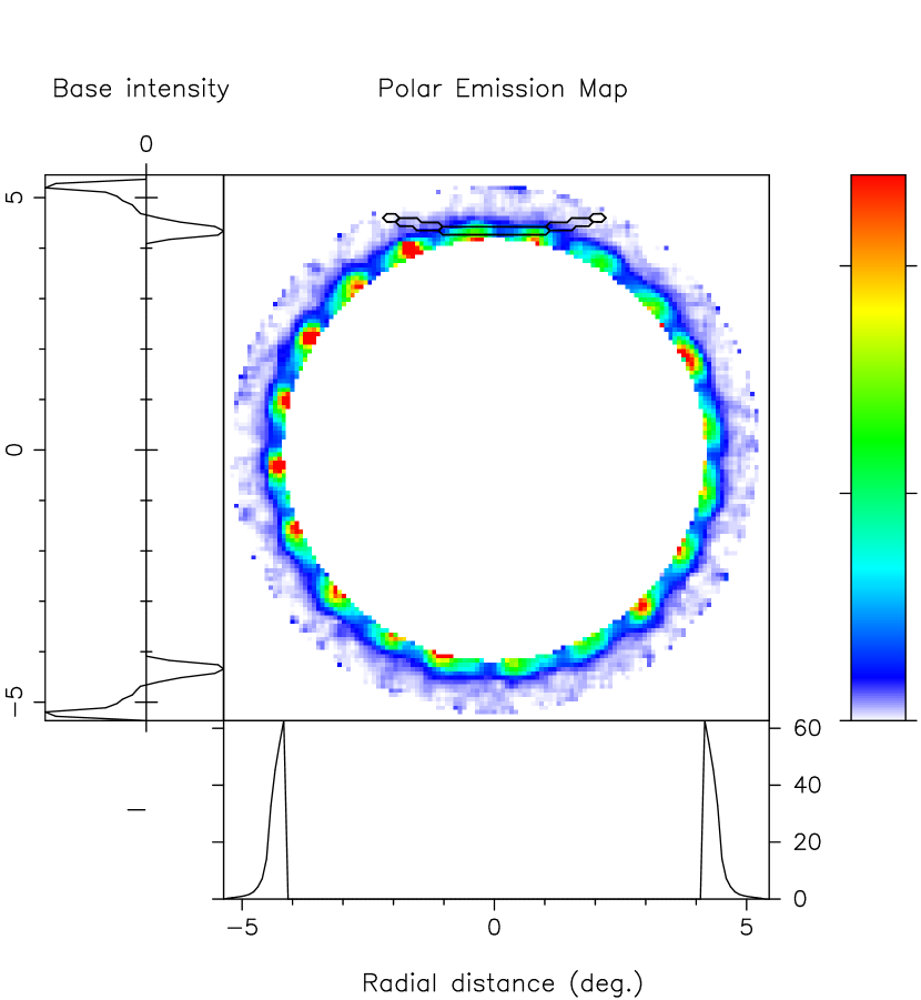
Figure 5: Results of the “cartographic” transformation. The individual-pulse sequence has been mapped onto a rotating frame centred on the magnetic axis. Azimuthal average and minimum (unfluctuating “base”) intensity as a function of magnetic colatitude are given in the bottom and left panels, respectively. Note the twenty emission centres and their somewhat elongated shape. A portion of the sightline traverse is also indicated at the top of the figure.

Applying this cartographic transformation to the “B”-mode portion of our 1992 observations, Figure 5 shows the average configuration of the 20 subbeams which produce the “drift” sequence. The rotation of adjacent beams through our sightline produces the secondary phase modulation, and the periodic pattern of varying beam intensities gives it its tertiary amplitude modulation. We find that the subbeams vary, both in intensity and in azimuthal spacing, over 100-second time scales. Closely spaced beams tend to be weaker, and some beams are observed to bifurcate temporarily, but the 20-fold pattern is always maintained strongly as a stable configuration. The elongated shape of the beams can be understood as a result of truncation, as most of the emission falls inside of the 430-MHz sightline traverse. Indeed, a similar map at a much lower frequency (111.5 MHz), where we expect the sightline to sample emission interior to that one above, shows a more nearly circular subbeam shape.

How sensitive are the conclusions drawn from the cartographic transform to any assumptions in the analysis? The mapping procedure is exquisitely sensitive to the circulation time, and only a little less so to the longitude of the magnetic axis, to the polarisation-angle sweep rate, and to the angles specifying the colatitude of the magnetic axis and sightline “impact” angle. Overall, these parameters scale the map—or utterly distort it. However, the forward transform used to construct the maps has a true inverse transform, and this inverse cartographic transform can be used to “play back” a map in order to produce an artificial pulse sequence. Only when this artificial sequence correlates in full with the observed sequence do we take the map as correct. Indeed, we have carried out such inverse transforms iteratively in a kind of “search mode” to refine each of the requisite parameters, and a completely consistent picture is found in observations from 1974 & 1992 at 430 MHz and from 1990 at 111 MHz.

The overall structure of 0943+10’s radio beam provides new insight into the physical nature of pulsar emission. Its 20 subbeams rotate almost rigidly, maintaining their number and spacing despite perturbations tending both to bifurcate a given beam and to merge adjacent ones—and we find an almost identical subbeam configuration at the two frequencies. These circumstances suggest that the subbeam emission region lies along bundles of magnetic field lines (or “plasma columns”) having “feet” within a certain annulus on the polar cap, wherein charges are accelerated at some distance above the stellar surface and radiation occurs at progressively higher altitudes for lower and lower frequencies. We can thus peer at the activity at the “feet” of the plasma columns and possibly monitor changes viewable at intervals of the circulation time.

The subbeam radiation we observe, estimated to be emitted at some 100-300 km height, then reflects processes occurring at lower altitudes along these ultra-magnetized plasma columns—indeed, some fully down at the surface where the electric fields caused by the star’s rotation appear. The “foot” of each subbeam column moves around the magnetic axis, so we cannot appeal to any surface features or fixed “hot spots” as their cause. The entire rotating-subbeam pattern, averaged over time, represents a hollow-cone beam of emission, which is emitted along the magnetic-field direction at a particular height for a given frequency. Signatures of such conical beams are encountered in most pulsars, and accurately reflect the angular dimension of the magnetic polar cap (Rankin, 1993a).

Nonetheless, we have little guidance about where the “feet” of these plasma columns will fall on the polar cap. Clearly, the radius of the active polar cap $r_{PC}$ scales as the square-root of the star’s radius to that of the light cylinder, $r_{PC}=\epsilon r_{*}(2\pi r_{*}/cP_{1})^{1/2}\sim 145\epsilon P_{1}^{-1/2}$ meters (assuming $r_{*}\approx 10$ km), and values of $\epsilon$ near unity or so have been taken to describe the outside edge of the emission pattern. Therefore, polar-cap features corresponding to the subbeam columns would have separations of some 45$\epsilon$ meters and individual sizes of some 20$\epsilon$ m across. These dimensions would increase only a little even if the “feet” of the plasma columns happen to be a few stellar radii away from the star’s surface. Interpreted another way, our estimate of the angular width of the subbeams (based on the magnetic colatitude spread seen in the map at 111.5 MHz) suggests Lorentz factors $\gamma>200$. We note again that our extremely tangential sightline permits us to sample only the outermost portion of each subbeam at 430 MHz, and so only this outer portion can be mapped down onto the polar cap.

Ruderman & Sutherland (hereafter, R&S), nearly 25 years ago, identified the “drift”-associat-ed subbeams with electrical breakdowns (or “sparks”) in the polar-cap “gap” region, and argued that their circulation was due to E$\times$B drift. Although the major standpoint of their model—that even the enormous electric fields that must be generated would be inadequate to overcome the binding energy of the positive charges (like iron ions) at the neutron-star surface—now seems untenable (Jones, 1985, 1986), closely related models are still in active discussion [e.g., Usov & Melrose (1995); Zhang & Qiao (1996); Zhang (1997)]. It is noteworthy that no completely independent model of subpulse “drift” seems to exist, and our maps do suggest a qualitative picture something like the model R&S envisioned. Any subpulse “drift” model needs to explain first why subpulse-scale structures occur and then why they circulate in azimuth. According to Ferraro’s Theorem (Ferraro & Plumpton, 1966) the open-field region above the polar cap must rotate with, but perhaps more slowly than, the star (so that, for an inertial observer, they would both rotate in the same direction); thus, in the pulsar’s frame the regions will rotate oppositely—as is observed for 0943+10.

Two quantitative features of the R&S model are noteworthy. First, their “gap” height is some 50 m—which is also related in the model to the scale over which an active ”spark” or plasma column inhibits the formation of others—and the 45$\epsilon$ m we infer is fully consistent with this value. Secondly, the observed circulation time can also be reconciled with their model. $\hat{P_{3}}$, at polar-cap radius $r_{s}$, for drifting at velocity $\bf{E}$$\times$$\bf{B}$/$B^{2}$, can be written as $\hat{P_{3}}=2\pi r_{s}B/$$<$$E$$>$$P_{1}$, where $B$ and $<$$E$$>$ are the magnetic field and the average radial electric field in the “gap” region. $<$$E$$>$ in turn depends on the “gap” potential drop $\Delta V$ and the “spark” distance from the edge of the cap, so that the average field is perhaps some $<$$E$$>$$=\Delta V/2(r_{PC}-r_{s})$ [c.f., R&S’s eq.(30)]. Assuming that the pulsar’s magnetic field is correctly computed as a surface value [see de Jager & Nel (1988)’s eq.(1)], then $B$ is 2$\times$10¹² Gauss, $P_{1}$ 1.1 seconds, and thus $\hat{P_{3}}$ can be as large as 37 $P_{1}$ only if $(r_{PC}-r_{s})\sim r_{s}$ and $\Delta V/\epsilon^{2}$ is well less than 10¹² V. In any case, the $<$$E$$>$ in the acceleration region is required to be $\sim 3$$\times$$10^{9}\epsilon$ Volts/meter, for the circulation to be due to E$\times$B drift.

Our maps suggest that the angular velocity associated with the circulation is nearly constant across the radial extent of the subbeams, because no azimuthal shear is observed within the subbeams. The exact origin and significance of any possible dependences of $\hat{P_{3}}$ on radius and other parameters needs to be understood, and similar estimates of circulation time in other pulsars (with different rotational parameters and geometries) should help to define this issue. The finely-tuned stability of the pattern observed in this pulsar has more to tell. It is unlikely that the remarkably periodic and stable arrangement would be possible if the required spacing of subbeams were not an integral submultiple of the circumference of the ring on which they appear to arrange themselves. Pulsar B0943+10’s particular characteristics may therefore result from a critical combination of parameters—namely, its rotation period, emission geometry, magnetic field strength and subbeam spacing, which in turn could be determined by the “gap” height. It should not, therefore, be surprising to find that this remarkable configuration is indeed an unusual one.

Nevertheless, averaged over many circulation times, 0943+10’s emission pattern conclusively demonstrates the existence of the hollow-conical emission beams long attributed to many pulsars through less direct means. The subbeam columns must be nearly axially symmetric with respect to the magnetic axis, because any significant deviation would require a contrived situation to reproduce the periodicities and polarization that we observe. Models in which only a part of the polar cap is active [e.g., Arons & Scharlemann (1979); Arons (1979)] are incompatible with these results.

The central conclusion to be drawn from our subbeam mapping of pulsar B0943+10 is that the emitting pattern—which is so very stable over hundreds of seconds or many circulation cycles—is frozen neither to the fields nor to the stellar surface. We must then ask where, physically, the “memory” of the subbeam pattern is carried in this system of charges and particle currents despite the circulation. The detailed structure that we have mapped traces the activity at the “feet” of the emission columns and represents the first direct measurements of some of the parameters—such as the locations, size and movement of the underlying pattern—reflecting the electrodynamics not very far from the stellar surface. The overall continuity of the emission, implicit in the stability of the pattern over many circulation periods, demands a remarkable “collective steadiness” at every stage of the emission process—such as, generation and acceleration of particles and coherent amplification.

In summary, pulsar 0943+10 exhibits an exqui-sitely stable “drifting”-subpulse pattern in its “B” mode sequences with a nearly even-odd fluctuation frequency of about 0.53 c/$P_{1}$. Upon first establishing the aliasing-order of this feature, and then accurately modeling the star’s emission geometry, the two “sideband” features were found to result from a tertiary amplitude modulation on the secondary phase modulation. The remarkable precision of the modulation rates argues for a system of subbeams circulating around the magnetic axis, prompting the use of a novel “cartographic” transform to map the subbeam structure responsible for the pulse-to-pulse fluctuations. The detailed parameters of the circulating subbeams allow quantitative assessment of the possible interpretation in terms of the system of rotating “sparks” on the polar cap as suggested in the Ruderman & Sutherland model. The current analysis holds considerable promise for studying the emission properties in other pulsars and for assessing physical emission theories.

Figure 1: A series of individual pulses from pulsar B0943+10 (centre panel) along with their average (bottom panel) and energy (left panel) as a function of pulse number and longitude (360^o longitude correspond to one stellar rotation). Note the “drifting” subpulses, the alternate-pulse modulation, and the “single” average profile.

Figure 2: Fluctuation-spectral power (centre panel) as a function of longitude and frequency as well as the integral spectrum (bottom panel). Note the primary and secondary features at about 0.46 and 0.07 cycles/period as well as the symmetrical “sidebands” around the former.

Figure 3: Fluctuation spectrum of a continuously-sampled time sequence reconstructed from the (gated) single-pulse sequence used in Fig. 2. The spectrum is presented in a matrix form with each row showing a section of the spectrum between $n/P_{1}$ to $(n+1)/P_{1}$ for harmonics $n=0,1,2,...$ of the rotation frequency $1/P_{1}$. The harmonics at $n/P_{1}$ are shown separately (left panel) and are essentially the Fourier components of the average profile. All other frequency components (up to $100/P_{1}$) are given as a contour plot (centre panel), and the column sum of these components, collapsed into a $1/P_{1}$ interval (bottom panel), can be compared directly with Fig. 2. Note that the principal feature now falls at an (unaliased) frequency of about 0.535 c/$P_{1}$. Note also that whereas the Fourier amplitudes of the principal feature peak at about harmonic (row) number 35 (corresponding to a $P_{2}$ value of some $10.5^{o}$), those of the secondary feature peak around number 70—thus demonstrating their harmonicity.

Figure 4: Pulse sequence folded at the full 37.35-period modulation cycle (centre panel). Twenty emission centres can be readily identified, and their relative intensity is shown as a function of longitude (bottom panel) and modulation phase in units of pulse number (left panel). For comparison, the dots in the latter show the result using a tertiary period that is 2% different than the correct one.

References

- Arons (1979) Arons, J. 1979, Space Sci. Rev., 24, 437
- Arons & Scharlemann (1979) Arons, J. & Scharlemann, E. T. 1979, ApJ, 231, 854
- Backer (1973) Backer, D. C 1973, ApJ, 182, 245
- Backer et al. (1975) Backer, D. C., Rankin, J. M., & Campbell, D. B. 1975, ApJ, 197, 481
- Deshpande & Rankin (1999) Deshpande, A. A. & Rankin, J. M. 1999, in preparation.
- Drake & Craft (1968) Drake, F. D., & Craft, H. D. jr 1968, Nature, 220, 231
- Ferraro & Plumpton (1966) Ferraro, V. C. A., & Plumpton, C. 1966, Magneto-Fluid Mechanics (London: Oxford University Press), 23.
- de Jager & Nel (1988) de Jager, O. C., & Nel, H. I. 1988, A&A, 190, 87
- Jones (1985) Jones, P. B. 1985, Phys. Rev. Lett., 55, 1338
- Jones (1986) Jones, P. B. 1986, MNRAS, 218, 477
- Manchester et al. (1975) Manchester, R. N., Taylor, J. H., & Huguenin, G. R. 1975, ApJ, 196, 83
- Mitra & Deshpande (1999) Mitra, D., & Deshpande, A. A. 1999, A&A, preprint
- Radhakrishnan & Cooke (1969) Radhakrishnan, V., & Cooke, D. J. 1969, Astrophys. Lett., 3, 225
- Rankin (1990) Rankin, J. M. 1990, ApJ, 352, 247
- Rankin (1993a) Rankin, J. M. 1993a, ApJ, 405, 285
- Rankin (1993b) Rankin, J. M. 1993b, ApJS, 85, 145
- Ruderman & Sutherland (1975) Ruderman, M. A., & Sutherland, P. G. 1975, ApJ, 196, 51
- Ruderman (1976) Ruderman, M. A. 1976, ApJ, 203, 206
- Sieber & Oster (1975) Sieber, W., & Oster, L. 1975, A&A, 38, 325
- Sieber & Oster (1976) Sieber, W., & Oster, L. 1976, ApJ, 210, 220
- Suleymanova & Izvekova (1984) Suleymanova, S. A., & Izvekova, V. A. 1984, Soviet Astronomy, 28, 32
- Suleymanova et al. (1998) Suleymanova, S. A., Izvekova, V. A., Rankin, J. M. & Rathnasree, N. 1998, J. Astrophys. Astron., 19, 1
- Taylor & Cordes (1993) Taylor, J. H. & Cordes, J. M. 1993, ApJ, 401, 674
- Taylor & Huguenin (1971) Taylor, J. H., & Huguenin, G. R. 1971, ApJ, 167, 273
- Taylor et al. (1971) Taylor, J. H., Huguenin, G. R., Hirsch, R. M., & Manchester, R. N. 1971, Astrophys. Lett., 9, 205
- Taylor et al. (1993) Taylor, J. H., Manchester, R. N., & Lyne, A. G. 1993, ApJS, 88, 529
- Usov & Melrose (1995) Usov, V. V., & Melrose, D. B. 1995, Australian J Phys., 48, 571
- Vitkevich, et al. (1969) Vitkevich, V. V., Alexseev, Yu. I., & Zhuravlev, Yu. P. 1969, Nature, 224, 49
- Zhang & Qiao (1996) Zhang, B., & Qiao, G. J. 1996, A&A, 310, 135
- Zhang (1997) Zhang, B. 1997, ApJ, 478, 313