Caltech Faint Field Galaxy Redshift Survey IX:
Source Detection and Photometry in the Hubble Deep Field Region

Abstract

Detection and photometry of sources in the $U_{n}$, $G$, $\cal R$, and $K_{s}$ bands in a $9\times 9$ arcmin² region of the sky, centered on the Hubble Deep Field, are described. The data permit construction of complete photometric catalogs to roughly $U_{n}=25$, $G=26$, ${\cal R}=25.5$ and $K_{s}=20$ mag, and significant photometric measurements somewhat fainter. The galaxy number density is $1.3\times 10^{5}~{}{\rm deg^{-2}}$ to ${\cal R}=25.0$ mag. Galaxy number counts have slopes $d\log N/dm=0.42$, $0.33$, $0.27$ and $0.31$ in the $U_{n}$, $G$, $\cal R$ and $K_{s}$ bands, consistent with previous studies and the trend that fainter galaxies are, on average, bluer. Galaxy catalogs selected in the $\cal R$ and $K_{s}$ bands are presented, containing 3607 and 488 sources, in field areas of $74.8$ and $59.4~{}{\rm arcmin^{2}}$, to ${\cal R}=25.5$ and and $K_{s}=20$ mag.

1 Introduction

The Hubble Deep Field (HDF, Williams et al 1996) was chosen to be at high Galactic latitude, at low extinction, and free of bright or unusual sources. The Hubble Space Telescope (HST) images of the HDF are the deepest optical images of the sky ever taken, reaching source densities of roughly $10^{6}~{}{\rm deg^{-2}}$. The HDF has quickly become a “standard field” for the study of very faint extragalactic sources; it has been studied at all wavelengths from x-ray to radio. It is hoped that the huge multi-wavelength database which is developing for this field will lead to a new understanding of faint galaxy properties and evolution. In this paper are presented the catalogs of source fluxes and colors created for the Caltech Faint Galaxy Redshift Survey, in a region of the sky centered on the the HDF.

The Caltech Faint Galaxy Redshift Survey is a set of magnitude-limited visual spectroscopic surveys, with visual- and near-infrared-selected samples of very faint sources in blank fields. The sources are observed spectroscopically with the Low Resolution Imaging Spectrograph (LRIS, Oke et al 1995) instrument on the Keck Telescope. The spectroscopic catalogs are presented in companion papers (Cohen et al 1999a, Cohen et al 1999c). Briefly, the survey comprises several fields which together contain many hundreds of sources with spectroscopically measured redshifts and multi-band photometry, down to $R\approx 24.5$ or $K\approx 20$ mag, the current practical limit of highly complete, magnitude-limited spectroscopic samples. (Of course the photometric catalogs, and some incomplete spectroscopic samples, reach fainter fluxes than these.) Early results include studies of galaxy groups out to redshifts $z\approx 1$ (Cohen et al 1996a, 1996b, 1999b, 1999c) and measurements of broad-band and emission line luminosity functions and their evolution to redshifts $z\approx 1.5$ (Hogg et al 1998a; Hogg 1998b; Cohen et al 1999b). The database of photometry and spectroscopy will be useful for studies of faint galaxies and stars.

The HST images of the HDF are very small, covering only about 5 arcmin², so they are poorly matched to the 15 arcmin² spectroscopic field of the LRIS instrument. For this reason the spectroscopic surveys in the HDF are performed in a larger region of the sky surrounding the HST image, with sources selected with the ground-based data presented here. The HDF observations with HST also included short exposures (one or two orbits) for eight pointings surrounding the HDF; these are referred to as the “Flanking Fields” (FF). The potential for obtaining detailed morphological information on the brighter sources at the resolution of HST therefore exists for the photometric catalogs presented here, and the redshift catalogs presented elsewhere (Cohen et al 1996a, 1996b, 1999c).

2 Data

For visual data, $U_{n}$, $G$ and $\cal R$ images taken with the COSMIC camera (Kells et al 1998) at the prime focus of the 200-inch Hale Telescope at the Palomar Observatory were used. The COSMIC camera has $0.283\times 0.283~{}{\rm arcsec^{2}}$ pixels over a $9\times 9~{}{\rm arcmin^{2}}$ field of view. The final, stacked images images are $8.6\times 8.7~{}{\rm arcmin^{2}}$, centered on 12 36 51.4 +62 13 13 (J2000), ie, roughly centered on the HST image of the HDF (Williams et al 1996). The visual images were taken in order to identify candidate $z>3$ galaxies; details of the observations, calibration, and reduction of these images are described in Steidel et al (in preparation). The $U_{n}$, $G$ and $\cal R$ filters are described in Steidel & Hamilton (1993); briefly, they have effective wavelengths of 3570, 4830 and 6930 Å, FWHM bandpasses of 700, 1200 and 1500 Å, and zero-magnitude flux densities of roughly 1550, 3890 and 2750 Jy. These magnitudes are Vega-relative, not AB.

The southwest corner of the $\cal R$ image was contaminated by an asteroid trail. The trail was removed by transforming less sensitive but higher-resolution Keck LRIS $R$-band images taken as set-up for the spectroscopic program in this field (Cohen et al 1999c) onto the same pixel scale, smoothing to the same seeing, and scaling to the same zeropoint. A strip of full width $4.7~{}{\rm arcsec}$ along the straight trail was replaced with the smoothed, transformed Keck LRIS image. This thin strip of the $\cal R$-band image has slightly higher-than-average noise.

For near-infrared data, an 8-arcmin diameter circular region centered on the HDF was imaged on 1997 March 19–21 using a $K_{s}$ filter with a near-infrared camera (Jarrett et al 1994) mounted at the prime focus of the 200-inch Hale Telescope. The instrument reimages the focal plane at 1:1 onto a NICMOS–3 $256\times 256~{}{\rm pixel}$ HgCdTe array (produced by Rockwell), producing a $0.494\times 0.494~{}{\rm arcsec^{2}}$ projected pixel size and a $2.1\times 2.1~{}{\rm arcmin^{2}}$ instantaneous field of view. The $K_{s}$ filter has an effective wavelength of $2.15~{}{\rm\mu m}$, a FWHM bandpass of $0.3~{}{\rm\mu m}$, and a zero-magnitude flux density of roughly 708 Jy. Fourteen separate subfields, offset by 2 arcmin, were required in order to mosaic the entire circular field; each of these subfield was imaged once per night. For each subfield each night, 45 separate frames were taken; each frame consisted of six exposures of three seconds each, coadded in the electronics before writing to disk. The telescope was dithered by 5–15 arcsec between frames. As a result, each subfield was exposed for 810 s each night, or 2430 s for the three nights. The seeing was $\sim 1.0$ arcsec FWHM for most of the three nights. The first two nights were judged photometric, and were calibrated using the faint Solar-type standard stars of Persson et al (1998).

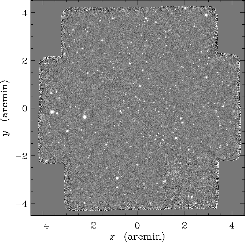
Figure 2: The final $K_{s}$–band mosaic, stretched from $-5\,\sigma$ (black) to $5\,\sigma$ (white).

The $K_{s}$-band data were reduced by the method of Pahre et al (1997). Each subfield was reduced separately for each night. The third night’s data were rescaled by factors of between 1.1 and 1.5 in order to account for cirrus; the scaling factors were determined from a fit to a large number of sources. The subfields were then registered by aligning the objects in common with adjacent subfields in the overlap region. Individual pixels in a given field were weighted by the number of pointings contributing to that pixel. A background level was estimated at every pixel by median-filtering the mosaic with a wide filter and sigma–clipping. This background was subtracted in order to remove subfield-to-subfield variations in the sky brightness of the final mosaic. The final $K_{s}$–band mosaic is displayed in Figure 2.

Table 1 gives the properties of the final, stacked images.

3 Source detection

Sources were detected in all four images independently to construct four catalogs, hereafter “$U_{n}$-selected”, “$G$-selected”, “$\cal R$-selected” and “$K_{s}$-selected”. All catalogs were created with the SExtractor source detection and photometry package (Bertin & Arnouts 1996). The detection algorithm is as follows: Images are smoothed with a Gaussian filter which has roughly the same FWHM as the seeing (1.13 arcsec for the visual images and 1.5 arcsec for the $K_{s}$-band image). Sources in the smoothed image with central-pixel surface brightness above a certain limit are added to the catalog. If a source has multiple peaks within its 1.2-$\sigma$ isophotal area on the image (where $\sigma$ is the pixel-to-pixel root-mean-square fluctuation in the sky brightness), each peak is split into a separate catalog source if it contains at least one percent of the original source’s isophotal flux.

The $\cal R$-selected SExtractor catalog was augmented in two ways. (1) Several sources were added which, by eye, appear that they ought to be split off of brighter nearby objects but were not. These sources, when above the $\cal R$-band flux limit, were added to the $\cal R$-selected catalog directly. (2) Several very faint sources were compiled into what is hereafter the “supplemental” catalog, even though they are below the $\cal R$-selected catalog’s flux limit, because they have successful redshift measurements in the companion paper Cohen et al (1999c). The fluxes for the supplemental catalog are all aperture magnitudes and the colors were measured as described below.

The noise in the $K_{s}$ image is much worse along the edges of the mosaic than at the center, which can lead to spurious detections. Sources in the high-noise edges were removed from the $K_{s}$-selected catalog, leaving a total area coverage of $59.4~{}{\rm arcmin^{2}}$.

4 Calibration with HST imaging

To maintain a flux or magnitude system consistent with previous work in the HDF, the $U_{n}$, $G$ and $\cal R$ images are calibrated by comparison with the extremely deep HST images of the HDF. The acquisition, reduction and calibration of the HST images are described in Williams et al (1996). In what folows, the Vega-relative calibrations of the HST images are used.

The absolute calibrations and effective wavelengths for the HST and ground-based filters are used to compute the following transformation equations under the assumption that the sources have roughly power-law spectral energy distributions:

$$U_{n}=0.53\,F300W+0.47\,F450W-0.29~{}{\rm mag}$$ (1)

$$G=0.82\,F450W+0.18\,F606W-0.07~{}{\rm mag}$$ (2)

$${\cal R}=0.46\,F606W+0.54\,F814W-0.02~{}{\rm mag}$$ (3)

where $F300W$, $F450W$, $F606W$ and $F814W$ are Vega-relative magnitudes in the HST bandpasses of the same name.

The “Version 2” HST HDF images (Williams et al 1996) are transformed onto the $U_{n}$, $G$ and $\cal R$ image coordinate system and all seven images are Gaussian-smoothed to have the same effective seeing. Aperture magnitudes were measured for the $\cal R$-selected sample through matched, 2-arcsec diameter apertures. For calibration, the Vega-relative magnitude zeropoints were used instead of the “AB” zeropoints used by Williams et al (1996). The measured $U_{n}$, $G$ and $\cal R$-band magnitudes are given zeropoints such that the comparison with transformed HST magnitudes in Figure 3 shows the best possible agreement. This HST-relative calibration ought to be good to roughly 5 percent.

5 Photometry

All catalog sources were photometered two ways: Isophotal magnitudes were measured down to the 2-$\sigma$ isophote (where $\sigma$ is the pixel-to-pixel root-mean-square fluctuation in the sky brightness). Aperture magnitudes were measured through apertures of diameter 1.7 arcsec for the visual images and 2.0 arcsec for the $K_{s}$-band image. Corrections to account for flux outside the aperture were added to the raw aperture magnitudes. The aperture corrections were measured from bright stars in the field and were found to be $-0.13$, $-0.10$, $-0.10$ and $-0.12$ mag for the $U_{n}$, $G$, $\cal R$ and $K_{s}$ images respectively. These corrections correct aperture magnitudes to total magnitudes for point sources; no adjustment was made to account for galaxy size or extended structure in galaxies because although faint galaxies are not point sources, in these ground-based images there is almost no detectable difference between a faint galaxy and star at the faintest levels. Each source in the catalogs was assigned a “total magnitude” which is the brighter of the isophotal and corrected-aperture magnitudes. In practice, this is the isophotal magnitude for $79.9$ percent of sources to ${\cal R}=24.5$ mag, and it is $42.5$ percent to ${\cal R}=25.5$ mag; and it is $98.5$ percent to $K_{s}=19$ mag and $71.9$ percent to $K_{s}=20$ mag. It should be noted that under this definition, the total magnitudes are not expected to represent entire source fluxes, because there may be significant flux at large radius and low surface-brightness around these sources. Unfortunately it is not possible to accurately measure this low surface-brightness flux on a source-by-source basis.

6 Color measurement

To measure unbiased colors, the visual images were smoothed with Gaussians to the same effective seeing as the $K_{s}$-band image. A catalog of over 500 objects common to the visual and $K_{s}$-band images were used to derive the fourth-order polynomial transformation mapping the visual images onto the $K_{s}$-band image and vice versa (with NOAO/IRAF tasks “geomap” and “geotran”). Colors were measured through matched apertures of diameter 2 arcsec. For the $U_{n}$, $G$ and $\cal R$-selected catalogs, colors were measured in the smoothed visual image and the $K_{s}$-band image transformed onto the visual coordinates. For the $K_{s}$-selected catalog, colors were measured in the smoothed visual images transformed onto the $K_{s}$-band image coordinates and the $K_{s}$-band image.

Color distributions for the four main catalogs are shown in Figures 4 through 7. There are 1920 sources with $U_{n}<25.0$ mag in the $U_{n}$-selected catalog, 2863 with $G<26.0$ mag in the $G$-selected, 3607 with ${\cal R}<25.5$ mag in the $\cal R$-selected, and 488 with $K_{s}<20.0$ mag in the $K_{s}$-selected. The full $\cal R$-selected, $K_{s}$-selected, and supplemental catalogs are given in Tables 2, 3, and 4. [For now the tables are available at
(http://www.sns.ias.edu/~hogg/Hogg.Rsel.txt), (http://www.sns.ias.edu/~hogg/Hogg.Ksel.txt), and (http://www.sns.ias.edu/~hogg/Hogg.extras.txt).]

7 Astrometry

Absolute positions were assigned to the $\cal R$-selected sources by comparison with the Williams et al (1996) and Phillips et al (1997) catalogs. In the HST-imaged portion of the field, absolute positions were found by identifying $\cal R$-selected sources with those in the Williams et al catalog. In the flanking field, the $\sim 100$ sources in the Phillips et al catalog were identified with $\cal R$-selected sources. A quadratic transformation was fit to the relation between COSMIC pixel locations and absolute positions for the identified sources. This transformation was used to assign absolute positions to all sources in the $\cal R$-selected catalog. These positions are given in Tables 2, 3, and 4. Comparison with the radio maps of the HDF and flanking fields (Richards et al 1998) shows that the absolute positions have an rms accuracy of roughly 0.4 arcsec (Cohen et al 1999c).

8 Completeness

It appears from Figures 4 through 7 that the catalogs are complete to roughly $U_{n}=25$, $G=26$, ${\cal R}=25.5$ and and $K_{s}=20$ mag. No completeness simulations have been performed because the primary purpose of this study is to construct catalogs for spectroscopy, not to measure ultra-deep number counts. For the latter study, better data exist and have been analyzed. With typical colors, objects with ${\cal R}>24$ mag and $K_{s}>20$ mag cannot routinely, or with good completeness, be measured spectroscopically with the Keck Telescope, so this catalog is appropriate for selection of a complete spectroscopic sample.

9 Discussion

The results of this survey are entirely contained in Figures 4 through 7. However, they can be compared with the results of other authors. When divided by the solid angle of the $8.6\times 8.7~{}{\rm arcmin^{2}}$ field, the integrated number of sources is $1.3\times 10^{5}~{}{\rm deg^{-2}}$ to ${\cal R}=25.0$ mag. This is consistent with number counts from similar studies (eg, Hogg et al 1997b). The color distributions are also consistent with the results of previous studies, in mean and scatter (Hogg et al 1997a, 1997b; Pahre et al 1997).

Number–flux relations of the power-law form $d\log N/dm=Q$, where $Q$ is a constant, can be fit to the $U_{n}$, $G$ and $\cal R$-selected catalogs over the 4-magnitude range terminating at the completeness limits given in Section 8. In the $K_{s}$-selected catalog the fit is performed only over $18<K<20$ mag because many studies have shown that the slope changes significantly at $K\approx 18$ mag (eg, Gardner et al 1993; Djorgovski et al 1995). The resulting faint-end slopes are $Q=0.42$, $0.33$, $0.27$ and $0.31$ for the $U_{n}$, $G$, $\cal R$ and $K_{s}$ counts respsectively. These slopes are consistent with those found in previous studies (Djorgovski et al 1995; Metcalfe et al 1995; Hogg et al 1997b; Pahre et al 1997).

Although all these observations are consistent with the results of previous observational studies, the bulk of the faint sources are significantly bluer than normal, bright galaxies would be if there were no evolution in galaxy spectra. For example, a non-evolving spiral galaxy would have ${\cal R}-K_{s}\approx 3$ mag at redshift $z=0.6$, and the bluest local galaxies would have ${\cal R}-K_{s}\approx 2.5$ mag, but in the samples presented here, where the median redshift is roughly 0.6 (Cohen et al 1999a, 1999c), there are many galaxies with ${\cal R}-K_{s}<2$ mag. The appearance of this extremely blue population in faint samples is a consequence of the high star formation rates at intermediate and high redshift relative to those of in the present-day Universe, as inferred from metallicity in Lyman-alpha clouds (Pei & Fall 1995), ultraviolet luminosity density (Lilly et al 1996; Connolly et al 1997; Madau et al 1998) and emission line strengths (Hammer et al 1997; Heyl et al 1997; Small et al 1997; Hogg et al 1998). This evolutionary effect, the decrease in star formation rate since redshift unity, is perhaps the most widely and independently confirmed result in the study of field galaxy evolution.

Table 1: Imaging data parameters, for final, stacked mosaics

band	solid angle	exposure	pixel size	seeing FWHM	$1\,\sigma$ in aperture
	(arcmin2)	(s)	(arcsec)	(arcsec)	(mag)
$U_{n}$	75	23400	0.283	1.3	26.9
$G$	75	7200	0.283	1.2	28.1
$\cal R$	75	6000	0.283	1.1	27.2
$K_{s}$	59	2430	0.494	1.5	22.1

Table 2: The $\cal R$-selected catalog

Table 3: The $K_{s}$-selected catalog

Table 4: The supplemental catalog

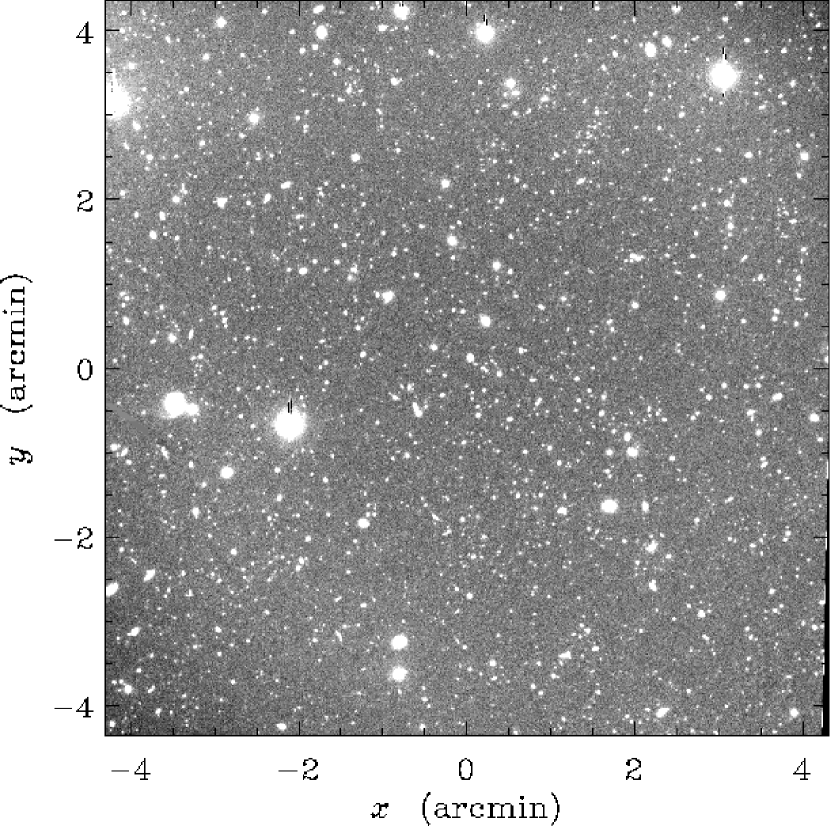
Figure 1: The final $\cal R$–band mosaic, stretched from $-5\,\sigma$ (black) to $5\,\sigma$ (white). The field center is 12 36 51.4 +62 13 13 (J2000).

Figure 3: Comparison of ground-based visual and transformed HST magnitudes for the $\cal R$-selected sample. These plots were used to calibrate the $U_{n}$, $G$ and $\cal R$ images.

Figure 4: Number counts of $U_{n}$-selected sources and their colors. The number counts have not been corrected for incompleteness, which appears to set in at $U_{n}\approx 25$ mag.

Figure 5: Number counts of $G$-selected sources and their colors. The number counts have not been corrected for incompleteness, which appears to set in at $G\approx 26$ mag.

Figure 6: Number counts of $\cal R$-selected sources and their colors. The number counts have not been corrected for incompleteness, which appears to set in at ${\cal R}\approx 25.5$ mag.

Figure 7: Number counts of $K_{s}$-selected sources and their colors. The number counts have not been corrected for incompleteness, which appears to set in at $K_{s}\approx 20$ mag.

References

- (1) Bertin E., Arnouts S., 1996, A&AS 117 393
- (2) Cohen J. G., Hogg D. W., Pahre M. A. & Blandford R., 1996a, ApJ 462 L9
- (3) Cohen J. G., Cowie L. L., Hogg D. W., Songaila A., Blandford R., Hu E. M. & Shopbell P., 1996b, ApJ 471 L5
- (4) Cohen J. G., Hogg D. W., Pahre M. A., Blandford R., Shopbell P. & Richberg K., 1999a, ApJS 120 171
- (5) Cohen J. G., Blandford R., Hogg D. W., Pahre M. A. & Shopbell P. L., 1999b, ApJ 512 30
- (6) Cohen J. G., Hogg D. W., Blandford R., Cowie L. L., Hu E., Songaila A., Shopbell P. & Richberg K., 1999c, ApJ submitted
- (7) Connolly A. J., Szalay A. S., Dickinson M., Subbarao M. U. & Brunner R. J., 1997, ApJ 486 L11
- (8) Djorgovski S. et al, 1995, ApJ 438 L13
- (9) Gardner J. P., Cowie L. L. & Wainscoat R. J., 1993, ApJ 415 L9
- (10) Hammer F., Flores H., Lilly S. J., Crampton D., Le Fèvre O., Rola C., Mallen-Ornelas G., Schade D. & Tresse L., 1997, ApJ 481 49
- (11) Heyl J., Colless M., Ellis R. S. & Broadhurst T., 1997, MNRAS 285 613
- (12) Hogg D. W., Neugebauer G., Armus L., Matthews K., Pahre M. A., Soifer B. T. & Weinberger A. J., 1997a, AJ 113 474 (erratum AJ 113 2338)
- (13) Hogg D. W., Pahre M. A., McCarthy J. K., Cohen J. G., Blandford R. D., Smail I. & Soifer B. T., 1997b, MNRAS 288 404
- (14) Hogg D. W., Cohen J. G., Blandford R. & Pahre M. A., 1998a, ApJ 504 622
- (15) Hogg D. W., 1998b, PhD thesis, Caltech
- (16) Jarrett T. H., Beichman C., Van Buren D., Gautier N. & Bruce C., 1994, in Infrared Astronomy with Arrays: The Next Generation, ed. McLean I., Kluwer, Dordrecht, 293
- (17) Kells W., Dressler A., Sivaramakrishnan A., Carr D., Koch E., Epps H., Hilyard D. & Pardeilhan G., 1998, PASP 110 1487
- (18) Lilly S. J., Le Fèvre O., Hammer F. & Crampton D., 1996, ApJ 460 L1
- (19) Madau P., Pozzetti L. & Dickinson M., 1998, ApJ 498 106
- (20) Metcalfe N., Shanks T., Fong R. & Roche N., 1995, MNRAS 273 257
- (21) Oke J. B., Cohen J. G., Carr M., Cromer J., Dingizian A., Harris F. H., Labrecque S., Lucinio R., Schaal W., Epps H. & Miller J., 1995, PASP 107 375
- (22) Pahre M. A. et al, 1997, ApJS submitted
- (23) Pei Y. C. & Fall S. M., 1995, ApJ 454 69
- (24) Persson S. E., Murphy D. C., Krzeminski W., Roth M. & Rieke, M., 1998, AJ 116 2475
- (25) Phillips A. C., Guzman R., Gallego J., Koo D. C., Lowenthal J. D., Vogt N. P., Faber S. M. & Illingworth G. D., 1997, ApJ 489 543
- (26) Richards E. A., Kellerman K. I., Fomalont E. B., Windhorst R. A. & Partridge R. B., 1998, AJ 116 1039
- (27) Small R. A., Sargent W. L. W. & Hamilton D., 1997, ApJ 487 512
- (28) Steidel C. C. & Hamilton D., 1993, AJ 105 2017
- (29) Williams R. E. et al, 1996, AJ 112 1335