Magnetosphere of Oscillating Neutron Star. Nonvacuum Treatment.

Abstract

We generalize a formula for the Goldreich-Julian charge density ($\rho_{\mbox{\tiny GJ}}$), originally derived for rotating neutron star, for arbitrary oscillations of a neutron star with arbitrary magnetic field configuration under assumption of low current density in the inner parts of the magnetosphere. As an application we consider toroidal oscillation of a neutron star with dipole magnetic field and calculate energy losses. For some oscillation modes the longitudinal electric field can not be canceled by putting charged particles in the magnetosphere without a presence of strong electric current ($j\simeq\frac{c}{\omega r}\,\rho_{\mbox{\tiny GJ}}\>c$). It is shown that the energy losses are strongly affected by plasma in the magnetosphere, and cannot be described by vacuum formulas.

1 Introduction

Oscillations of neutron stars could give an opportunity to study their internal structure. Oscillations of a neutron star (NS) may be observable in pulsars just after a glitch. The energy release during the glitch is estimated as

$$E\sim\frac{1}{2}\frac{M_{\mbox{\tiny crust}}}{M_{\mbox{\tiny NS}}}I\Omega^{2}\frac{\Delta\Omega}{\Omega}\>,$$ (1)

where $I$ is the moment of inertia of the NS, $\Omega$ is an angular velocity of rotation, $\Delta\Omega$ is a jump of angular velocity, $M_{\mbox{NS}}$ is a mass of the NS, $M_{\mbox{crust}}$ is a mass of the crust. For the Vela pulsar $E\sim 10^{37}$ergs. There are about 20 glitching pulsars, which had suffered a total of 45 glitches [1996]. The energy release in each of these glitches is similar to that of the Vela pulsar. If several percent of this energy goes into excitation of oscillations it would be possible to observe them. Another example how oscillations of NS could be observed in pulsars is by observations of microstructure in single pulses. Boriakoff [1976] proposed that vibrations of a neutron star may cause the periodicity of micropulses observed in some pulsars. A difficulty in this theory is that no effective mechanism has been proposed for excitation of oscillations [1996].

Oscillating neutron stars have been proposed as a source for Galactic Gamma-Ray Bursts (GRBs) by Pachini & Ruderman [1974] and Tsygan [1975]. This idea is further developed by Blaes et al. [1989], Smith & Epstein [1993], Fatuzzo & Melia [1993]. Oscillation induced hard gamma radiation from NS was proposed by Bisnovatyi-Kogan [1995] and Cheng & Ding [1997] for explanation of the hard delayed emission observed from some GRBs [1994], even if the Gamma-Ray Burst itself is generated by a different mechanism [1975]. Recent GRBs observations make a Galactic origin of GRBs unlikely, but a Galactic model may not be excluded completely. At least for Soft Gamma Repeaters, which are believed to be neutron stars, oscillations of star can play an essential role (Duncan 1998).

Eigenfrequencies and eigenfunctions of neutron star oscillations have been computed by many authors [1988, 1986, 1991]. These calculations have shown that typical periods of neutron star oscillations range from $0.1$ up to several tens of milliseconds. On the other hand, observed pulsar radiation in different spectral regions is generated mostly in their magnetospheres [1998]. If we are looking for oscillation induced radiation from pulsars we should investigate processes in the magnetosphere. A complete solution for vacuum electromagnetic fields near an oscillating magnetized neutron star was obtained by Muslimov and Tsygan [1986]. But for typical NS’s magnetic field strength ($>10^{9}$G) the electric field arising from star‘s oscillation will be strong enough to pull charged particles from the surface in the magnetosphere. Hence, any realistic model of the magnetosphere of oscillating NS must take into account the presence of charged particles. This will also affect the electromagnetic energy losses of a pulsating magnetized star. Electromagnetic energy losses of an oscillating NS in vacuum were calculated by McDermott at al. [1984] and Muslimov and Tsygan [1986]

As a first step in the investigation of magnetosphere of an oscillating neutron star with nonzero charge density we consider the inner part of the magnetosphere, assuming low current density there. We generalize a formula for Goldreich-Julian charge density, derived originally for rotating NS, for a NS oscillating in any arbitrary mode. This allow us to take into account plasma present in the magnetosphere of the NS and calculate the energy losses. The plan of the paper is following. In the first section we introduce some definitions and give algorithm for calculation of Goldreich-Julian charge density for arbitrary oscillation mode and magnetic field structure under the assumption of low current density, and discuss the limitations of this assumption. In the second section we apply this formalism to toroidal oscillations of a NS with a dipole magnetic field. We calculate the Goldreich-Julian charge density and energy losses for some oscillation modes and discuss factors affecting energy losses of oscillating neutron star.

2 Goldreich-Julian charge density for small amplitude oscillations of a neutron star. General formalism.

2.1 Basic definitions.

As it was firstly pointed by Goldreich and Julian [1969] a rotating NS can not be surrounded by vacuum. The electric field generated by rotation of magnetized NS will pull charged particles into the magnetosphere – the electrostatic force near the NS’s surface in vacuum would be much stronger than the gravitational one for both electrons and ions. According to the calculations of Jones [1986], the binding of charged particles in the crust of a typical pulsar is not strong enough to prevent them being pulled into the magnetosphere by the vacuum electric field. But even if the binding of charged particles in the cold crust of an old NS can prevent them escaping, the magnetosphere of a strong magnetized neutron star can be filled by charged particles by the mechanism proposed by Ruderman and Sutherland [1975] for pulsars.

On the NS surface the vacuum electric field generated by rotation or oscillation has a radial component, whose value is a substantional part of the full field strength [1986, 1969]. To order of magnitude this field for the rotating star is

$$E^{\rm rot}\simeq\frac{\Omega r_{*}}{c}B\ ,$$ (2)

where $\Omega$ is the rotational frequency of the NS, $r_{*}$ is NS radius and $B$ is the magnetic field strength near the star. In the case of NS oscillations the corresponding vacuum electric field is

$$E^{\rm osc}\simeq\frac{\omega\xi}{c}B\ ,$$ (3)

where $\omega$ is the oscillation frequency, $\xi$ is the displacement amplitude. The vacuum electric field strength near the NS oscillating with period $\tau$ will be of the same order as the field strength generated by rotation of the NS with period $T_{\rm eff}$:

$$T_{\rm eff}\simeq\tau\frac{r_{*}}{\xi}\>.$$ (4)

For typical oscillation parameters [1988] the strength of the vacuum electric field of the oscillating NS will be the same as that generated by a $\sim 1$ sec pulsar. Hence, the magnetosphere of an oscillating, even non-rotating, NS should be filled by charged particles. In the strong magnetic field of the NS ($B>10^{9}$G) synchrotron energy losses of charged particles in the magnetosphere are very high. They lose their perpendicular momentum (if any) very rapidly and occupy the first Landau level, i.e. they can move only along magnetic field lines.

In the presence of strong longitudinal (parallel to ${\mn@boldsymbol{B}}$) electric field $E_{\|}$ charged particles are accelerated to high energies and their curvature radiation in strong magnetic field produces an electron-positron pair cascade [1971, 1982]. The particles produced in the cascade cancel the accelerating electric field. Because of this there should be a regular force-free ($E_{\|}\ll B$) configuration of the electromagnetic field, at least in the inner parts of the magnetosphere, where the NS magnetic field is strong enough to allow single photon pair creation:

$$\mn@boldsymbol{E}^{\mbox{\tiny GJ}}\cdot{\mn@boldsymbol{B}}=0\>.$$ (5)

Let us call the electric field $\mn@boldsymbol{E}^{\mbox{\tiny GJ}}$ the Goldreich-Julian (GJ) electric field. We introduce the generalized Goldreich-Julian charge density as the charge density in the magnetosphere corresponding to the GJ electric field $\mn@boldsymbol{E}^{\mbox{\tiny GJ}}$:

$$\rho_{\mbox{\tiny GJ}}=\frac{1}{4\pi}{\mn@boldsymbol{\nabla}}\cdot\mn@boldsymbol{E}^{\mbox{\tiny GJ}}\>.$$ (6)

It follows from the above discussion, that the charge density in the inner parts of the magnetosphere of an oscillating NS should be approximately equal to the GJ charge density.

In the following we are looking for the GJ electric field and the GJ charge density, because they should adequately describe the electric field and the charge density in the inner parts of the NS magnetosphere. Knowledge of them will allow us to calculate electromagnetic energy losses of an oscillating NS.

2.2 Basic equations. Low current density approximation.

We assume the neutron star to be a magnetized conducting sphere of a radius $r_{*}$. We are interested only in the pulsation modes with non vanishing amplitude $\xi$ on the surface. Consider a region close to the NS (near zone), at distances from the NS surface smaller than the wave length $\lambda=2\pi c/\omega$, where $\omega$ is the oscillation frequency and $c$ is the speed of light. In the near zone $r<\lambda$ one can neglect the displacement current term. Maxwell‘s equations for the electric and magnetic fields in the near zone are:

$${\mn@boldsymbol{\nabla}}\cdot{\mn@boldsymbol{E}} = 4\pi\rho\>,$$ (7)

$${\mn@boldsymbol{\nabla}}\times{\mn@boldsymbol{E}} = -\frac{1}{c}\partial_{t}{\mn@boldsymbol{B}}\>,$$ (8)

$${\mn@boldsymbol{\nabla}}\cdot{\mn@boldsymbol{B}} = 0\>,$$ (9)

$${\mn@boldsymbol{\nabla}}\times{\mn@boldsymbol{B}} = \frac{4\pi}{c}{\mn@boldsymbol{j}}\>,$$ (10)

where ${\mn@boldsymbol{B}}$ and ${\mn@boldsymbol{E}}$ are the magnetic and electric fields, $\rho$ and ${\mn@boldsymbol{j}}$ are the charge and current density. We use in the notation for partial derivatives: $\partial_{\alpha}\equiv\partial/\partial\alpha$. On the unperturbed surface of the NS ${\mn@boldsymbol{E}}$ and ${\mn@boldsymbol{B}}$ must satisfy the following boundary conditions:

$$B_{r}(r_{*}) = B_{0r}\>,$$ (11)

$$B_{\theta,\phi}(r_{*}) = B_{0\theta,0\phi}\pm\frac{4\pi}{c}{\mn@boldsymbol{J}}_{\phi,\theta}\>,$$ (12)

$$E_{\theta,\phi}(r_{*}) = -\frac{1}{c}({\mn@boldsymbol{v}}{\mn@boldsymbol{\times}}{\mn@boldsymbol{B}}_{0})_{\theta,\phi}\>,$$ (13)

$$E_{r}(r_{*}) = -\frac{1}{c}({\mn@boldsymbol{v}}{\mn@boldsymbol{\times}}{\mn@boldsymbol{B}}_{0})_{r}+4\pi\sigma\>,$$ (14)

where the subscripts $r,\theta,\phi$ denote vector components in a spherical coordinate system, ${\mn@boldsymbol{v}}$ is the velocity of oscillation of the NS surface, ${\bf B_{0}}$ is the surface magnetic field inside the NS, $\sigma$ and ${\mn@boldsymbol{J}}$ are the induced surface charge and current density. Here (14) and (12) are used to determinate the surface charge and current densities. Close to the NS the current flows along the magnetic field lines. So, for the inner parts of the magnetosphere it can be expressed as

$${\mn@boldsymbol{j}}=\alpha(r,\theta,\phi){\mn@boldsymbol{B}}\>,$$ (15)

where $\alpha$ is a scalar function. This system must be completed by equation (5), defining the GJ electric field. We failed to find an analytical solution of the system in general case. But under some physical assumptions it can be solved analytically for an arbitrary oscillation mode and magnetic field configuration of the NS.

Let us assume that the physical current density in the magnetosphere is low enough – the magnetic field to first order in $\tilde{\xi}\equiv\xi/r_{*}$ can be considered as generated only by volume currents inside the NS and by surface currents on its surface, i.e.

$$\frac{4\pi}{c}{\mn@boldsymbol{j}}\ll{\mn@boldsymbol{\nabla}}{\mn@boldsymbol{\times}}{\mn@boldsymbol{B}}^{(1)}\>,$$ (16)

where ${\mn@boldsymbol{B}}^{(1)}$ is the first order in $\tilde{\xi}$ perturbation of the magnetic field. To order of magnitude this means:

$$j\ll\frac{1}{r}\left(B^{(0)}\frac{\xi}{r_{*}}\right)\,c=\frac{B^{(0)}\omega\xi}{cr_{*}}\;c\;\left(\frac{c}{\omega r}\right)\>,$$ (17)

where $B^{(0)}$ is the unperturbed magnetic field strength. The value of the Goldreich-Julian charge density near the surface of the NS is, to order of magnitude, $\rho_{\mbox{\tiny GJ}}(r_{*})\simeq\frac{B^{(0)}V}{cr_{*}}$, where $V$ is the oscillation velocity amplitude. Thus equation (16) implies

$$j\ll\rho_{\mbox{\tiny GJ}}(r_{*})\;c\;\left(\frac{c}{\omega r}\right)\>.$$ (18)

We call assumption (16) the low current density approximation. For regions of complete charge separation, where there are charged particles of only one sign, the maximum current density is $\rho_{\mbox{\tiny GJ}}\,c$. The absolute value of the Goldreich-Julian charge density decreases with increasing $r$ and in the near zone $r\ll c/\omega$. Consequently condition (18) for a charge-separated solution is satisfied automatically. Charged particles in the near zone move along magnetic field lines. Consequently the current flowing through a field line tube remains the same. Because of this, condition (18) is automatically satisfied along field lines which have crossed a region of charge separation. For regions in the near zone, where there are charged particles of different sign and the magnetic field lines have not crossed a charge separated region, condition (18) can be violated.

We assume condition (18) is satisfied in the whole near zone and find the GJ electric field and the GJ charge density. For some oscillation modes $\rho_{\mbox{\tiny GJ}}$ obtained under this assumption has singularities. Because of the reasons discussed in Section 2.2 a regular solution of the system (5, 7-15) should exist for any oscillation mode and unperturbed magnetic field configuration of a NS. Hence, in cases where our solution has singularities, the low current density approximation fails and the physical current can not be neglected in the whole near zone. In some regions the current density will be to order of magnitude

$$j\simeq\rho_{\mbox{\tiny GJ}}(r_{*})\,c\,\left(\frac{c}{\omega r}\right)\>.$$ (19)

This situation will be considered in subsequent papers. As we will show, the small current density approximation holds in regions of open field lines. In the whole near zone it is valid for more than 50% of the modes, at least for toroidal oscillation of a NS with a dipole magnetic field.

2.3 Goldreich-Julian charge density.

2.3.1 Equations for Goldreich-Julian charge density

In low current density approximation one can neglect current term in Ampere’s low (10). To the first order of dimensionless oscillation amplitude $\tilde{\xi}$ in the near zone we have:

$${\mn@boldsymbol{\nabla}}{\mn@boldsymbol{\times}}{\mn@boldsymbol{B}}=0\>.$$ (20)

Using the properties of solenoidal vector fields we write ${\mn@boldsymbol{B}}$ in the form

$${\mn@boldsymbol{B}}={\mn@boldsymbol{\nabla}}{\mn@boldsymbol{\times}}{\mn@boldsymbol{\nabla}}{\mn@boldsymbol{\times}}(P{\mn@boldsymbol{e}_{r}})+{\mn@boldsymbol{\nabla}}{\mn@boldsymbol{\times}}(Q{\mn@boldsymbol{e}_{r}})\>,$$ (21)

where ${\mn@boldsymbol{e}_{r}}={\bf r}/r$. Scalar functions $P$ and $Q$ can be expanded in spherical harmonics $Y_{lm}$ as

$$P({\bf r},t) = \sum_{lm}\tilde{P}_{lm}(r,t)\>Y_{lm}(\theta,\phi)$$ (22)

$$Q({\bf r},t) = \sum_{lm}\tilde{Q}_{lm}(r,t)\>Y_{lm}(\theta,\phi)\>.$$ (23)

Substituting ${\mn@boldsymbol{B}}$ in the form (21) into the equation (20) and multiplying the result by ${\mn@boldsymbol{e}_{r}}$ we get

$$\Delta_{\Omega}Q=0\>,$$ (24)

where $\Delta_{\Omega}$ is the angular part of the Laplacian,

$$\Delta_{\Omega}\equiv\frac{1}{\sin\theta}\partial_{\theta}(\sin\theta\>\partial_{\theta})+\frac{1}{\sin^{2}\theta}\>\partial_{\phi\phi}\>.$$ (25)

Substitution of the expansion (23) into the equation (24) gives us $\tilde{Q}_{lm}\equiv 0$ for each $l,m$. Hence, $Q\equiv 0$ (see [1986]) and the magnetic field can be expressed in terms of only one scalar function $P$ as

$${\mn@boldsymbol{B}}={\mn@boldsymbol{\nabla}}{\mn@boldsymbol{\times}}{\mn@boldsymbol{\nabla}}{\mn@boldsymbol{\times}}(P{\mn@boldsymbol{e}_{r}})\>.$$ (26)

Substituting ${\mn@boldsymbol{B}}$ from expression (26) in the Faraday‘s law (8) we get

$${\mn@boldsymbol{\nabla}}{\mn@boldsymbol{\times}}{\mn@boldsymbol{E}}=-\frac{1}{c}{\mn@boldsymbol{\nabla}}{\mn@boldsymbol{\times}}{\mn@boldsymbol{\nabla}}{\mn@boldsymbol{\times}}(\partial_{t}P{\mn@boldsymbol{e}_{r}})\>.$$ (27)

Integrating this equation:

$${\mn@boldsymbol{E}}=-\frac{1}{c}{\mn@boldsymbol{\nabla}}{\mn@boldsymbol{\times}}(\partial_{t}P{\mn@boldsymbol{e}_{r}})-{\mn@boldsymbol{\nabla}}\Psi\>,$$ (28)

where $\Psi$ is an arbitrary scalar function.

From the theory of partial differential equations [1965, 1947] it is known that for any vector field ${\mn@boldsymbol{A}}$ there exist a vector field perpendicular to ${\mn@boldsymbol{A}}$ if and only if

$${\mn@boldsymbol{A}}\cdot({\mn@boldsymbol{\nabla}}{\mn@boldsymbol{\times}}{\mn@boldsymbol{A}})=0\>.$$ (29)

From equation (20) it follows that magnetic ${\mn@boldsymbol{B}}$ satisfies equation (29) and there always exist a vector field perpendicular to ${\mn@boldsymbol{B}}$. Let us assume that there exists an electric field $\mn@boldsymbol{E}^{\mbox{\tiny GJ}}$ with no component parallel to ${\mn@boldsymbol{B}}$ satisfying the boundary conditions (13),(14). Evidently it satisfies Maxwell equations (7)-(20) and consequently has the form

$$\mn@boldsymbol{E}^{\mbox{\tiny GJ}}=-\frac{1}{c}{\mn@boldsymbol{\nabla}}{\mn@boldsymbol{\times}}(\partial_{t}P{\mn@boldsymbol{e}_{r}})-{\mn@boldsymbol{\nabla}}\Psi_{\mbox{\tiny GJ}}\>.$$ (30)

The electric field $\mn@boldsymbol{E}^{\mbox{\tiny GJ}}$ satisfies equation (5). Substituting $\mn@boldsymbol{E}^{\mbox{\tiny GJ}}$ from the expression (30) in the equality (5) we have an equation for $\Psi_{\mbox{\tiny GJ}}$

$$\frac{1}{c}{\mn@boldsymbol{\nabla}}{\mn@boldsymbol{\times}}(\partial_{t}P{\mn@boldsymbol{e}_{r}})\cdot{\mn@boldsymbol{B}}+{\mn@boldsymbol{\nabla}}\Psi_{\mbox{\tiny GJ}}\cdot{\mn@boldsymbol{B}}=0\>.$$ (31)

Substituting $\mn@boldsymbol{E}^{\mbox{\tiny GJ}}$ from the expression (30) into equality (6) we get an expression for the GJ charge density in terms of GJ potential $\Psi_{\mbox{\tiny GJ}}$:

$$\rho_{\mbox{\tiny GJ}}=-\frac{1}{4\pi}\Delta\Psi_{\mbox{\tiny GJ}}\>.$$ (32)

In other words, if one uses representation (26) for a magnetic field in the near zone, then the Goldreich-Julian electric field is written as a sum of two terms (30). The first one is the vacuum term, and the second one ($-{\mn@boldsymbol{\nabla}}\Psi_{\mbox{\tiny GJ}}$) represents the contribution of the charged particles in the magnetosphere of the NS. The potential $\Psi_{\mbox{\tiny GJ}}$ is a solution of the equation (31). In spherical coordinates, equation (31) becomes (using expression [26]):

$$\Delta_{\Omega}P\;\partial_{r}\Psi_{\mbox{\tiny GJ}}-\partial_{r}\partial_{\theta}P\;\partial_{\theta}\Psi_{\mbox{\tiny GJ}}-\frac{1}{\sin^{2}\theta}\>\partial_{r}\partial_{\phi}P\;\partial_{\phi}\Psi_{\mbox{\tiny GJ}}+\frac{1}{c\sin\theta}\left(\partial_{r}\partial_{\phi}P\;\partial_{\theta}\partial_{t}P-\partial_{r}\partial_{\theta}P\;\partial_{\phi}\partial_{t}P\right)=0\>.$$ (33)

Let us consider small oscillations of a NS, $\tilde{\xi}\ll 1$. We expand the function $P$ in a series in $\tilde{\xi}$ and approximate it by the sum of the first two terms:

$$P(t,r,\theta,\phi)\approx P_{0}(r,\theta,\phi)+\delta P(t,r,\theta,\phi)\>,$$ (34)

where the function $P_{0}(r,\theta,\phi)$ is responsible for the unperturbed magnetic field and $\delta P(t,r,\theta,\phi)$ is the first order term in an expansion of $P(t,r,\theta,\phi)$ in $\tilde{\xi}$. We expand $\delta P$ in series of spherical harmonics

$$\delta P=\sum_{l,m}\delta\tilde{p}_{lm}(t,r)\,Y_{lm}(\theta,\phi)\>.$$ (35)

Subsequently we will need only the time-derivative of $\delta P$. After substitution of the expansion (35) in the equation (20) we find (see Appendix A)

$$\partial_{t}\,\delta P=\sum_{l,m}\left(\frac{r_{*}}{r}\right)^{l}\partial_{t}\delta p_{lm}(t)\,Y_{lm}(\theta,\phi)\>.$$ (36)

The coefficients $\partial_{t}\delta p_{lm}(t)$ are fixed by the boundary conditions.

2.3.2 Boundary conditions

The boundary conditions for the potential $\Psi_{\mbox{\tiny GJ}}$ are obtained from the boundary conditions for electric field (13). The tangential components of the GJ electric field on the surface of the NS are

$$E^{\mbox{\tiny GJ}}_{\theta}|_{r=r_{*}}=\left.\frac{1}{c}\frac{1}{r}\left(\frac{1}{r}\Delta_{\Omega}P\;v_{\phi}+\frac{1}{\sin\theta}\>\partial_{r}\partial_{\phi}P\;v_{r}\right)\right|_{r=r_{*}}$$ (37)

$$E^{\mbox{\tiny GJ}}_{\phi}|_{r=r_{*}}=-\left.\frac{1}{c}\frac{1}{r}\left(\frac{1}{r}\Delta_{\Omega}P\;v_{\theta}+\partial_{r}\partial_{\theta}P\;v_{r}\right)\right|_{r=r_{*}}\>.$$ (38)

From the expression (30) the tangential components of the GJ electric field outside the NS are

$$E^{\mbox{\tiny GJ}}_{\theta}=-\frac{1}{r}\left(\frac{1}{c}\,\frac{1}{\sin\theta}\>\partial_{\phi}\partial_{t}P+\partial_{\theta}\Psi_{\mbox{\tiny GJ}}\right)$$ (39)

$$E^{\mbox{\tiny GJ}}_{\phi}=\frac{1}{r}\left(\frac{1}{c}\partial_{\theta}\partial_{t}P-\frac{1}{\sin\theta}\>\partial_{\phi}\Psi_{\mbox{\tiny GJ}}\right)\>.$$ (40)

Equating these expressions on the surface of the NS and eliminating $\Psi_{\mbox{\tiny GJ}}$ one obtains boundary conditions for the $\theta-$ and $\phi-$ derivatives of $\Psi_{\mbox{\tiny GJ}}$

$$\partial_{\theta}\Psi_{\mbox{\tiny GJ}}|_{r=r_{*}}=-\frac{1}{c}\left.\left(\frac{1}{r}\Delta_{\Omega}P\;v_{\phi}+\frac{1}{\sin\theta}\>\partial_{r}\partial_{\phi}P\;v_{r}+\frac{1}{\sin\theta}\>\partial_{\phi}\partial_{t}P\right)\right|_{r=r_{*}}$$ (41)

$$\partial_{\phi}\Psi_{\mbox{\tiny GJ}}|_{r=r_{*}}=\frac{1}{c}\left.\left(\frac{1}{r}\sin\theta\,\Delta_{\Omega}P\;v_{\theta}+\sin\theta\,\partial_{r}\partial_{\theta}P\;v_{r}+\sin\theta\,\partial_{\theta}\partial_{t}P\right)\right|_{r=r_{*}}\>.$$ (42)

From these boundary conditions we obtain the boundary condition to be applied to $\delta p_{lm}(t)$. Differentiating equation (41) with respect to $\phi$ and equation (42) with respect to $\theta$ and equating results we get an expression for $\delta p_{lm}(t)$ to first order in $\tilde{\xi}$ (see Appendix B)

$$\partial_{t}\delta p_{lm}(t)=\frac{1}{l(l+1)}\int_{4\pi}\,{\rm d}\Omega\;Y^{*}_{lm}\left.\left[{\mn@boldsymbol{v}}\cdot{\mn@boldsymbol{\nabla}}(\Delta_{\Omega}P_{0})+\Delta_{\Omega}P_{0}\,({\mn@boldsymbol{\nabla}}\cdot{\mn@boldsymbol{v}}_{\perp})+r^{2}({\mn@boldsymbol{\nabla}}_{\perp}(\partial_{r}P_{0})\cdot{\mn@boldsymbol{\nabla}}_{\perp})\,v_{r}\right]\right|_{r=r_{*}}\>.$$ (43)

Boundary condition for $\Psi_{\mbox{\tiny GJ}}$ can be obtained by integrating equation (41) or equation (42). For convenience we will use as boundary condition the result of integrating equation (41) over $\theta$. For a perturbation depending on time $t$ as $e^{-{\rm i}\omega t}$ we get to first order in $\tilde{\xi}$

$$\Psi_{\mbox{\tiny GJ}}|_{r=r_{*}}=-\frac{1}{c}\int{\rm d}\theta\,\left.\left(\frac{1}{r}\Delta_{\Omega}P_{0}\,v_{\phi}+\frac{1}{\sin\theta}\>\partial_{r}\partial_{\phi}P_{0}\;v_{r}+\frac{1}{\sin\theta}\>\partial_{\phi}\partial_{t}\delta P\right)\right|_{r=r_{*}}+e^{-{\rm i}\omega t}F(\phi)\>,$$ (44)

where $F$ is a function of $\phi$.

For each oscillation mode the corresponding velocity field is continuously differentiable. From the boundary condition for the electric field (13) it follows that the tangential components of $\mn@boldsymbol{E}^{\mbox{\tiny GJ}}$ are finite. The vacuum term on the the right hand side in expression (30) for the electric field $\mn@boldsymbol{E}^{\mbox{\tiny GJ}}$ is also finite (with the natural assumption that $P$ is continuously differentiable with respect to $\theta$ and $\phi$ expressions (43) and (36) are finite for $r=r_{*}$). Let us consider the azimuthal component of GJ electric field $E^{\mbox{\tiny GJ}}_{\phi}$ near the poles. In expression (40) for $E^{\mbox{\tiny GJ}}_{\phi}$ outside the NS both $E^{\mbox{\tiny GJ}}_{\phi}$ and the first (vacuum term) on the right side of expression (38), are finite. Consequently the second term ($\left.-\frac{\partial_{\phi}\Psi_{\mbox{\tiny GJ}}}{\sin\theta}\right|_{r=r_{*}}$) is also finite, hence $\partial_{\phi}\Psi_{\mbox{\tiny GJ}}|_{\{\theta=0,\pi;\>r=r_{*}\}}=0$. Thus in the boundary condition (44) one must choose $F$ such that $\Psi_{\mbox{\tiny GJ}}|_{\theta=0,\pi;\>r=r_{*}}=C_{1,2}\>e^{-{\rm i}\omega t}$, where $C_{1,2}$ are some constants. Using the gauge freedom we choose

$$\Psi_{\mbox{\tiny GJ}}|_{\theta=0;\>r=r_{*}}=0\>.$$ (45)

Using approximation (34) for $P$ we write an equation for $\Psi_{\mbox{\tiny GJ}}$ in the case of small oscillations

$$\Delta_{\Omega}P_{0}\;\partial_{r}\Psi_{\mbox{\tiny GJ}}-\partial_{r}\partial_{\theta}P_{0}\;\partial_{\theta}\Psi_{\mbox{\tiny GJ}}-\frac{1}{\sin^{2}\theta}\partial_{r}\partial_{\phi}P_{0}\;\partial_{\phi}\Psi_{\mbox{\tiny GJ}}+\frac{1}{c\sin\theta}\left(\partial_{r}\partial_{\phi}P_{0}\;\partial_{\theta}\partial_{t}\delta P-\partial_{r}\partial_{\theta}P_{0}\;\partial_{\phi}\partial_{t}\delta P\right)=0\>.$$ (46)

The first-order partial differential equation (46) together with the boundary conditions (44), (45) and $\partial_{t}\delta P$ described by formulas (36), (43) determines $\Psi_{\mbox{\tiny GJ}}$. The solution of this problem provides $\Psi_{\mbox{\tiny GJ}}$ to first order in $\tilde{\xi}$. The Goldreich-Julian charge density $\rho_{\mbox{\tiny GJ}}$ can then be obtained from the formula (32).

2.4 Rotating NS – Pulsar

At the end of this section we consider an important particular case - a rotating neutron star. We choose $z$-axis to be parallel to the rotation axis. In this case the partial derivative $\partial_{t}$ can be replaced by $-\Omega\,\partial_{\phi}$, where $\Omega$ is the angular velocity. Thus

$$\partial_{t}P=-\Omega\,\partial_{\phi}P\>.$$ (47)

Equation (33) for $\Psi_{\mbox{\tiny GJ}}$ takes the form

$$\Delta_{\Omega}P\;\partial_{r}\Psi_{\mbox{\tiny GJ}}-\partial_{r}\partial_{\theta}P\;\partial_{\theta}\Psi_{\mbox{\tiny GJ}}-\frac{1}{\sin^{2}\theta}\partial_{r}\partial_{\phi}P\;\partial_{\phi}\Psi_{\mbox{\tiny GJ}}-\frac{\Omega}{c}\frac{1}{\sin\theta}\left(\partial_{r}\partial_{\phi}P\;\partial_{\theta}\partial_{\phi}P-\partial_{r}\partial_{\theta}P\;\partial_{\phi\phi}P\right)=0\>.$$ (48)

By direct substitution of

$$\Psi_{\mbox{\tiny GJ}}^{\rm rot}=-\frac{\Omega}{c}\sin\theta\,\partial_{\theta}P$$ (49)

it can be shown that the potential (49) is a solution of the equation (48), and satisfies the boundary conditions (41, 42). We note, that equation (33) and its particular form (48), and boundary conditions (41, 42) are valid for an arbitrary oscillation amplitude, i.e. also for rotation of the NS. Substituting potential $\Psi_{\mbox{\tiny GJ}}^{\rm rot}$ into the expression for the GJ electric field (30) one gets

$$\mn@boldsymbol{E}^{\mbox{\tiny GJ}}_{\rm rot}=-\frac{1}{c}({\bf\Omega}{\mn@boldsymbol{\times}}{\mn@boldsymbol{r}}){\mn@boldsymbol{\times}}{\mn@boldsymbol{B}}\>.$$ (50)

This result was obtained by Goldreich and Julian [1969], and Mestel [1971].

3 Goldreich-Julian charge density and electromagnetic energy losses
of a neutron star with dipole magnetic field. Small amplitude toroidal oscillation.

3.1 General Formulas

As an application of the developed formalism we consider the case of small amplitude toroidal oscillations of a NS with dipole magnetic field. Velocity field on the NS’s surface for a toroidal oscillation mode $(l,m)$ is described by [1979]:

$$v_{r}=0,\quad v_{\theta}=e^{-{\rm i}\omega t}\>W(r)\>\frac{1}{\sin\theta}\partial_{\phi}Y_{lm}(\theta,\phi),\quad v_{\phi}=-e^{-{\rm i}\omega t}\>W(r)\>\partial_{\theta}Y_{lm}(\theta,\phi)\>,$$ (51)

where $W$ is transversal velocity amplitude. For simplicity we assume that the mode axis is aligned with the dipole moment ${\mn@boldsymbol{\mu}}$. We can do this without loss of generality because any oscillation mode with mode axis not aligned with the dipole moment can be represented by series of oscillation modes with mode axis parallel to ${\mn@boldsymbol{\mu}}$. In this case the unperturbed magnetic field is

$${\mn@boldsymbol{B}}=B_{0}\left(\frac{r_{*}}{r}\right)^{3}\cos\theta\,{\mn@boldsymbol{e}_{r}}+\frac{1}{2}B_{0}\left(\frac{r_{*}}{r}\right)^{3}\sin\theta\,{\bf e_{\theta}}\>,$$ (52)

where ${\mn@boldsymbol{e}_{r}}$ and ${\bf e_{\theta}}$ are unit coordinate vectors. This field is described by the scalar function $P_{0}^{\rm dip}$ (see eq. [26], [34]) according to the formulas (80), (81) :

$$P_{0}^{\rm dip}=\frac{B_{0}r_{*}^{3}}{2r}\cos\theta\>.$$ (53)

Scalar function $\delta P^{\rm dip}$ (see eq. [26]) describes first order in $\tilde{\xi}$ magnetic field perturbation. The time derivative of this function for an oscillation mode $(l,m)$, according formulas (36), (88), is

$$\partial_{t}\delta P^{\rm dip}_{lm}=B_{0}wr_{*}\frac{1}{l(l+1)}\left(\frac{r_{*}}{r}\right)^{l}\;\partial_{\phi}Y_{lm}\>,$$ (54)

where $w\equiv e^{-{\rm i}\omega t}W$. Substituting $P_{0}^{\rm dip}$ and $\partial_{t}\delta P^{\rm dip}_{lm}$ into the general equation (46) we get a partial differential equation for GJ potential $\Psi_{\mbox{\tiny GJ}}^{lm}$ for a NS with dipole magnetic field oscillating with a small amplitude in a toroidal mode $(l,m)$:

$$2\cos\theta\;\partial_{r}\Psi_{\mbox{\tiny GJ}}^{lm}+\frac{1}{r}\sin\theta\;\partial_{\theta}\Psi_{\mbox{\tiny GJ}}^{lm}-\frac{m^{2}}{l(l+1)}\frac{B_{0}w}{c}\left(\frac{r_{*}}{r}\right)^{l+1}\;Y_{lm}=0\>,$$ (55)

where $\Psi_{\mbox{\tiny GJ}}^{lm}$ corresponds to one excited oscillation mode $(l,m)$, and for general mode $\Psi_{\mbox{\tiny GJ}}=\sum_{lm}\Psi_{\mbox{\tiny GJ}}^{lm}$. The characteristics of the equation (55) are

$$t = C_{0}$$

$$\phi = C_{1}$$

$$\sin\theta\left(\frac{r_{*}}{r}\right)^{1/2} = C_{2}$$ (56)

$$\Psi_{\mbox{\tiny GJ}}^{lm}-\frac{m^{2}}{l(l+1)}\frac{B_{0}wr_{*}}{c}\left(\frac{r_{*}}{r}\right)^{l}\sin^{2l}\theta\;\int\frac{Y_{lm}}{(\sin\theta)^{2l+1}}\,{\rm d}\theta = C_{3}$$

The integral of the equation (55) is an arbitrary function of constants $C_{0},C_{1},C_{2},C_{3}$

$$\varphi(C_{0},C_{1},C_{2},C_{3})=0,$$ (57)

Expressing $\Psi_{\mbox{\tiny GJ}}^{lm}$ we have for the general solution of equation (55)

$$\Psi_{\mbox{\tiny GJ}}^{lm}=\frac{m^{2}}{l(l+1)}\frac{B_{0}wr_{*}}{c}\left(\frac{r_{*}}{r}\right)^{l}\sin^{2l}\theta\;\int\frac{Y_{lm}}{(\sin\theta)^{2l+1}}\,{\rm d}\theta+\Phi_{lm}\left(\sin\theta\left(\frac{r_{*}}{r}\right)^{1/2},\phi,t\right)\;,$$ (58)

where $\Phi$ is an arbitrary function. In order for $\Psi_{\mbox{\tiny GJ}}^{lm}$ represented by the expression (58) to be a GJ potential it must satisfy the boundary conditions on the surface of the NS (44) and (45), which in the case of toroidal oscillations of a NS with dipole magnetic field take the form

$$\Psi_{\mbox{\tiny GJ}}^{lm}|_{r=r_{*}} = -\frac{B_{0}wr_{*}}{c}\int\left(\cos\theta\,\partial_{\theta}Y_{lm}-\frac{m^{2}}{l(l+1)}\frac{Y_{lm}}{\sin\theta}\right)\,{\rm d}\theta+e^{-{\rm i}\omega t}\>F(\phi)\>,$$ (59)

$$\Psi_{\mbox{\tiny GJ}}^{lm}|_{\theta=0,r=r_{*}} = 0\>.$$ (60)

Substituting $\Psi_{\mbox{\tiny GJ}}^{lm}$ given by the expression (58) into the boundary conditions (59), (60) we get the boundary condition for the function $\Phi^{lm}$:

$$\left.\Phi^{lm}\left(\sin\theta\left(\frac{r_{*}}{r}\right)^{1/2},\phi,t\right)\right|_{r=r_{*}} = -\frac{B_{0}wr_{*}}{c}\int\left(\cos\theta\,\partial_{\theta}Y_{lm}-\frac{m^{2}}{l(l+1)}\frac{Y_{lm}}{\sin\theta}\right)\,{\rm d}\theta-$$ (61)

$$\phantom{+}\frac{B_{0}wr_{*}}{c}\frac{m^{2}}{l(l+1)}\sin^{2l}\theta\;\int\frac{Y_{lm}}{(\sin\theta)^{2l+1}}\,{\rm d}\theta+$$

$$\phantom{+}\frac{B_{0}wr_{*}}{c}\left.\left[\int\left(\cos\theta\,\partial_{\theta}Y_{lm}-\frac{m^{2}}{l(l+1)}\frac{Y_{lm}}{\sin\theta}\right)\,{\rm d}\theta\right]\right|_{\theta=0}\>,$$

where the last term is added in order to satisfy the second boundary condition (60). The function $\Phi^{lm}$ depends on $\theta$ in the combination ‘$\left(\frac{r_{*}}{r}\right)^{1/2}\sin\theta$‘. To get $\Phi^{lm}$ one has to express the right hand side of equation (61) in terms of ‘$\sin\theta$‘ and to replace ‘$\sin\theta$‘ by ‘$\left(\frac{r_{*}}{r}\right)^{1/2}\sin\theta$‘. Substituting the function $\Phi^{lm}$ into the expression (58) we get the potential $\Psi_{\mbox{\tiny GJ}}^{lm}$ for small toroidal oscillations of a NS with a dipole magnetic field for the mode $(l,m)$. Using the formula (32) we get the Goldreich-Julian charge density for that mode. We have developed a set of programs on the computer algebra language MATHEMATICA 3.0 [1996] for calculating the analytical expressions of $\rho_{\mbox{\tiny GJ}}^{lm}$ according to the algorithm described in this section. These programs were tested for some $(l,m)$ by comparing results obtained by hand and by computer, and also by checking the condition $\mn@boldsymbol{E}^{\mbox{\tiny GJ}}\cdot{\mn@boldsymbol{B}}=0$.

3.2 Main Results

3.2.1 Goldreich-Julian charge density

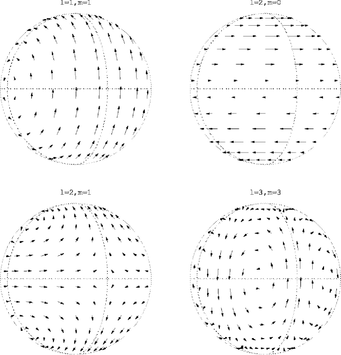
Figure 1: Velocity field on a sphere for toroidal modes (1,1), (2,0), (2,1) and (3,3) are shown at the time $t=2\pi\,n/\omega$, where $n$ is an integer, as projection on the meridional plane $\phi=-115^{\circ}$. Circles corresponding to the longitudes $0^{\circ}$ (right), -$90^{\circ}$ (left) and latitude $0^{\circ}$ are shown by dashed lines.

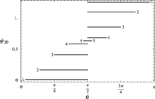
Figure 4: The potential $\Psi_{\mbox{\tiny GJ}}^{20}$ along a dipolar magnetic field line as a function of the polar angle $\theta$ is shown for 5 field lines for $t=2\pi\,n/\omega$, at which the maximal absolute values of the potential are reached. The values of $\theta$ of the left and right ends of the lines 1-5 determine the polar angle at which corresponding magnetic field line crosses the surface of the neutron star. The discontinuity is shown by the jump of $\psi$ corresponding to the same field line in the opposite hemispheres.

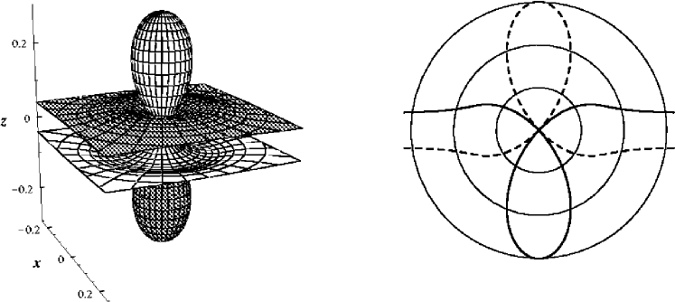
Figure 5: left: The charge density $\rho_{\mbox{\tiny GJ}}^{20}|_{r=r_{*}}$ is shown in a spherical coordinate system $(\left|\rho_{\mbox{\tiny GJ}}^{lm}|_{r=r_{*}}\right|,\theta,\phi)$ for $t=2\pi\,n/\omega$. The radial coordinate represents the absolute value of the GJ charge density as function of the polar angle $\theta$ and the azimuthal angle $\phi$. Positive values of charge density are shown by a gray surface and negative ones by white. The dipole magnetic moment ${\bf\mu}$ is directed upwards along the $z$ axis. Azimuthal angle is counted from the $x$-axis, as in Fig. 1. Note that for $\theta=\pi/2$, $\rho_{\mbox{\tiny GJ}}^{20}$ is infinite. right: Cross-section of surfaces from the left figure by a meridional plane. Circles correspond to the values 0.1, 0.2, and 0.3. Positive values are shown solid, negative ones dashed. Note that for $\theta=\pi/2$, $\rho_{\mbox{\tiny GJ}}^{20}$ is infinite.

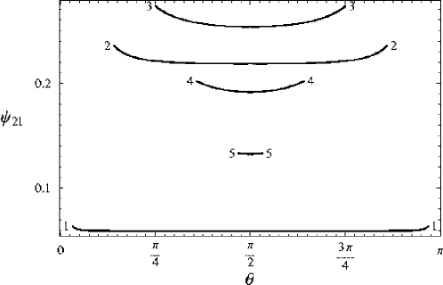
Figure 6: The potential $\Psi_{\mbox{\tiny GJ}}^{21}$ along a dipolar magnetic field line as a function of the polar angle $\theta$ is shown for 5 field lines with azimuthal angle $\phi=\pi/2$, for $t=2\pi\,n/\omega$, at which the maximal absolute values of the potential are reached. The values of $\theta$ of the left and right ends of the lines 1-5 determine the polar angle at which corresponding magnetic field line crosses the surface of the neutron star.

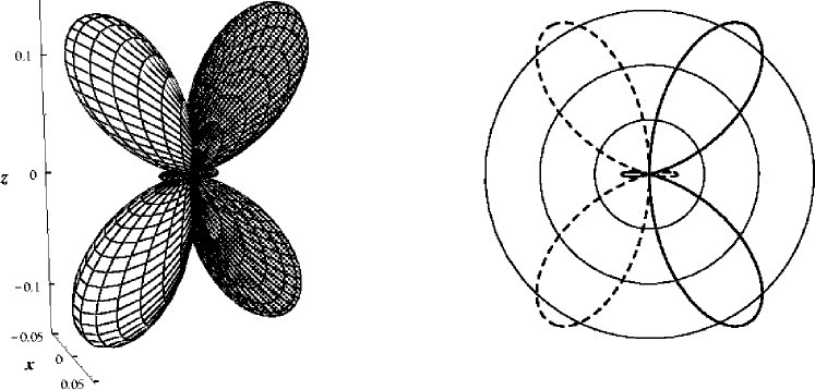
Figure 7: left: The charge density $\rho_{\mbox{\tiny GJ}}^{21}|_{r=r_{*}}$ is shown in a spherical coordinate system $(\left|\rho_{\mbox{\tiny GJ}}^{lm}|_{r=r_{*}}\right|,\theta,\phi)$ for $t=2\pi\,n/\omega$. The radial coordinate represents the absolute value of the GJ charge density as function of the polar angle $\theta$ and the azimuthal angle $\phi$. Positive values of charge density are shown by a gray surface and negative ones by white. The dipole magnetic moment ${\bf\mu}$ is directed upwards along the $z$ axis. Azimuthal angle is counted from the $x$-axis, as in Fig. 1. right: Cross-section of surfaces from the left figure by the plane $\phi=\pi/2$ , where the maximal absolute values of the charge density $\rho_{\mbox{\tiny GJ}}^{21}|_{r=r_{*}}$ are reached. Circles correspond to the values 0.05, 0.1, and 0.15. Positive values are shown solid, negative ones dashed.

In the solution for the whole region the expression (61) is used, where on the right hand side ‘$\cos\theta$‘ should be replaced by ‘$\left(1-\left(\frac{r_{*}}{r}\right)\sin^{2}\theta\right)^{1/2}$‘ for $0\leq\theta<\frac{\pi}{2}$ (first hemisphere) and by ‘$-\left(1-\left(\frac{r_{*}}{r}\right)\sin^{2}\theta\right)^{1/2}$‘ for $\frac{\pi}{2}\leq\theta\leq\pi$ (second hemisphere). Because of this there are two different expressions for $\Psi_{\mbox{\tiny GJ}}$ for both hemispheres. If these expressions give different results for $\theta=\frac{\pi}{2}$ for $r>r_{*}$ there is a discontinuity in the function $\Psi_{\mbox{\tiny GJ}}$ at the equatorial plane, and consequently $\rho_{\mbox{\tiny GJ}}(r,\frac{\pi}{2},\phi)$ becomes infinite. As we discussed in section 2.2 this unphysical result indicate that low current density approximation for such oscillation modes cannot be applied in the whole near zone. In this situation it is impossible to cancel accelerating electric field in the whole near zone without presence of a strong electric current (19) in some magnetospheric regions. Examples of such oscillation modes are modes $(l,m)=(2,0),\,(3,3)$. The corresponding velocity fields are given in Fig.1. The dependence of the potential $\Psi_{\mbox{\tiny GJ}}^{lm}$ for these modes along dipole magnetic field lines is shown in Fig.4,8. In the following we normalize the G-J potential $\Psi_{\mbox{\tiny GJ}}$ and charge density $\rho_{\mbox{\tiny GJ}}$ by $B_{0}Wr_{*}/c$ and $B_{0}W/r_{*}c$ respectively. The jump of $\Psi_{\mbox{\tiny GJ}}(r,\pi/2,\phi)$ decreases, as the angle at which corresponding magnetic field line intersect the NS‘s surface is increasing. $\Psi_{\mbox{\tiny GJ}}$ is a continuous function of $\theta$ on the surface of the NS, nevertheless GJ charge density diverges on the equator even on the surface of NS (see Fig.5, 9). In these figures the charge density $\rho_{\mbox{\tiny GJ}}^{lm}|_{r=r_{*}}$ is shown in spherical coordinates $(\left|\rho_{\mbox{\tiny GJ}}^{lm}|_{r=r_{*}}\right|,\theta,\phi)$. Here the radial coordinate represents absolute value of the GJ charge density as function of the polar angle $\theta$ and the azimuthal angle $\phi$. Analytical expressions for the GJ charge density for the discussed modes are given in Appendix C. At the equatorial plane $\rho_{\mbox{\tiny GJ}}^{lm}$ is infinite. The mode $(2,1)$ is a representative of another class of oscillation modes, in which $\Psi_{\mbox{\tiny GJ}}^{lm}$ is a continuous function of $\theta$ (see Fig.6) and $\rho_{\mbox{\tiny GJ}}^{lm}$ is finite everywhere. The velocity field and $\rho_{\mbox{\tiny GJ}}^{21}$ are shown in Figs.1, 7. For such modes it is possible to cancel longitudinal electric field without generating strong current along magnetic field lines.

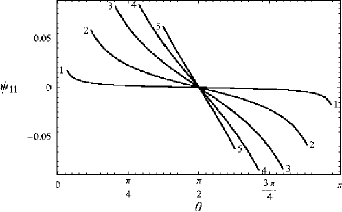
Figure 2: The potential $\Psi_{\mbox{\tiny GJ}}^{11}$ along a dipolar magnetic field line as a function of the polar angle $\theta$ is shown for 5 field lines with azimuthal angle $\phi=\pi/2$, for $t=2\pi\,n/\omega$, at which the maximal absolute values of the potential are reached. The values of $\theta$ of the left and right ends of the lines 1-5 determine the polar angle at which corresponding magnetic field line crosses the surface of the neutron star.

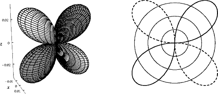
Figure 3: left: The charge density $\rho_{\mbox{\tiny GJ}}^{11}|_{r=r_{*}}$ is shown in a spherical coordinate system $(\left|\rho_{\mbox{\tiny GJ}}^{lm}|_{r=r_{*}}\right|,\theta,\phi)$ for $t=2\pi\,n/\omega$. The radial coordinate represents the absolute value of the GJ charge density as function of the polar angle $\theta$ and the azimuthal angle $\phi$. Positive values of charge density are shown by a gray surface and negative ones by white. The dipole magnetic moment ${\bf\mu}$ is directed upwards along the $z$ axis. Azimuthal angle is counted from the $x$-axis, as in Fig. 1. right: Cross-section of surfaces from the left figure by the plane $\phi=\pi/2$ , where the maximal absolute values of the charge density $\rho_{\mbox{\tiny GJ}}^{11}|_{r=r_{*}}$ are reached. Circles correspond to the values 0.01, 0.02, and 0.03. Positive values are shown solid, negative ones dashed.

Consider now the difference between two classes of toroidal oscillation modes for a NS with a dipole magnetic field. The boundary condition for $\Psi_{\mbox{\tiny GJ}}^{lm}$ is proportional to the vector product of ${\mn@boldsymbol{v}}$ and ${\mn@boldsymbol{B}}$. The axis $z$ is directed along the dipole magnetic momentum. If the velocity field is symmetric relative to the equatorial plane ($l-m$ is an odd number), then the boundary condition for $\Psi_{\mbox{\tiny GJ}}^{lm}$ is also symmetric relatively to the equatorial plane. Hence, after expression of all trigonometric functions in (61) through ‘$\cos\theta$‘ and ‘$\sin\theta$‘ , ‘$\cos\theta$‘ appears in the right hand side of (61) only in even powers. Consequently the function $\Phi^{lm}$ will be the same in both hemispheres and $\rho_{\mbox{\tiny GJ}}^{lm}$ will be finite. If velocity field is antisymmetric relative to the equatorial plane ($l-m$ is an even number or zero), then ‘$\cos\theta$‘ is contained in the right side of (61) in odd powers, and the function $\Phi^{lm}$ may have discontinuity in the plane $\theta=\frac{\pi}{2}$, and $\rho_{\mbox{\tiny GJ}}^{lm}$ for such modes becomes infinite at the equatorial plane. An example of oscillation mode with velocity field antisymmetric relative to the equatorial plane and for which $\Psi_{\mbox{\tiny GJ}}^{lm}$ is continuous function of $\theta$ is the mode $(1,1)$. Graphics for the potential $\Psi_{\mbox{\tiny GJ}}^{11}$, Goldreich-Julian charge density $\rho_{\mbox{\tiny GJ}}^{11}$ are shown in Figs. 2, 3. So, for a dipole magnetic field the longitudinal electric field generated by the oscillation modes with odd $(l-m)$ can be canceled by putting of charged particles in the magnetosphere. Among the modes with even or zero $(l-m)$ there are modes, for which longitudinal electric field cannot be canceled by putting of charged particles without presence of strong electric current along some magnetic field lines.

For an oscillation mode with odd $(l-m)$ there is a regular solution for $\rho_{\mbox{\tiny GJ}}$ and $\mn@boldsymbol{E}^{\mbox{\tiny GJ}}$ in the low current density approximation. This solution will be stable because of Lenz’s low: increasing of the current will lead to a generation of a magnetic field inducing an electric field, which will prevent the current to grow. In other words, configuration with the smallest possible current will take place. For oscillation modes with even or zero $(l-m)$, where no regular solution for GJ charge density and electric field exists, the low current density approximation cannot be used in the whole near zone. Because some of oscillation modes of this class (at least one) possess regular solution in low current density approximation, the total amount of modes, for which this approximation may be used in the whole near zone exceeds 50%.

The Goldreich-Julian charge density gives only a characteristic charge density in the magnetosphere. The particle density can be obtained by solving full system of MHD equations, but this has not been done even for an aligned rotator with a dipole magnetic field [1991]. The case of nonradial oscillation is much more complicated, because of the absence of stationarity and axial symmetry. About particle number density in the region of closed magnetic field lines we can say, that for oscillation modes with odd $(l-m)$ there can be charge separated regions in the near zone. For such modes the foot points of magnetic field lines have the same sign of the potential and there are regions where GJ charge density does not change the sign along the whole magnetic filed line. Hence, charged particles of only one sign can be pulled from the NS surface into these regions. Evidently for modes with even or zero $(l-m)$ there can not be charge-separated regions in the near zone, because GJ charge density change the sign along any magnetic field line.

3.2.2 Energy Losses

In previous works the calculation of electromagnetic energy losses of an oscillating neutron star includes only radiation of electromagnetic waves in the vacuum. If there is plasma in the magnetosphere, then the energy will be lost by a transformation of the oscillation energy into kinetic energy of an outflowing plasma, as it was proposed for pulsar energy losses by Goldreich and Julian [1969]. They obtained the energy losses of a rotating aligned NS through outflow of the charged particles from a region of open field lines, and found it to be equal to the loss in vacuum through radiation of electromagnetic waves by a perpendicular rotator. In this paper we consider electric and magnetic fields in the near zone, hence we can not explicitly show the existence of plasma outflow as in the aligned rotator by Goldreich and Julian, but a qualitatively the picture is the following. Electric current arising from the motion of the charged particles in the magnetosphere generate a magnetic field. In the region where the value of this field becomes larger than the unperturbed NS magnetic field the field lines become open, on the Alfvenic surface. Plasma escaping from the region of open field lines produces an electromagnetically driven stellar wind. The wind causes a net electric current which closes at infinity. This current flows beneath the stellar surface between positive and negative emission regions. Because it must cross magnetic field lines there, it exerts a braking torque on the oscillating NS and reduces the oscillational energy. This picture is similar to the one proposed by Ruderman & Sutherland [1975] for pulsars, but now we must get the boundary of the open field line region self-consistently. In our case we can not approximate the closed field line region by a “zone of corotation”, rather we should self-consistently determine the last closed field line as the last field line lying inside the Alfven surface.

Consider region near the pole. Let us denote as $\theta_{0}$ a polar angle by which the last closed field line intersects the surface of the NS. Similar to pulsars above a polar cap an acceleration zone and a zone of $e^{+}-e^{-}$ pair generation above it will be builded. Electron-positron pairs cancel accelerating electric field, i.e. motion of charged particle above the accelerating zone will be not influenced by electric filed generated by stellar oscillations. In the region of open field lines, where particles escape from the neutron star and form relativistic wind, the average time of crossing of the acceleration zone by the particle is much less then the oscillation period (see Discussion), so particles practically do not return back to the star. Hence, averaged over the oscillation period, the energy loss through the outflow of plasma from open field line region is

$$\epsilon^{lm}_{\rm pl}\simeq\frac{1}{\tau}\int_{0}^{\tau}\,{\rm d}t\,\int_{0}^{2\pi}\int_{0}^{\theta_{0}}\left|j^{\,lm}(r_{*},\theta,\phi)\>A^{lm}(\theta,\phi)\right|\;r_{*}^{2}\sin\theta\,{\rm d}\theta{\rm d}\phi\>,$$ (62)

where $A(\theta,\phi)$ is the work done by the electric field to move a unit charge to the point with coordinate $(r_{*},\theta,\phi)$:

$$A(\theta,\phi)\simeq\int_{0}^{\theta}E^{\mbox{\tiny GJ}}_{\theta}(r_{*},\theta^{\prime},\phi)\>r_{*}\,{\rm d}\theta^{\prime}\>.$$ (63)

Because of reasons discussed at the end of section 2.2 charge density in the inner parts of the magnetosphere must be approximately equal to the Goldreich-Julian charge density $\rho_{\mbox{\tiny GJ}}$. In the region of plasma outflow charged particles are streaming along magnetic field lines in the same direction with ultrarelativistic velocities. Charge density of outflowing plasma is equal to the Goldreich-Julian charge density. Hence, outflowing ultrarelativistic electron-positron plasma builds a net current density

$$j\simeq\rho_{\mbox{\tiny GJ}}\;c\>.$$ (64)

The current density can differ from the values given by expression (64) due to difference in averaged velocities of electron and positron components of the plasma (discussion on this topic see in Lyubarskii [1992]), but on the order of magnitude expression (64) gives good estimation for the current density [1975]. Hence, for the open field line region condition (18) is satisfied and in expression (64) we can use $\rho_{\mbox{\tiny GJ}}$ obtained by solving of equation (46) for any oscillation mode.

The last closed field line is the line for which the kinetic energy density of outflowing plasma on equator (at the point $(R_{\rm a},\pi/2,\phi)$) becomes equal to the corresponding energy density of the NS magnetic field:

$$\frac{\epsilon^{lm}_{\rm pl}(\theta_{0})}{4\pi R_{\rm a}^{2}c}\simeq\left.\frac{B^{2}}{8\pi}\right|_{\theta=\frac{\pi}{2},r=R_{\rm a}}\>.$$ (65)

Expressing the right hand side of this equation in terms of angle $\theta_{0}$, we get two equations (62), (65) for a self-consistent determination of $\theta_{0}$ and $\epsilon^{lm}_{\rm pl}$.

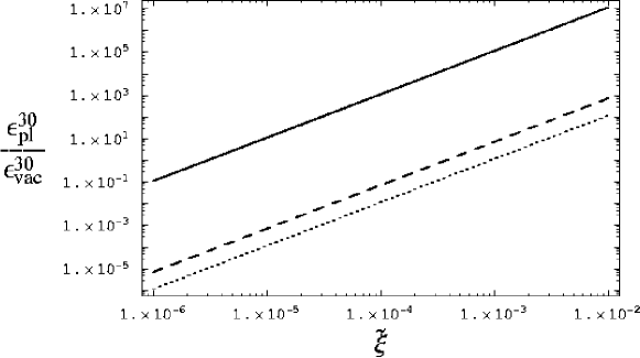
Figure 10: Ratio of the energy loss through outflow of plasma from the region of open field lines to the loss in vacuum is shown as a function of the dimensionless displacement amplitude $\tilde{\xi}$ for the mode (3,0). The solid line corresponds the oscillation period $T=19ms$ (mode ${}_{3}t_{0}$ in notations of McDermott et al. (1988)), the dashed line – $T=1.7ms$ (mode ${}_{3}t_{1}$), the dotted line – $T=1.08ms$ (mode ${}_{3}t_{2}$); see note on the page 2.

We have solved these equations for oscillation modes (1,1), (2,0), and (3,0). Oscillation periods were taken from McDermott et al. [1988]. The ratio of energy losses to the vacuum ones as a function of the amplitude of dimensionless transversal displacement $\tilde{\xi}$ for modes (1,1), (2,0), and (3,0) are given in Table 1. One can see that energy losses through outflowing plasma are much less than in vacuum for small values of $\tilde{\xi}$. On the other hand, for oscillation modes $l\geq 2$, for displacement amplitudes $\tilde{\xi}$ larger than a value $\tilde{\xi}_{\mbox{cr}}$, energy losses exceed the vacuum losses (see Fig. 10). For some oscillation modes for which $\theta_{0}\ll 1$, we can linearize equations (62), (65) in $\theta_{0}$ and get an analytical estimation of $\theta_{0}$. For toroidal oscillation mode $(l,m)$ the velocity amplitude $V$ near the pole is of the order

$$V\sim W\,\left\{\begin{array}[]{ll}\theta^{m-1},&m\neq 0\\ \theta,&m=0\end{array}\right.$$ (66)

The electric field is of the order $E^{\mbox{\tiny GJ}}\sim B\,V/c$. From formula (63) we have

$$A\sim\frac{BWr_{*}}{c}\>\left\{\begin{array}[]{ll}\theta^{m},&m\neq 0\\ \theta^{2},&m=0\end{array}\right.$$ (67)

The Goldreich-Julian charge density is

$$\rho_{\mbox{\tiny GJ}}\sim\displaystyle\frac{BW}{r_{*}c}\>\theta^{m}$$ (68)

Substituting expressions (67) and (68) into equations (64), (63) and (62) we get the energy loss through the plasma outflow along open field lines:

$$\epsilon_{\rm pl}\sim B_{0}^{2}r_{*}^{2}c\left(\frac{W}{c}\right)^{2}\>\left\{\begin{array}[]{ll}\theta_{0}^{2m+2},&m\neq 0\\ \theta_{0}^{4},&m=0\end{array}\right.$$ (69)

The angle $\theta_{0}$ is determined from the equation (65). After substitution of $\epsilon_{\rm pl}$ into equation (65) we get

$$\theta_{0}\sim\left\{\begin{array}[]{ll}\displaystyle\left(\frac{W}{c}\right)^{\frac{1}{3-m}},&m\neq 0\\ \\ \displaystyle\left(\frac{W}{c}\right)^{\frac{1}{2}},&m=0\end{array}\right.$$ (70)

We see that the angle $\theta_{0}$ is small only for modes with $m<3$. This is because of the small value of $V$ in the polar region for modes with $m\geq 3$. For such modes a linear analysis is not possible and the case of large $\theta_{0}$ needs additional investigation, which will be given elsewhere. The energy loss through plasma outflow is

$$\epsilon_{\rm pl}\sim B_{0}^{2}\,r_{*}^{2}\,c\>\left\{\begin{array}[]{ll}\displaystyle\tilde{\xi}^{\frac{8}{3-m}}\>\left(\frac{r_{*}\omega}{c}\right)^{\frac{8}{3-m}},&m=1,2\\ \\ \displaystyle\tilde{\xi}^{4}\>\left(\frac{r_{*}\omega}{c}\right)^{4},&m=0\end{array}\right.$$ (71)

The vacuum energy loss for the oscillation mode $(l,m)$, according to McDermott et al. [1984] is

$$\epsilon_{\rm vac}\sim B_{0}^{2}\,r_{*}^{2}\,c\>\tilde{\xi}^{2}\left\{\begin{array}[]{ll}\displaystyle\left(\frac{r_{*}\omega}{c}\right)^{8},&l=1,m=0\\ \\ \displaystyle\left(\frac{r_{*}\omega}{c}\right)^{2l+2},&l=1,m=1;\,l\geq 2,m=0\dots l\\ \end{array}\right.$$ (72)

From these formulas we get the oscillation amplitude $\tilde{\xi}$ for which the plasma energy loss is larger than the vacuum loss

$$\tilde{\xi}>\tilde{\xi}_{\mbox{cr}}\sim\left\{\begin{array}[]{ll}\displaystyle\left(\frac{r_{*}\omega}{c}\right)^{2},&l=1,m=0\\ \\ \displaystyle\left(\frac{r_{*}\omega}{c}\right)^{l-1},&l\geq 2,m=0;\,l\geq 1,m=1\\ \\ \displaystyle\left(\frac{r_{*}\omega}{c}\right)^{l/3-1},&l\geq 2,m=2\end{array}\right.$$ (73)

From formula (73) it follows that for modes $(l=1,m=0)$, $(l\geq 2,m=0,1)$ and $(l\geq 4,m=2)$ nonvacuum energy loss exceeds the vacuum loss even for small displacement amplitudes $\tilde{\xi}$, because for these modes $\tilde{\xi}_{\mbox{cr}}\ll 1$.

Mode $\epsilon_{\rm pl}/\epsilon_{\rm vac}$ $R^{lm}_{\rm a}/\lambda$ $(1,1)$ $0.02\>\tilde{\xi}^{2}$ $0.9/\tilde{\xi}$ $(2,0)$ $77\>\tilde{\xi}^{2}\tau^{2}$ $0.2/\tilde{\xi}$ $(3,0)$ $9\cdot 10^{5}\>\tilde{\xi}^{2}\tau^{4}$ $0.09/\tilde{\xi}$

Table 1: Leading terms in expansion over $\tilde{\xi}$ of ratios of electromagnetic energy loss through plasma outflow to the vacuum one $\epsilon_{\rm pl}/\epsilon_{\rm vac}$ and distance in the equatorial plane of the last closed field line to the wave length $R^{lm}_{\rm a}/\lambda$ for toroidal oscillation modes $(1,1)$, $(2,0)$ and $(3,0)$. $\tau$ is period of oscillations in milliseconds.

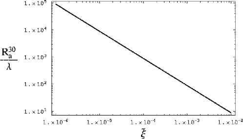
Figure 11: Ratio of the equatorial radius of the last closed field line to the wavelength $\lambda$ is shown as a function of the dimensionless displacement amplitude $\tilde{\xi}$ for the mode (3,0). This ratio does not depend on the oscillation frequency $\omega$.

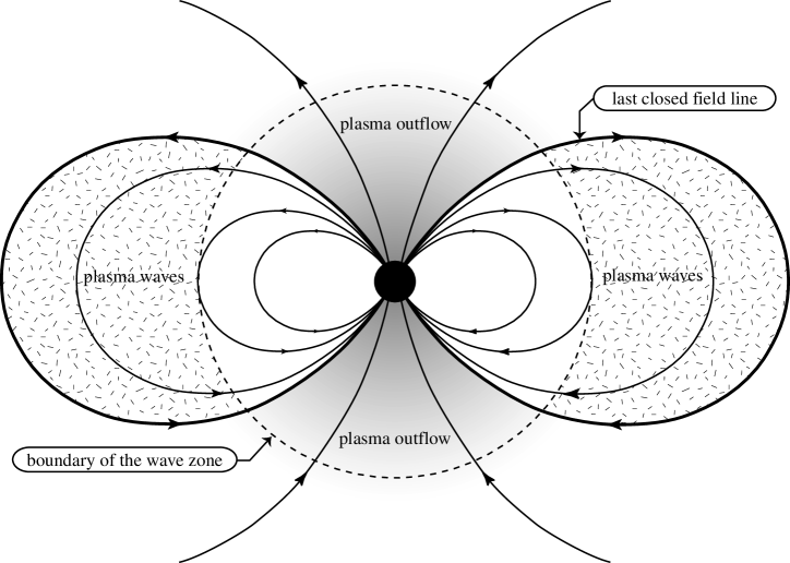
Figure 12: Structure of the magnetosphere of an oscillating neutron star (arbitrary scaled). See explanations in text.

Electromagnetic waves radiated by the oscillating NS are screened by the plasma. For small $\tilde{\xi}$ the nonvacuum energy loss according to (73) is smaller than the vacuum loss because at the GJ density of particles the accelerated plasma cannot escape from the magnetosphere. The ratio of the equatorial radius for the last closed field line, to the wave length $\lambda$ are given in Table 1. For mode $(3,0)$ this dependence is shown in Fig. 11. We see that the last closed field line for small values of displacement amplitude lies deep inside the wave zone. In the region limited by the last closed field lines and a sphere of radius $\lambda$ (formal boundary of the wave zone) in this situation confined plasma waves are excited such as Alfven or magnetosonic wave by the oscillation of the NS, see Fig. 12. This will lead to accumulation of energy in this region in the form of plasma wave energy. When the density of this energy becomes larger than the magnetic energy, field lines becomes open. These processes will lead to a decrease of the equatorial radius of the last closed field lines, and hence, a increase of the energy loss.

A second process which could lead to larger energy losses than obtained by the solution of the equation (65), is rotation of the neutron star. In this case the equatorial radius of the last closed field line is the radius of the light cylinder $R_{\small L}=\Omega/c$, and surface area for plasma outflow may be considerably increased. It is not clear, however, how the interaction between rotation an oscillation will influence the total energy losses.

4 Discussion

Under the assumption of low current density we have developed a formalism describing the inner parts of the magnetosphere of an oscillating neutron star in the same way as in the case of rotation. This assumption is valid in the region of open field lines for any oscillation mode. For some oscillation modes the assumption about low current density everywhere in the inner magnetosphere leads to unphysical results – the Goldreich-Julian charge density becomes infinite in some points. For such oscillation modes the low current density approximation cannot be used in the whole region of closed magnetic field lines near the NS. The current density for these modes along some closed magnetic field lines will be of the order of magnitude $j\simeq\frac{c}{\omega r}\,\rho_{\mbox{\tiny GJ}}\>c$. For a rotating neutron star our formalism yields the same values for the Goldreich-Julian charge density and electric field as obtained in works of Goldreich and Julian [1969] and Mestel [1971].

We applied the general formalism to the case of toroidal oscillations of a neutron star with dipole magnetic field. We calculated the GJ charge density and showed, that for the case considered the assumption about low current density in the whole inner magnetosphere is valid for more than half of all modes. We calculated the electromagnetic energy losses of a NS with dipole magnetic field for some toroidal oscillation modes and showed, that the energy losses of an oscillating neutron star are strongly affected by the plasma present in its magnetosphere. Electromagnetic energy losses of an oscillating NS due to plasma outflow from the magnetosphere have in general another dependence on oscillation frequency $\omega$ and the dimensionless displacement amplitude $\tilde{\xi}$ than the energy losses due to radiation of electromagnetic waves in vacuum. This affects all previous calculations of the electromagnetic damping rate of NS oscillation. Our calculations give a lower limit on electromagnetic energy losses of an oscillating NS because of the reasons discussed at the end of section 3.2.2. The energy of a star oscillation depends on the dimensionless displacement amplitude as $\tilde{\xi}^{2}$. Energy losses through plasma outflow in contrast to energy losses through radiation of electromagnetic waves in vacuum have another dependence on the displacement amplitude. Consequently the electromagnetic energy losses of an oscillating NS in general depends on the oscillation amplitude $\tilde{\xi}$. To estimate the oscillation damping time for the considered oscillation modes one can use values given in McDermott et al. [1988], Table 6, multiplying by functions from Table 1 of this paper for a given displacement amplitude. Here we have restricted ourselves to a simple case of toroidal oscillations. Starquakes should excite a whole spectrum of oscillations, including $p$- and $g$- modes. The magnetosphere structure produced by these modes will be considered in a future paper.

With the proposed formalism it is possible to apply theoretical models developed for pulsars to oscillating neutron stars. For example, one can investigate the acceleration mechanism proposed by Scharlemann, Arons & Fawley [1978] or by Ruderman & Sutherland [1975] for oscillating neutron star. The inertial frame dragging mechanism proposed by Muslimov & Tsygan [1992] does not work here, because we consider a nonrotating star. Characteristic time of pair cascade formation is estimated as $h_{\rm PPF}/c$, where $h_{\rm PPF}$ is the hight of pair formation front above the surface. In “Ruderman-Sutherland” model minimum value of $h_{\rm PPF}$ is the same as for a NS rotating with the angular frequency $\Omega_{\rm eff}=\omega\tilde{\xi}$, and for usually assumed parameters of NS oscillation is of order $10^{4}-10^{5}$ cm. In “Arons-Scharlemann” like model the hight of pair formation front can be smaller then in a pulsar rotating with the angular frequency $\Omega_{\rm eff}$ (several km), because in general for nonradial oscillation ratio $\rho_{\mbox{\tiny GJ}}/B$ along magnetic field lines increase faster than in magnetosphere of a rotating NS, what leads to larger accelerating electric fields. Because the characteristic time of pair cascade formation is much shorter than the period of oscillation, one can consider the polar cap acceleration zone in any given moment of time as stationary. Problem of return current region for the case of oscillating NS as in the case of pulsar remains open. Similar to pulsars return current can flow along the last closed magnetic field line.

The authors wish to thank A. I. Tsygan for helpful discussions. This work has been supported by Russian Foundation of Basic Research (RFFI) under grants 96-02-16553 and 99-02-18180.

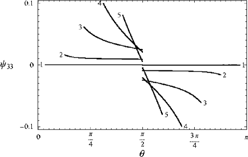
Figure 8: The potential $\Psi_{\mbox{\tiny GJ}}^{33}$ along a dipolar magnetic field line as a function of the polar angle $\theta$ is shown for 5 field lines with azimuthal angle $\phi=\pi/6$, for $t=2\pi\,n/\omega$, at which the maximal absolute values of the potential are reached. The values of $\theta$ of the left and right ends of the lines 1-5 determine the polar angle at which corresponding magnetic field line crosses the surface of the neutron star. The discontinuity is shown by the jump of $\psi$ corresponding to the same field line in the opposite hemispheres.

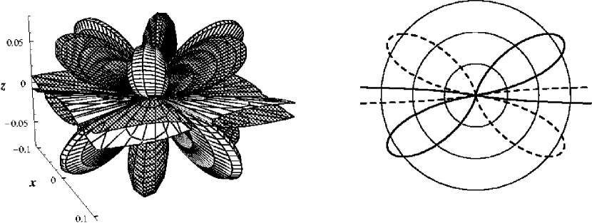
Figure 9: left: The charge density $\rho_{\mbox{\tiny GJ}}^{33}|_{r=r_{*}}$ is shown in a spherical coordinate system $(\left|\rho_{\mbox{\tiny GJ}}^{lm}|_{r=r_{*}}\right|,\theta,\phi)$ for $t=2\pi\,n/\omega$. The radial coordinate represents the absolute value of the GJ charge density as function of the polar angle $\theta$ and the azimuthal angle $\phi$. Positive values of charge density are shown by a gray surface and negative ones by white. The dipole magnetic moment ${\bf\mu}$ is directed upwards along the $z$ axis. Azimuthal angle is counted from the $x$-axis, as in Fig. 1. Note that for $\theta=\pi/2$, $\rho_{\mbox{\tiny GJ}}^{33}$ is infinite. right: Cross-section of surfaces from the left figure by the plane $\phi=\pi/6$ , where the maximal absolute values of the charge density $\rho_{\mbox{\tiny GJ}}^{33}|_{r=r_{*}}$ are reached. Circles correspond to the values 0.04, 0.08, and 0.12. Positive values are shown solid, negative ones dashed. Note that for $\theta=\pi/2$, $\rho_{\mbox{\tiny GJ}}^{33}$ is infinite.

APPENDIX

Appendix A Calculation of $P$ and $\delta P$

Substituting ${\mn@boldsymbol{B}}$ from formula (26) using expansion (34) into the equation (20) we have

$${\mn@boldsymbol{\nabla}}{\mn@boldsymbol{\times}}{\mn@boldsymbol{\nabla}}{\mn@boldsymbol{\times}}{\mn@boldsymbol{\nabla}}{\mn@boldsymbol{\times}}(P_{0}+\delta P){\mn@boldsymbol{e}_{r}}=0\>.$$ (74)

Because $P$ does not depend on $t$, equation (74) is equivalent to the following two equations:

$${\mn@boldsymbol{\nabla}}{\mn@boldsymbol{\times}}{\mn@boldsymbol{\nabla}}{\mn@boldsymbol{\times}}{\mn@boldsymbol{\nabla}}{\mn@boldsymbol{\times}}(P_{0}{\mn@boldsymbol{e}_{r}})=0\>\phantom{.}$$ (75)

$${\mn@boldsymbol{\nabla}}{\mn@boldsymbol{\times}}{\mn@boldsymbol{\nabla}}{\mn@boldsymbol{\times}}{\mn@boldsymbol{\nabla}}{\mn@boldsymbol{\times}}(\delta P{\mn@boldsymbol{e}_{r}})=0\>.$$ (76)

In spherical coordinate equation (76) is

$${\mn@boldsymbol{\nabla}}{\mn@boldsymbol{\times}}{\mn@boldsymbol{\nabla}}{\mn@boldsymbol{\times}}{\mn@boldsymbol{\nabla}}{\mn@boldsymbol{\times}}(\delta P{\mn@boldsymbol{e}_{r}})=-{\bf e}_{\theta}\frac{1}{r\sin\theta}\left(\frac{1}{r^{2}}\>\partial_{\phi}\,\Delta_{\Omega}\delta P+\partial_{rr}\partial_{\phi}\delta P\right)+{\bf e}_{\phi}\frac{1}{r}\left(\frac{1}{r^{2}}\>\partial_{\theta}\,\Delta_{\Omega}\delta P+\partial_{rr}\partial_{\theta}\delta P\right)=0\>.$$ (77)

Substituting expansion of $\delta P$ (35) we get

$$-\frac{1}{r^{2}}l(l+1)\delta\tilde{p}_{lm}(r,t)+\partial_{rr}\delta\tilde{p}_{lm}(r,t)=0\>.$$ (78)

The solution of equation (78) which vanishes at infinity is

$$\delta\tilde{p}_{lm}(r,t)=\left(\frac{r_{*}}{r}\right)^{l}\delta p_{lm}(t)\>.$$ (79)

The time-dependent coefficients $p_{lm}(t)$ have to be determined from the boundary conditions. Substituting expression (A6) into expansion (35) and taking the derivative with respect to $t$ we get expression (36).

Similarly, for the coefficients $P_{0\,lm}$ in the expansion of the function $P_{0}$ we have

$$P_{0\,lm}(r)=p_{lm}\left(\frac{r_{*}}{r}\right)^{l}$$ (80)

Substituting the expansion of the function $P_{0}$ in spherical harmonics into the boundary condition (11), multiplying this expression by $Y^{*}_{lm}$, and integrating it over solid angle $4\pi$, we have (compare with formula (16) in Muslimov & Tsygan [1986])

$$p_{lm}=\frac{r_{*}^{2}}{l(l+1)}\int_{4\pi}B_{0\,r}Y^{*}_{lm}\,{\rm d}\Omega,$$ (81)

where $Y^{*}_{lm}$ is inverse spherical harmonic $\int Y_{lm}Y^{*}_{l^{\prime}m^{\prime}}\,{\rm d}\Omega=\delta_{ll^{\prime}}\delta_{mm^{\prime}}$ and ${\rm d}\Omega=\sin\theta{\rm d}\theta\,{\rm d}\phi$ is the solid angle

Appendix B Calculation of $\delta p_{lm}(t)$

Differentiating equation (41) with respect to $\phi$ and equation (42) with respect to $\theta$, equating the results and multiplying by $1/\sin\theta$ we have

$$\left.\left[\frac{1}{\sin\theta}\partial_{\theta}(\sin\theta\,\partial_{\theta}(\partial_{t}P))+\frac{1}{\sin^{2}\theta}\partial_{\phi\phi}(\partial_{t}P)\right]\right|_{r=r_{*}} = -\left\{\,\frac{1}{r}\Delta_{\Omega}P\left[\frac{1}{\sin\theta}\partial_{\theta}(\sin\theta\>v_{\theta})+\frac{1}{\sin\theta}\partial_{\phi}\ v_{\phi}\right]\right.+$$ (82)

$$\phantom{-\{.}\left.\left.\left[\frac{1}{\sin\theta}\partial_{\theta}(\sin\theta\>\partial_{r}\partial_{\theta}P)+\frac{1}{\sin^{2}\theta}\partial_{r}\partial_{\phi\phi}P\right]\;v_{r}+\right.\right.$$

$$\phantom{-\{.}\left.\left.\left[\frac{1}{r}\partial_{\theta}\Delta_{\Omega}P\;v_{\theta}+\frac{1}{r\sin\theta}\partial_{\phi}\Delta_{\Omega}P\;v_{\phi}\right]+\right.\right.$$

$$\phantom{-\{.}\left.\left.\left[\partial_{r}\partial_{\theta}P\;\partial_{\theta}v_{r}+\frac{1}{\sin^{2}\theta}\partial_{r}\partial_{\phi}P\;\partial_{\phi}v_{r}\right]\,\right\}\right|_{r=r_{*}}$$

Simplifying equation (82) by writing $P$ as a sum of the two terms (34), we get an expression for time-dependent part $\delta P$ to first order in $\tilde{\xi}$

$$\left.\partial_{t}\Delta_{\Omega}\delta P\right|_{r=r_{*}} = -\left[\,\left(v_{r}\;\partial_{r}\Delta_{\Omega}P_{0}+v_{\theta}\;\frac{1}{r}\partial_{\theta}\Delta_{\Omega}P_{0}+v_{\phi}\;\frac{1}{r\sin\theta}\partial_{\phi}\Delta_{\Omega}P_{0}\right)+\Delta_{\Omega}P_{0}\left(\frac{1}{r\sin\theta}\partial_{\theta}(\sin\theta\>v_{\theta})+\frac{1}{r\sin\theta}\partial_{\phi}\ v_{\phi}\right)\right.+$$ (83)

$$\phantom{-[.}\left.\left.\left(\partial_{r}\partial_{\theta}P_{0}\;\partial_{\theta}v_{r}+\frac{1}{\sin^{2}\theta}\partial_{r}\partial_{\phi}P_{0}\;\partial_{\phi}v_{r}\right)\,\right]\right|_{r=r_{*}}$$

or in vector notation

$$\left.\partial_{t}\Delta_{\Omega}\delta P\right|_{r=r_{*}}=-\left.\left\{{\mn@boldsymbol{v}}\cdot{\mn@boldsymbol{\nabla}}(\Delta_{\Omega}P_{0})+\Delta_{\Omega}P_{0}({\mn@boldsymbol{\nabla}}\cdot{\mn@boldsymbol{v}}_{\perp})+r^{2}({\mn@boldsymbol{\nabla}}_{\perp}(\partial_{r}P_{0})\cdot{\mn@boldsymbol{\nabla}}_{\perp})\,v_{r}\right\}\right|_{r=r_{*}},$$ (84)

where ${\mn@boldsymbol{v}}_{\perp}$ is the tangential part of the velocity, ${\mn@boldsymbol{v}}_{\perp}={\bf e}_{\theta}\>v_{\theta}+{\bf e}_{\phi}\>v_{\phi}$, and ${\mn@boldsymbol{\nabla}}_{\perp}$ is the angular part of the gradient: ${\mn@boldsymbol{\nabla}}_{\perp}={\bf e}_{\theta}\>1/r\>\partial_{\theta}+{\bf e}_{\phi}\>1/(r\sin\theta)\>\partial_{\phi}$. Substituting the expansion of $\delta P$ in spherical harmonics (36), multiplying the result by $Y^{*}_{lm}$ and integrating it over the solid angle $4\pi$, we get an expression for the coefficients of $\partial_{t}\delta p(t)$ (43) in the expansion of $\delta P$ in spherical harmonics:

$$\partial_{t}\delta p_{lm}(t)=\frac{1}{l(l+1)}\int_{4\pi}\,{\rm d}\Omega\;Y^{*}_{lm}\left.\left[{\mn@boldsymbol{v}}\cdot{\mn@boldsymbol{\nabla}}(\Delta_{\Omega}P_{0})+\Delta_{\Omega}P_{0}({\mn@boldsymbol{\nabla}}\cdot{\mn@boldsymbol{v}}_{\perp})+r^{2}({\mn@boldsymbol{\nabla}}_{\perp}(\partial_{r}P_{0})\cdot{\mn@boldsymbol{\nabla}}_{\perp})\,v_{r}\right]\right|_{r=r_{*}}\>.$$

Next we give explicit expressions for coefficients $\delta p_{lm}(t)$ for toroidal and spheroidal oscillations modes (see Unno et al. [1979]). Spheroidal separation of variables gives the following expressions for components of the oscillation velocity in spherical coordinates

$$v_{r}=e^{-{\rm i}\omega t}\>U(r)\>Y_{lm}(\theta,\phi),\quad v_{\theta}=e^{-{\rm i}\omega t}\>V(r)\>\partial_{\theta}Y_{lm}(\theta,\phi),\quad v_{\phi}=e^{-{\rm i}\omega t}\>V(r)\>\frac{1}{\sin\theta}\partial_{\phi}Y_{lm}(\theta,\phi)\>,$$ (85)

where $U$ and $V$ are radial and transversal velocity amplitude respectively. Substituting the velocity components (85) into formula (36), we get the coefficients $\partial_{t}\delta p_{l^{\prime}m^{\prime}}(t)$ for spheroidal oscillations

$$\partial_{t}\delta p_{l^{\prime}m^{\prime}}(t) = \frac{e^{-{\rm i}\omega t}}{l^{\prime}(l^{\prime}+1)}\int_{4\pi}\,{\rm d}\Omega\;Y^{*}_{l^{\prime}m^{\prime}}\;\left[\,U\left(Y_{lm}\;\partial_{r}\Delta_{\Omega}P_{0}+\partial_{\theta}Y_{lm}\;\partial_{\theta}\partial_{r}P_{0}+\frac{1}{\sin^{2}\theta}\partial_{\phi}Y_{lm}\;\partial_{\phi}\partial_{r}P_{0}\right)+\right.$$ (86)

$$\phantom{\frac{1}{l^{\prime}(l^{\prime}+1)}\int_{4\pi}\,{\rm d}\Omega\;Y^{*}_{l^{\prime}m^{\prime}}[.}\left.\left.\frac{V}{r}\left(-l(l+1)\;Y_{lm}\;\Delta_{\Omega}P_{0}+\partial_{\theta}Y_{lm}\;\partial_{\theta}\Delta_{\Omega}P_{0}+\frac{1}{\sin^{2}\theta}\partial_{\phi}Y_{lm}\;\partial_{\phi}\Delta_{\Omega}P_{0}\right)\,\right]\right|_{r=r_{*}}$$

The oscillation velocity components for toroidal oscillations are

$$v_{r}=0,\quad v_{\theta}=e^{-{\rm i}\omega t}\>W(r)\>\frac{1}{\sin\theta}\partial_{\phi}Y_{lm}(\theta,\phi),\quad v_{\phi}=-e^{-{\rm i}\omega t}\>W(r)\>\partial_{\theta}Y_{lm}(\theta,\phi)\>,$$ (87)

where $W$ is transversal velocity amplitude. With the use of formula (87), the coefficients in the expansion of $\partial_{t}\delta P$ for toroidal oscillations are

$$\partial_{t}\delta p_{l^{\prime}m^{\prime}}(t)=\frac{e^{-{\rm i}\omega t}}{l^{\prime}(l^{\prime}+1)}\int_{4\pi}\,{\rm d}\Omega\;Y^{*}_{l^{\prime}m^{\prime}}\;\left.\left[W\frac{1}{r\sin\theta}\left(\partial_{\phi}Y_{lm}\;\partial_{\theta}\Delta_{\Omega}P_{0}-\partial_{\theta}Y_{lm}\;\partial_{\phi}\Delta_{\Omega}P_{0}\right)\right]\right|_{r=r_{*}}\>.$$ (88)

Appendix C Expressions for Goldreich-Julian charge density
for modes (1,1), (2,0), (2,1), (3,3)

$\rho_{\mbox{\tiny GJ}}^{11}$ for $0\leq\theta\leq\pi$

$$\rho_{\mbox{\tiny GJ}}^{11}=e^{-i\omega t}\frac{3\,{\sqrt{\frac{3}{2}}}\,B\,W\,\cos(\theta)\,\sin(\theta)\,\sin(\phi)\,{r_{*}}^{2}}{8\,c\,{\pi}^{\frac{3}{2}}\,r^{3}}$$ (89)

$\rho_{\mbox{\tiny GJ}}^{20}$ for $0\leq\theta<\frac{\pi}{2}$

$$\rho_{\mbox{\tiny GJ}}^{20}=-e^{-i\omega t}\frac{3\,{\sqrt{5}}\,B\,W\,{{r_{*}}}^{2}\,\left(16\,r-3\,{r_{*}}+15\,\cos(4\,\theta)\,{r_{*}}-12\,\cos(2\,\theta)\,\left(-4\,{r}+{{{r}}_{*}}\right)\right)}{256\,c\,{\pi}^{\frac{3}{2}}\,r^{4}\,{\sqrt{1-\frac{{\sin(\theta)}^{2}\,{r_{*}}}{r}}}}$$ (90)

$\rho_{\mbox{\tiny GJ}}^{20}$ for $\frac{\pi}{2}<\theta\leq\pi$

$$\rho_{\mbox{\tiny GJ}}^{20}=e^{-i\omega t}\frac{3\,{\sqrt{5}}\,B\,W\,{{r_{*}}}^{2}\,\left(16\,r-3\,{r_{*}}+15\,\cos(4\,\theta)\,{r_{*}}-12\,\cos(2\,\theta)\,\left(-4\,{r}+{r_{*}}\right)\right)}{256\,c\,{\pi}^{\frac{3}{2}}\,r^{4}\,{\sqrt{1-\frac{{\sin(\theta)}^{2}\,{r_{*}}}{r}}}}$$ (91)

$\rho_{\mbox{\tiny GJ}}^{21}$ for $0\leq\theta\leq\pi$

$$\rho_{\mbox{\tiny GJ}}^{21}=e^{-i\omega t}\frac{{\sqrt{\frac{5}{6}}}\,B\,W\,\sin(\theta)\,\sin(\phi)\,{r_{*}}^{\frac{3}{2}}\,\left(21\,r+19\,{r_{*}}+45\,\cos(2\,\theta)\,{r_{*}}\right)}{32\,c\,{\pi}^{\frac{3}{2}}\,r^{\frac{7}{2}}}$$ (92)

$\rho_{\mbox{\tiny GJ}}^{33}$ for $0\leq\theta<\frac{\pi}{2}$

$$\rho_{\mbox{\tiny GJ}}^{33} = e^{-i\omega t}\frac{3\,{\sqrt{35}}\,B\,W\,{\sin(\theta)}^{3}\,\sin(3\,\phi)\,{r_{*}}^{\frac{5}{2}}}{256\,c\,{\pi}^{\frac{3}{2}}\,r^{\frac{11}{2}}\,{\sqrt{1-\frac{{\sin(\theta)}^{2}\,{r_{*}}}{r}}}}\,\left(\vphantom{\sqrt{\cos(2\theta)}}15\,r^{2}+2\,r\,{r_{*}}+6\,\cos(4\,\theta)\,{r_{*}}^{2}-\right.$$ (94)

$$\qquad\qquad\left.6\,\cos(2\,\theta)\,{r_{*}}\,\left(-5\,r+{r_{*}}\right)-6\,{\sqrt{2}}\,\cos(3\,\theta)\,{r_{*}}^{\frac{3}{2}}\,{\sqrt{2\,r-{r_{*}}+\cos(2\,\theta)\,{r_{*}}}}\ \right)$$

$\rho_{\mbox{\tiny GJ}}^{33}$ for $\frac{\pi}{2}<\theta\leq\pi$

$$\rho_{\mbox{\tiny GJ}}^{33} = -e^{-i\omega t}\frac{3\,{\sqrt{35}}\,B\,W\,{\sin(\theta)}^{3}\,\sin(3\,\phi)\,{r_{*}}^{\frac{5}{2}}}{256\,c\,{\pi}^{\frac{3}{2}}\,r^{\frac{11}{2}}\,{\sqrt{1-\frac{{\sin(\theta)}^{2}\,{r_{*}}}{r}}}}\,\left(15\,r^{2}+2\,r\,{r_{*}}+6\,\cos(4\,\theta)\,{r_{*}}^{2}-\right.$$ (96)

$$\qquad\qquad\left.6\,\cos(2\,\theta)\,{r_{*}}\,\left(-5\,r+{r_{*}}\right)+6\,{\sqrt{2}}\,\cos(3\,\theta)\,{r_{*}}^{\frac{3}{2}}\,{\sqrt{2\,r-{r_{*}}+\cos(2\,\theta)\,{r_{*}}}}\ \right)$$

References

- [1995] Bisnovatyi-Kogan G. S., 1995, ApJS 97, 185
- [1975] Bisnovatyi-Kogan G. S., Imshennik V. S., Nadiozhin D. K., Chechetkin V. M., 1975, Ap&SS, 35, 23
- [1989] Blaes O., Blandford R., Goldreich P., Madau P., 1989, ApJ, 343, 839
- [1976] Boriakoff V., 1976, ApJ, 208, L43
- [1947] Brandt L., 1947, Vector and Tensor Analysis. John Wiley & Sons, Inc., New York
- [1986] Carroll B. W., Zweibel E. G., Hansen C. J., McDermott P. N., Savedoff M. P., Thomas J. N., Van Horn H. M., 1986, ApJ, 305, 767
- [1982] Daugherty J. K., Harding A. K., 1982, ApJ, 252, 337
- [1997] Ding K. Y., Cheng K. S., 1997, MNRAS, 287, 671
- [1998] Duncan R. C., 1998, ApJ, 498, L45
- [1965] Elsgolts L. E., 1965, Differentsialnye uravneniya i variatsionnoe ischislenie. Nauka, Moskva (in Russian)
- [1993] Fatuzzo M., Melia F., 1993, ApJ, 407, 680
- [1969] Goldreich P., Julian W. H., 1969, ApJ, 157, 869
- [1996] Hankins T. H., 1996, in Astronomical Society of the Pacific Conference Series, Vol. 105, IAU Colloquium 160, Pulsars: Problems and Progress ed. S. Johnston, M. A. Walker & M. Bailes, 197
- [1994] Hurley K., et al., 1994, Nat, 372, 652
- [1986] Jones P. B., 1986, MNRAS, 218, 477
- [1996] Lyne A. G., 1996, in Astronomical Society of the Pacific Conference Series, Vol. 105, IAU Colloquium 160, Pulsars: Problems and Progress ed. S. Johnston, M. A. Walker & M. Bailes, 73
- [1992] Lyubarskii Yu. E., 1992, A&A, 261, 544
- [1988] McDermott P. N., Van Horn H. M., Hansen C. J., 1988, ApJ, 325, 725
- [1984] McDermott P. N., Savedoff M. P., Van Horn H. M., Zweibel E. G., Hansen C. J., 1984, ApJ, 281, 746
- [1971] Mestel L., 1971, Nature Physical Science, 233, 149
- [1991] Michel F. C., 1991, Theory of neutron star magnetospheres. University of Chicago Press, Chicago
- [1986] Muslimov A. G., Tsygan A. I., 1986, Ap&SS, 120, 27
- [1992] Muslimov A. G., Tsygan A. I., 1992, MNRAS, 255, 61
- [1974] Pacini F., Ruderman M., 1974, Nat, 251, 399
- [1975] Ruderman M. A., Sutherland P. G., 1975, ApJ, 196, 51
- [1978] Scharlemann E. T., Arons J., Fawley W. M., 1978, ApJ, 222, 297
- [1993] Smith I. A., Epstein R. I., 1993, ApJ, 410, 315
- [1991] Strohmayer T. E., 1991, ApJ, 372, 573
- [1971] Sturrock P. A., 1971, ApJ, 164, 529
- [1998] Trümper J., Becker W., 1998, Advances in Space Research, 21, 203
- [1975] Tsygan A. I., 1975, A&A, 44, 21
- [1979] Unno W., Osaki Y., Ando H., Shibahashi H., 1979, Nonradial Oscillations of Stars. University of Tokyo Press, Tokyo
- [1996] Wolfram S., 1996, The Mathematica book, Third Edition. Wolfram Media/Cambridge University Press, Champaign, Illinois