Limits on Stellar and Planetary Companions in Microlensing Event OGLE-1998-BUL-14

Abstract

We present the PLANET photometric data set for OGLE-1998-BUL-14, a high magnification ($A_{\rm max}\sim 16$) event alerted by the OGLE collaboration toward the Galactic bulge in 1998. The PLANET data set consists a total of $461$ $I-$band and $139$ $V-$band points, the majority of which was taken over a three month period. The median sampling interval during this period is about 1 hour, and the $1\sigma$ scatter over the peak of the event is $1.5\%$. The excellent data quality and high maximum magnification of this event make it a prime candidate to search for the short duration, low amplitude perturbations that are signatures of a planetary companion orbiting the primary lens. The observed light curve for OGLE-1998-BUL-14 is consistent with a single lens (no companion) within photometric uncertainties. We calculate the detection efficiency of the light curve to lensing companions as a function of the mass ratio and angular separation of the two components. We find that companions of mass ratio $\geq 0.01$ are ruled out at the 95% confidence level for projected separations between $0.4-2.4{r_{\rm E}}$, where ${r_{\rm E}}$ is the Einstein ring radius of the primary lens. Assuming that the primary is a G-dwarf with ${r_{\rm E}}\sim 3~{}{\rm AU}$ our detection efficiency for this event is $\sim 60\%$ for a companion with the mass and separation of Jupiter and $\sim 5\%$ for a companion with the mass and separation of Saturn. Our efficiencies for planets like those around Upsilon And and 14 Her are $>75\%$.

1. Introduction

Mao & Paczyński (1991) first suggested that planets could be detected in microlensing events; Gould & Loeb (1992) pointed out that if all stars had Jupiter-mass planets with separations near $5~{}{\rm AU}$, then $\sim 20\%$ of the microlensing events should exhibit detectable planetary deviations, provided that events were monitored frequently and with moderately high precision. Current microlensing discovery teams do not generally sample frequently or precisely enough to detect the short-lived perturbations caused by planets. However, since these collaborations reduce their data in real time, they are able to issue ‘alerts,’ notification of ongoing microlensing events detected before the peak magnification. Prompted by this alert capability, several other groups have formed to monitor alerted microlensing events more closely (GMAN, Alcock et al. 1997; PLANET, Albrow et al. 1998; MPS, Rhie et al. 1999a). Since only a handful of alerted events are in progress at any given time, they can be monitored with the fine temporal sampling and photometric precision required to discover planetary perturbations. In particular, the PLANET (Probing Lensing Anomalies NETwork) collaboration has access to four telescopes that are roughly equally-spaced in longitude, and thus can monitor microlensing events almost continuously, weather permitting.

Over the last five years, PLANET has monitored over 100 events with varying degrees of sampling and photometric precision. Here we present photometry and analysis of one such event, OGLE-1998-BUL-14, the 14th event alerted by the OGLE collaboration toward the Galactic bulge in 1998. The total PLANET data set for this event consists of 600 data points, the majority of which was taken during a 3 month period starting 1 May 1998. The median sampling interval during this interval is about $1~{}{\rm hour}$, with no gaps greater than 4 days. The photometric precision near the peak of the event, where the sensitivity to planets is highest, is $1.5\%$. These characteristics, combined with the high maximum magnification of OGLE-1998-BUL-14 make our data set highly sensitive to planetary perturbations. The PLANET data for the event are consistent with a generic point-source point-lens (PSPL) model. The excellent photometry and dense sampling also allow us to place stringent constraints on possible stellar and planetary companions. We also place limits on parallax effects arising from the motion of the Earth, deviations arising from the finite size of the source, and the amount of blended light from the lens itself. These limits are then translated into limits on the mass of the lens. We find that, despite the excellent coverage and photometry of OGLE-1998-BUL-14, the limits on the mass of the lens are very weak. This indicates that it will in general be quite difficult to obtain interesting constraints on the masses of the lenses giving rise to microlensing events from photometric data alone.

Our study is similar to that done by the MPS and MOA collaborations on the microlensing event MACHO-1998-BLG-35 (Rhie et al. 1999b ), which was a higher maximum magnification event ($A_{\rm max}\sim 75$) than OGLE-1998-BUL-14. We compare the limits on companions for OGLE-1998-BUL-14 to those for MACHO-1998-BLG-35 directly in § 5.2.

A brief introduction to the theory of microlensing is given in § 2. The observations and data are presented in § 3. In § 4, we discuss known systematic effects in crowded-field photometry and our method of correcting for them, and fit the data to a PSPL model. In § 5, we search for the kinds of deviations from the PSPL model that would arise from companions to the primary lens. Finding none, we calculate the detection efficiency of OGLE-1998-BUL-14 light curve to companions as a function of the mass ratio and angular separation of the companion, and use this efficiency to place limits on possible companions to the primary lens. In § 6, we use several considerations to constrain the mass of the primary lens. In § 7, we convert from mass ratio and angular separation to mass and physical separation of the companion using an assumption of the mass and distance to the primary lens, and compare the OGLE-1998-BUL-14 detection efficiencies to other methods of detecting extrasolar planets. We conclude in § 8.

2. Basic Microlensing

The flux of a microlensing event is given by

$$F(t)=F_{\rm S}A(t)+F_{\rm B},$$ (1)

where $F_{\rm S}$ is the unlensed flux of the source, $A(t)$ is the magnification as a function of time, and $F_{\rm B}$ is the flux of unresolved stars not being lensed, which may include light from the lens itself. For a PSPL model, the magnification is

$$A[u(t)]={{u^{2}(t)+2}\over{u(t)\sqrt{u^{2}(t)+4}}},$$ (2)

where $u(t)$ is the angular separation of the source and the lens in units of the angular Einstein radius $\theta_{\rm E}$ defined by

$$\theta_{\rm E}\equiv\left[{4GM\over c^{2}}{D_{\rm LS}\over D_{\rm L}\,D_{\rm S}}\right]^{1/2}\sim 480\,\mu{\rm as}\left({M\over M_{\odot}}\right)^{1/2},$$ (3)

where $M$ is the mass of the lens, and $D_{\rm LS}$, $D_{\rm S}$, $D_{\rm L}$ are the lens-source, observer-source, and observer-lens distances, respectively. This corresponds to a physical distance at the lens plane of

$${r_{\rm E}}=\theta_{\rm E}D_{\rm L}\sim 3~{}{\rm AU}\left({M\over M_{\odot}}\right)^{1/2}.$$ (4)

For the scaling relation on the far right of equations (3) and (4), we have assumed $D_{\rm S}=8~{}{\rm kpc}$ and $D_{\rm L}=6.5~{}{\rm kpc}$, typical distances to the lens and source for microlensing events toward the bulge. For rectilinear motion,

$$u(t)=\left[\left({t-t_{0}\over{t_{\rm E}}}\right)^{2}+u^{2}_{0}\right]^{1/2},$$ (5)

where $t_{0}$ is the time of maximum magnification, $u_{0}$ is the minimum impact parameter of the event in units of $\theta_{\rm E}$, and ${t_{\rm E}}$ is the Einstein time scale, a characteristic time scale of the event defined by

$${t_{\rm E}}\equiv{\theta_{\rm E}D_{\rm L}\over v}\sim 40~{}{\rm days}\left({M\over M_{\odot}}\right)^{1/2}.$$ (6)

Here $v$ is the transverse velocity of the lens relative to the observer-source line-of-sight. For the scaling relation on the far right of equation (6) we have assumed a transverse velocity of $v=130~{}{\rm km}\,{\rm s}^{-1}$, and we have again assumed $D_{\rm L}=6.5~{}{\rm kpc}$ and $D_{\rm S}=8~{}{\rm kpc}$.

A PSPL fit to an observed data set is a function of $3+2N_{l}$ parameters: ${t_{\rm E}}$, $u_{0}$, $t_{0}$, and one source flux $F_{\rm S}$ and one blend flux $F_{\rm B}$ for each of $N_{l}$ light curves taken in different sites or in different bands.

Figure 1.— Histogram of the distribution of sampling intervals (time between successive measurements) in hours for the OGLE-1998-BUL-14 dataset. The median sampling interval is about 1 hour.

Figure 2.— The combined PLANET (open circles) and OGLE (crosses) light curves for OGLE-1998-BUL-14. In order to show all data on the same figure, we have plotted the total magnification for each light curve, which is given by $A=(F-F_{\rm B})/F_{\rm S}$, where F is the observed flux, and $F_{\rm S}$ and $F_{\rm B}$ are the source and blended fluxes derived by fitting the data to a PSPL model, respectively. All data prior to ${\rm HJD}^{\prime}\equiv{\rm HJD}-2450000\simeq 940$ are from OGLE; the majority of the data after ${\rm HJD}^{\prime}=940$ are from PLANET.

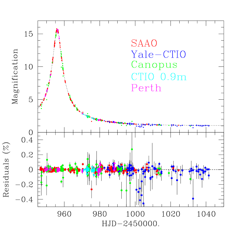
Figure 3.— Top Panel: The cleaned PLANET data for OGLE-1998-BUL-14. As in Figure 1, the magnification $A=(F-F_{\rm B})/F_{\rm S}$ is plotted. Only PLANET data prior to ${\rm HJD}^{\prime}=1050$, constituting $\sim 95\%$ of the complete PLANET data set are shown. The dashed line indicates the best-fit PSPL model, which has a time scale ${t_{\rm E}}=40$ days, and a minimum impact parameter $u_{0}=0.064$, corresponding to a maximum magnification of $A_{\rm max}\sim 16$. The entire data set consists of 461 $I$-band and 139 $V$-band data points, the majority of which was taken between ${\rm HJD}^{\prime}\simeq 950$ to ${\rm HJD}^{\prime}\simeq 1040$. The median sampling interval during this time span is about $1$ hour, or $10^{-3}{t_{\rm E}}$, with no gaps greater than four days. The data are from the Yale-CTIO 1m, South African Astronomical Observatory 1m, the Perth 0.6m, the Canopus 1m, and the CTIO 0.9m. Bottom Panel: Residuals from the best-fit PSPL model.

Figure 4.— The histograms show the distributions of the residuals of the individual data points from the best-fit PSPL model, divided by their respective errors, before correction for seeing and background systematics (dashed histogram) and after correction (solid histogram). The solid curve is a Gaussian of unit variance.

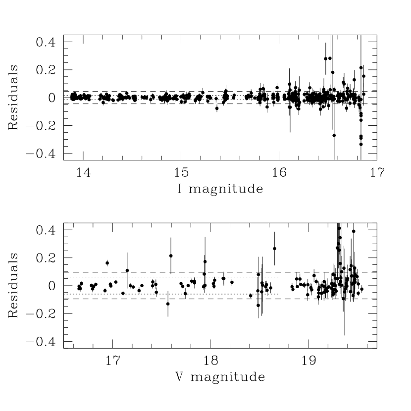
Figure 5.— The points with error bars are the residuals (in magnitudes) of the OGLE-1998-BUL-14 data points from the best-fit PSPL model as a function of the magnitude predicted by the model. We show the residuals separately for the $I$-band dataset (top panel) and the $V$-band dataset (bottom panel). The 1$\sigma$ scatter for the entire $I$-band data set, as denoted by the dashed line, is $\sim 4\%$, whereas the scatter for all points with $I<16$ is $1.5\%$ (dotted line). The 1$\sigma$ scatter for the $V$-band data set is $\sim 10\%$ (entire data set), and $\sim 7\%$ ($V<18.7$).

3. Observations

PLANET observations of OGLE-1998-BUL-14 were taken in two broad-band filters at five sites using seven different detectors. The five sites are the CTIO 0.9m and the Yale-CTIO 1m in Chile, the SAAO 1m in South Africa, the Canopus 1m in Tasmania, and the Perth 0.6m near Perth, Australia. Canopus data prior to ${\rm HJD}^{\prime}\equiv{\rm HJD}-2450000.0=975.0$ were taken with a different detector than those taken afterwards; we will refer to these data sets as Canopus A (${\rm HJD}^{\prime}<975.0$) and Canopus B (${\rm HJD}^{\prime}>975.0$), respectively. SAAO data were taken in three segments: during the period from ${\rm HJD}^{\prime}=976.0$ to ${\rm HJD}^{\prime}=980.0$, a different detector was used than prior to ${\rm HJD}^{\prime}=976.0$ or after ${\rm HJD}^{\prime}=980.0$, when the original detector was reinstalled on the telescope. Since different detectors have different characteristics that can affect the photometry, we will treat these as independent light curves. In addition, because the SAAO data prior to ${\rm HJD}^{\prime}=976.0$ and after ${\rm HJD}^{\prime}=980.0$ are substantially offset photometrically despite being taken with the same telescope, detector and filters, these are also treated as independent light curves. We refer to these as SAAO A (${\rm HJD}^{\prime}>976.0$), SAAO B ($976.0\leq{\rm HJD}^{\prime}\leq 980.0$) and SAAO C (${\rm HJD}^{\prime}\geq 980.0$). All independent light curves have both $I$ and $V$ band photometry, except for the CTIO 0.9m and Canopus B data, which do not have $V$-band photometry.

The entire data set consists of 461 $I$-band and 139 $V$-band data points forming a total of 14 independent light curves. The number of data points per light curve is given in Table 1. The data were reduced using DoPHOT (Schechter, Mateo, & Saha (1993)), and reference stars were chosen to optimize photometry at each individual site. For details concerning the reduction, see Albrow et al. (1998).

The PLANET data set for OGLE-1998-BUL-14 is one of the best sampled light curves to date. Over $95\%$ of the measurements were taken during a $3.3~{}{\rm month}$ time period from ${\rm HJD}^{\prime}=945.0$ to ${\rm HJD}^{\prime}=1045.0$, corresponding to times $-0.2{t_{\rm E}}$ before the peak until $2{t_{\rm E}}$ after the peak. In Figure 1, we show the distribution of sampling intervals (time between successive measurements) in hours for the cleaned PLANET OGLE-1998-BUL-14 dataset. The median sampling interval is about 1 hour, or $10^{-3}$ of the Einstein ring crossing time. Furthermore, there are very few gaps greater than 1 day.

Our primary results are based solely on PLANET data. We use the publically-available OGLE data set for OGLE-1998-BUL-14 only to test our PSPL model and to derive a parallax-based constraint on the lens mass. The OGLE data set consists of 159 data points taken in the standard $I$ filter with the 1.3 Warsaw Telescope in Chile: 125 baseline points were taken prior to ${\rm HJD}^{\prime}=800$ when the source was not being lensed, and the remaining 34 points taken during the course of the event. For more information on the OGLE project and the Early Warning System, which is used to alert microlensing events toward the Galactic bulge, see Udalski, Kubiak, & Szymański (1997), and Udalski et al. (1994).

4. Correcting for Known Systematic Effects

Along with the usual reduction procedures, we take additional steps to optimize the data quality before analyzing the light curve of OGLE-1998-BUL-14. Since planetary perturbations are expected to often have small amplitudes, it is essential that any low-level systematic deviations caused by observational effects be minimized in order to avoid spurious detections. Such effects can be quite common in crowded-field photometry. We describe in turn several systematic effects and our procedures to remove them.

Light curves of constant stars in our fields often display residuals from the mean value for the star that are correlated with seeing (or more specifically, image quality as measured by the FWHM of point sources), and occasionally with the sky background as well. These correlations seem to be a generic feature of crowded-field DoPHOT photometry, and presumably are present at some level in all light curves. We find that the magnitude (and sign) of the correlation depends on the site and detector, being quite strong for some data sets and almost completely absent in others. Typically, these correlations with the seeing and background are linear in flux and hence approximately linear in magnitudes, and are below 10%. Such correlations inflate the overall scatter in typical light curves by about a factor of two, diminishing the recognizability of subtle deviations. The correlation with FWHM can be especially dangerous: coherent deviations of order a few percent are seen on nightly time scales, partly due to the correlation between seeing and airmass. Such deviations can easily mimic low amplitude perturbations caused by small-mass planetary companions.

Based on studies of constant stars in crowded fields, Albrow et al. (1998) found that formal DoPHOT errors typically underestimate the true photometric uncertainties by a factor of $1.5-2$. Using the formal DoPHOT errors for our analysis would therefore overestimate the significance of any anomaly being studied. Furthermore, observed error distributions are not Gaussian, with long tails toward larger values, primarily due to the seeing and background systematics described above. These distributions are poorly represented by the formal DoPHOT errors. Thus, when not corrected for systematics, many light curves have more large ($>3\sigma$) outliers than would be expected from a Gaussian distribution. While it may be tempting simply to eliminate these outliers from the data set, such an approach could be dangerous since an isolated outlier could, in principle, be due to a short-duration deviation caused by a planetary companion. Unfortunately, in many cases the cause of the outliers is not known and nearly-simultaneous photometry that in principle could be used to discriminate real deviations from poor-quality data is not available.

Our approach is to apply a correction to the entire dataset prior to the analysis, as we now describe. We fit the entire data set to a preliminary PSPL model, including seeing and background correlation terms, so that for each observed light curve our model takes the form,

$$m_{{\rm pred},i}=m_{\rm PSPL}(t_{i})+\eta\theta_{i}+\zeta b_{i}.$$ (7)

Here $m_{{\rm pred},i}$ is the predicted flux in magnitudes, $m_{\rm PSPL}$ is the flux in magnitudes due to the PSPL magnification (Eq. 1) at time $t_{i}$, $\eta$ is the slope of the seeing correlation, $\theta_{i}$ is the DoPHOT-reported full-width half-maximum of the PSF of the $i$th data point, $\zeta$ is the slope of the correlation with background flux, and $b_{i}$ is the DoPHOT-reported background of the $i$th data point. In general, the specific model used to correct for seeing and background systematics is not important, provided that the model parameters are not strongly correlated with $\eta$ and $\zeta$. For most of the deviations we will be considering in this paper, i.e. those arising from nearly equal mass binary lenses, parallax, and finite source effects, model parameters are nearly uncorrelated with $\eta$ and $\zeta$. However, deviations caused by small mass ratio companions can occur over the course of several hours, and thus these deviations can be highly correlated with variations in seeing. Since these binary-lens models will not have the benefit of the additional fit parameters ($\eta,\zeta$), the significance of any short-duration deviation will be overestimated. We will return to this point in § 5.2.

We fit the model in the following way. We choose trial values for ${t_{\rm E}},u_{0}$, and $t_{0}$. This gives a prediction for the PSPL magnification as a function of time $A(t)$. The two parameters $F_{\rm S}$ and $F_{\rm B}$ are then determined by performing a linear fit to the flux. This gives the PSPL flux $m_{\rm PSPL}(t_{i})$. Finally, the parameters $\eta$ and $\zeta$ are determined by performing a linear fit in magnitudes. The final $\chi^{2}$ for the trial model with parameters (${t_{\rm E}},t_{0},u_{0},F_{\rm S},F_{\rm B},\eta,\zeta$) is then evaluated in magnitudes and the values of these parameters that minimize $\chi^{2}$ are then found using a downhill-simplex method (Press et al. (1992)). Using the final values of $\eta$ and $\zeta$, the data are corrected for the seeing and background systematics. This preliminary PSPL fit produces $\chi^{2}\sim 2000$ for 569 degrees-of-freedom (dof). Since no gross deviations from a PSPL light curve are apparent in the data, the high $\chi^{2}/{\rm dof}$ is an indication that the DoPHOT errors are underestimating the true error, in this case by a factor of $\sim 2$. Some of this inflated $\chi^{2}$ arises from a few highly-deviant outliers. Furthermore, different light curves have scatter that are underestimated by different amounts. For these reasons, simply scaling all the errors by a factor that forces $\chi^{2}/{\rm dof}$ to be unity would not be appropriate. We therefore adopt the following procedure. Using the preliminary model, we first find the largest $>3\sigma$ outlier and reject it. We recompute $\chi^{2}$ for each light curve, and then rescale the errors in the individual light curves by a factor that forces the $\chi^{2}/N_{i}$ for each light curve to be equal to unity, where $N_{i}$ is the number of measurements in light curve $i$. All the errors are then scaled with an overall factor to force $\chi^{2}/{\rm dof}$ for the entire data set to unity. This light curve is then refit to the model in equation (7), removing any residual seeing and background correlations. We iterate this process, successively removing the largest $3\sigma$ outlier, rescaling the errors, and refitting the light curve, until no further $3\sigma$ outliers remain, and the fit has converged. The final scaling factors are given in Table 1. We find a total of five outliers that deviate from the final model by more than $>3\sigma$. At the final step, we form two data sets. For the first data set, we reintroduce the $>3\sigma$ outliers, but with errors scaled by the same factor as their parent light curves; we will refer to this as the “cleaned” PLANET data set. The second data set does not contain the outliers; we refer to this as the “super-cleaned” PLANET data set. Finally, for some analyses, we combine the OGLE and super-cleaned PLANET data sets, scaling the OGLE errors by 2.01 so as to force $\chi^{2}/{\rm d.o.f.}$ to unity. We will refer to this as the OGLE+PLANET super-cleaned data set.

We now fit these corrected data sets to a PSPL model with parameters ${t_{\rm E}},t_{0},u_{0},F_{\rm S},F_{\rm B}$ (Eq. 1). For the PLANET datasets, there are 14 light curves, and thus the fit is a function of 31 parameters. Including OGLE data increases to the number of parameters by two. For the cleaned PLANET data set we find fit parameters and formal $1\sigma$ errors determined from the linearized covariance matrix of ${t_{\rm E}}=(39.6\pm 1.1)~{}{\rm days}$, $u_{0}=0.0643\pm 0.0002$, $t_{0}=956.016\pm 0.005$. The fit parameters for the super-cleaned PLANET data set and the OGLE+PLANET super-cleaned data set are the same within the errors. The parameters and formal $1\sigma$ errors for all three fits are summarized in Table 1, along with the blend fractions $g\equiv F_{\rm B}/F_{\rm S}$ for each light curve. The OGLE+PLANET dataset is shown in Figure 2, while the cleaned PLANET light curve and the best-fit PSPL model are shown in Figure 3, along with the residuals from the model.

In Figure 4 we show the distribution of residuals of the cleaned PLANET dataset from the best-fit PSPL model divided by their respective (rescaled) errors, along with a Gaussian of unit variance. Other than a few outliers, the two distributions are very similar, indicating that our errors are nearly Gaussian distributed. In order to illustrate the importance of including the seeing and background corrections, we also show the distribution of residuals divided by their respective rescaled errors before these corrections. The uncorrected data have a broader distribution with a median value that is systematically offset from zero; the entire distribution is highly non-Gaussian.

In Figure 5 we show the residuals of the cleaned PLANET dataset from the PSPL model as a function of the predicted magnitude of the model. The photometry in $I$ is excellent; the 1$\sigma$ scatter for $I<16$ is 1.5%; while the scatter for the entire $I$ dataset is $4\%$. The scatter is approximately 2.5 times larger in $V$; however this constitutes only $20\%$ of the entire dataset.

5. Limits on Companions to the Lens

The excellent coverage and high-quality photometry, combined with the fact that OGLE-1998-BUL-14 was a high-magnification event, make this an excellent candidate for the detection of planetary perturbations. Direct examination of the light curve and residuals reveals no obvious planetary signatures, and, in fact, no obvious deviations from the PSPL model of any kind. However, since the deviations could be quite subtle, it is important that the light curve be searched systematically for any deviations. If no significant deviations are found, the good photometry and excellent coverage can be used to place limits on the kinds of companions to the lens that could be present. To do this, we must calculate the detection efficiency of the OGLE-1998-BUL-14 light curve to companions.

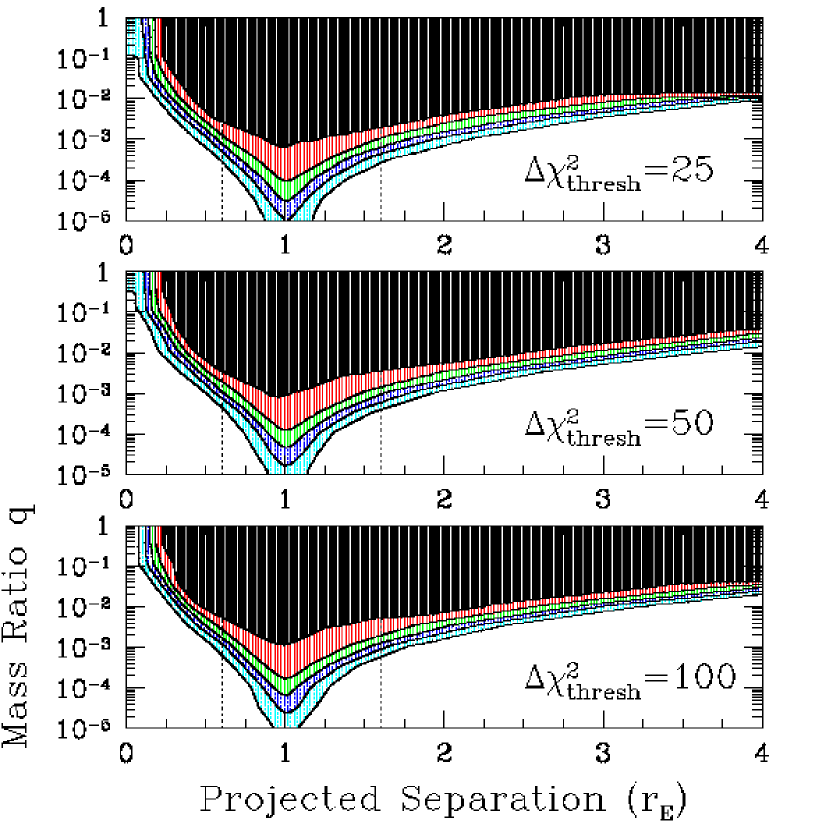
Figure 6.— The solid black lines are contours of constant detection efficiency, $\epsilon(d,q)$, for all PLANET OGLE-1998-BUL-14 data, shown for projected separations $d$ between the primary and companion in units of the Einstein ring radius, of $0<d<4$, and mass ratios between the primary and companion, $q$, of $0>\log(q)>-5.0$. The contours mark $\epsilon=5\%$ (outer contour), $25\%$, $50\%$, $75\%$, and $95\%$ (inner contour). The vertical dotted lines indicate the boundaries of the lensing zone, $0.6\leq d\leq 1.6$. The region of $(d,q)$ parameter space shaded in black is excluded by the observations at the $95\%$ confidence level. The panels are the results for different rejection criteria, $\Delta\chi^{2}_{\rm thresh}=25$ (top), $50$ (middle), $100$ (bottom). A mass ratio of $q=10^{-2}$ corresponds to the mass ratio between a $10M_{J}$ planet and a G dwarf. For this mass ratio, a companion with projected separation $0.4\leq d\leq 2.4$ is excluded at the 95% confidence level for all our rejection criterion. This corresponds to a range of instantaneous projected separations in physical units of 1.2 to 7.4 AU, assuming a G dwarf primary at 6.5 kpc.

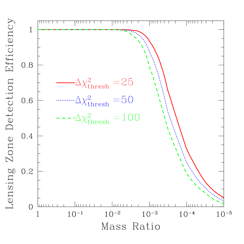
Figure 7.— The detection efficiency of PLANET OGLE-1998-BUL-14 data to a companion averaged over the lensing zone, $0.6\leq d\leq 1.6$, as a function of the mass ratio $q$ between the primary and the companion. We show the lensing zone detection efficiency for three different rejection thresholds, $\Delta\chi^{2}_{\rm thresh}=25$ (solid), $50$ (dotted), and $100$ (dashed).

5.1. Detection Efficiency of OGLE-1998-BUL-14 to Companions

The efficiency $\epsilon$ of a particular microlensing light curve to the detection of a binary system depends sensitively on two quantities: the the mass ratio of the system, $q$, and the angular separation $d$ in units of $\theta_{\rm E}$. The efficiency $\epsilon(d,q)$ tends to zero when $q\rightarrow 0$, $d\rightarrow 0$, or $d\rightarrow\infty$ (i.e. when the companion has a low mass compared to the primary, or is very close or very far from the primary). We simultaneously search for planetary deviations and calculate the detection efficiency for OGLE-1998-BUL-14 using a method proposed by Gaudi & Sackett (2000). We briefly review the steps below.

(1)

The OGLE-1998-BUL-14 light curve is fit with a PSPL model by minimizing $\chi^{2}$. The resulting $\chi^{2}$ for this model is labelled $\chi^{2}_{\rm PSPL}$.

(2)

Holding $d$ and $q$ fixed, the binary lens model that best fits the observed light curve is found for each source trajectory $\alpha$, leaving the 31 parameters (${t_{\rm E}},u_{0},t_{0},14\times F_{\rm S},14\times F_{\rm B}$) as free parameters. The difference $\Delta\chi^{2}(d,q,\alpha)\equiv\chi^{2}(d,q,\alpha)-\chi^{2}_{\rm PSPL}$ is evaluated.

(3a)

All parameter combinations ($d,q,\alpha$) yielding $\Delta\chi^{2}(d,q,\alpha)<\Delta\chi^{2}_{\rm flag}$ are flagged for further study as possible detections, where $\Delta\chi^{2}_{\rm flag}$ is some reasonable detection criterion.

(3b)

The fraction of all binary-lens fits for the given $(d,q)$ that satisfy the criterion $\Delta\chi^{2}>\Delta\chi^{2}_{\rm thresh}$ in computed, where $\Delta\chi^{2}_{\rm thresh}$ is a rejection criterion. The detection efficiency $\epsilon(d,q)$ of the data set for the assumed separation and mass ratio,

$$\epsilon(d,q)\equiv{1\over 2\pi}\int_{0}^{2\pi}{\rm d}\alpha\,\,\Theta[\Delta\chi^{2}(d,q,\alpha)-\Delta\chi^{2}_{\rm thresh}],$$ (8)

where $\Theta[x]$ is a step function, is then computed. Note that $\alpha$ is uniformly distributed.

(4)

Items (2) and (3) are repeated for a grid of $(d,q)$ values. This gives the detection efficiency $\epsilon(d,q)$ for OGLE-1998-BUL-14 as a function of $d$ and $q$, and also all binary-lens parameters $(d,q,\alpha)$ that give rise to significantly better fits to the light curve than the PSPL model.

(5)

The parameter combinations found in step (3a) are then used as initial guesses for our binary-lens $\chi^{2}$ minimization routine, leaving all 34 parameters as free parameters, in order to find the minimum $\chi^{2}$ and best-fit parameters for this local minimum.

We search for binary-lens fits and calculate $\epsilon(d,q)$ for $0\leq d\leq 4$ and $0\geq\log(q)\geq-5$ at intervals of $0.1$ in $d$ and $0.5$ in $\log(q)$. Since the search is performed on a grid of ($d,q,\alpha$) and the grid points are unlikely to be situated exactly on local minima, it important that $|\Delta\chi^{2}_{\rm flag}|$ be sufficiently low so that all probable fits are found. We chose $\Delta\chi^{2}_{\rm flag}=-9$ for our flagging criterion, and find only three combinations of $d$ and $q$ for which $\Delta\chi^{2}<\Delta\chi^{2}_{\rm flag}$. Minimizing $\chi^{2}$ in the neighborhood of these trial solutions reveals that the best-fit parameters are quite close to the initial parameters, and $\chi^{2}$ decreases minimally. The absolute best-fit binary lens to OGLE-1998-BUL-14 has a $\chi^{2}=720.6$, or $\Delta\chi^{2}=-9.2$. Since this is well below our threshold for detection of $\Delta\chi^{2}=-50$, we do not claim a detection. Indeed, even a naive calculation based on Gaussian statistics and three additional parameters to describe the companion yields a chance probability of 2.7% for $\Delta\chi^{2}\leq-9.2$, which cannot be considered a detection at even the 3-sigma level.

In fact, the probability of a random fluctuation of this magnitude is substantially higher than 2.7%. First, since we are including outlier points in the search, $\chi^{2}$ should be renormalized by the number of degrees of freedom, which would imply $\Delta\chi^{2}=-7.2$ for which the chance probability with three additional parameters is 6.7%. However, the chance probability of a false planet detection is substantially higher than this. Moreover, it cannot be computed from a $\chi^{2}$ table and would have to be determined by Monte Carlo simulation. To understand why, consider one of the planetary models we found that fits OGLE-1998-BUL-14 with $\Delta\chi^{2}=-7.2$. The “success” of this model is basically driven by 15 points clustered within 1 day whose mean lies $\sim 0.6\%$ above the PSPL model. The chance for such a deviation on this particular day is $\sim\exp(\Delta\chi^{2}/2)/(2\pi|\Delta\chi^{2}|)^{1/2}=0.4\%$. Since there are a total of $\sim 600$ data points, there is a similar probability for such a fluctuation on each of $600/15=40$ time intervals. Hence, the total probability is $1-(1-0.004)^{40}\sim 15\%$. In fact, the probability is somewhat higher still because we have taken account of only 15-point clusters and not larger or smaller clusters that could also mimic a planet.

In any event, we have set our detection threshold substantially higher than would be warranted solely to avoid chance statistical fluctuations. This conservative approach is motivated by concern over unrecognized systematics which, experience has taught us, often give rise to spurious detections of formally high significance. We therefore conclude that the light curve of OGLE-1998-BUL-14 is consistent with a single lens within the uncertainties.

5.2. Resulting Constraints on Companions

The detection efficiency at a given $(d,q)$ is the probability that a companion of separation $d$ and mass ratio $q$ would have produced a deviation inconsistent (in the sense of $\Delta\chi^{2}>\Delta\chi^{2}_{\rm thresh}$) with the observed OGLE-1998-BUL-14 light curve. If no deviations are seen, companions with ($d,q$) can be ruled out at a confidence level of $\epsilon(d,q)$. The choice of the rejection threshold $\Delta\chi^{2}_{\rm thresh}$ can have a significant effect on the resulting detection efficiency, especially for low thresholds and mass ratios $q{{}_{<}\atop{}^{{}^{\sim}}}10^{-3}$ (Gaudi & Sackett (2000)). We choose to be conservative, and adopt $\Delta\chi^{2}_{\rm thresh}=50$ as our fiducial threshold. For comparison, we also show the results for $\Delta\chi^{2}_{\rm thresh}=25$ and $\Delta\chi^{2}_{\rm thresh}=100$.

The binary-lens detection efficiency of OGLE-1998-BUL-14 as a function of the mass ratio $q$ and angular separation $d$ is shown in Figure 6. The darkest shading denotes those parameter combinations $(d,q)$ for which $\epsilon>95\%$, and thus are excluded at the $95\%$ confidence level from lying above the rejection criterion. Table 2 shows the range of angular separations $d$ that are excluded by our OGLE-1998-BUL-14 data set for several mass ratios and the three different rejection thresholds, $\Delta\chi^{2}_{\rm thresh}=25,50$, and $100$. For $q{{}_{>}\atop{}^{{}^{\sim}}}10^{-1.5}$, $\epsilon=100\%$ out to the largest separation for which we calculate $\epsilon$, namely $d=4.0$. For these mass ratios $d=4$ is thus a lower limit to the excluded range; the upper end of the excluded range is likely to be considerably larger. We find that any companion to the primary lens with mass ratio $q{{}_{>}\atop{}^{{}^{\sim}}}10^{-2}$ and angular separation $0.4\leq d\leq 2.4$ is excluded by the data, that is, such a companion would produce deviations at the $\Delta\chi^{2}>100$ level that are not observed.

Note that these limits apply to individual companions only, not to systems of companions. Implicit in our calculation of $\epsilon(d,q)$ is the assumption that multiple planets affect the magnification structure of the lens, and therefore the deviation from the single-lens magnification, in an independent way. This assumption is likely to break down in regions near the central caustic when more than one planet is in the lensing zone (Gaudi, Naber, & Sackett (1998)). In this case, the efficiencies calculated using the method of Gaudi & Sackett (2000) will be in error by an amount that will depend on the relative mass ratios, orientations, and projected separations of the two companions. Since OGLE-1998-BUL-14 is a high-magnification event, and most of the constraints come from portions of the light curve near the peak of the event (i.e. where the central caustic is probed), our results are only strictly valid for single planets. A full investigation of the effect of multiple planets of $\epsilon$ is beyond the scope of this paper. We expect, however, that the planet detection efficiencies for multiple Jovian planetary systems may actually be higher than for single planets near the peak of OGLE-1998-BUL-14, since the region of anomalous magnification near the central caustic generally occupies a larger fraction of the Einstein ring when two planets are present (Gaudi, Naber, & Sackett (1998)).

It is interesting to compare the limits on companions to the primary lens of OGLE-1998-BUL-14 to those for the primary lens of MACHO-98-BLG-35 derived by the MPS/MOA collaborations (Rhie et al. 1999b ). MACHO-98-BLG-35 was a higher magnification event $(A_{\rm max}\sim 75)$ than OGLE-1998-BUL-14 $(A_{\rm max}\sim 16)$. Since higher magnification events have higher intrinsic detection efficiencies (Griest & Safizadeh (1998); Gaudi & Sackett (2000)), one would expect, for similar sampling and photometric precision, the limits on companions to be more stringent for MACHO-98-BLG-35. However, although the photometric precision obtained by MPS/MOA on MACHO-98-BLG-35 is similar to that for OGLE-1998-BUL-14 ($\sim$ few percent), the sampling of MACHO-98-BLG-35 (in terms of fraction of the time scale ${t_{\rm E}}$) is poorer, due primarily to the fact that MACHO-98-BLG-35 was a shorter time scale event. Although Rhie et al. (1999b) used a slightly different method to calculate $\epsilon(d,q)$ than that suggested by Gaudi & Sackett (2000), and used a different rejection criterion ($\Delta\chi^{2}_{\rm thresh}=40$), we can make a rough comparison between their resulting detection efficiencies shown in their Fig. 7 with ours for $\Delta\chi^{2}_{\rm thresh}=50$ shown in the middle panel of Fig. 6. We see that the detection efficiencies to companions are everywhere higher for MACHO-98-BLG-35 than for OGLE-1998-BUL-14. This indicates that, when the peak of the event can be measured, maximum magnification is a more important factor than sampling in determining the constraining power (and hence the ability to detect companions) in an observed microlensing event.

In Figure 7 we show the detection efficiency averaged over the lensing zone (where the detection efficiency is the highest), $0.6\leq d\leq 1.6$,

$${\epsilon}_{\rm LZ}(q)\equiv\int_{0.6}^{1.6}\epsilon(d,q)~{}{\rm d}d~{},$$ (9)

for mass ratios $0\leq q\leq 10^{-5}$. The lensing zone detection efficiencies for several representative mass ratios are tabulated in Table 3. For a planetary model in which companions have angular separations distributed uniformly throughout the lensing zone, ${\epsilon}_{\rm LZ}$ represents the probability that a companion of mass ratio $q$ would have been detected with the OGLE-1998-BUL-14 data set. These probabilities are quite high: for example, the detection efficiency for a companion of mass ratio $q{{}_{>}\atop{}^{{}^{\sim}}}10^{-3}$ in the lensing zone of the OGLE-1998-BUL-14 primary is ${{}_{>}\atop{}^{{}^{\sim}}}80\%$.

For this analysis, we have assumed that the source can be treated as point-like. Finite source effects will have a substantial effect on $\epsilon(d,q)$ if the angular size of source $\rho_{*}\equiv\theta_{*}/\theta_{\rm E}$ is comparable to the Einstein ring radius of the companion, $\theta_{\rm p}=\theta_{\rm E}q^{1/2}$ (Gaudi & Sackett (2000)). Any planetary deviations will be broadened but reduced in amplitude for $\rho_{*}{{}_{>}\atop{}^{{}^{\sim}}}q^{1/2}$. For OGLE-1998-BUL-14, no finite source size effects were detected, thus we can place an upper limit on $\rho_{*}$. As we show in the § 6.2, the $3\sigma$ limit is $\rho_{*}\leq 0.062~{}$. Thus the detection efficiencies calculated above are strictly valid only for $q{{}_{>}\atop{}^{{}^{\sim}}}10^{-2.5}$. However, for typical lens parameters, $\rho_{*}$ is likely to be considerably smaller, $\rho_{*}\sim 0.01$. Statistically, we thus expect the results to be valid for $q{{}_{>}\atop{}^{{}^{\sim}}}10^{-4}$. For mass ratios less than this, the detection efficiencies calculating using a point source may be overestimated by tens of percent (Gaudi & Sackett (2000)).

Poorly-constrained blend fractions can also induce substantial uncertainties in the derived detection efficiencies, due to the correlation between blending and impact parameter $u_{0}$ (Gaudi & Sackett (2000)). Fortunately, blending is easier to constrain in high-magnification events. Indeed, due to the high magnification of OGLE-1998-BUL-14 and the dense and precise photometry, the blend fraction of the event, and therefore $u_{0}$, are quite well constrained. The fractional error in $u_{0}$ is $<1\%$ and should contribute negligibly to the uncertainty in $\epsilon(d,q)$.

When fitting for the binary-lens model, we did not include seeing and background correlation terms (§ 4). Although the proper approach would be to include these terms in all binary-lens fits (and indeed, all fits in general), the computational cost is prohibitive. Since these terms were included in the PSPL fit, this implies that $\Delta\chi^{2}$ between the binary-lens fit and single-lens fit may be overestimated if the deviations from the PSPL fit due to the binary lens are highly correlated with either the seeing or background. This is generally not a problem for background correlations because the systematic deviations arising from the long time scale changes in the background are unlikely to be confused with deviations caused by companions. However seeing correlations are more insidious, because the short-time scale deviations caused by low mass ratio companions could be confused with systematic deviations arising from the nightly seeing changes in a poorly sampled light curve. Consider a deviation from the PSPL light curve that is perfectly correlated with the seeing. It can be shown that the fractional error in $\chi^{2}$ one makes by not including the seeing correlation in the binary lens fit is $\Delta\chi^{2}/\chi^{2}\sim N_{\delta}/N_{\rm tot}$, where $N_{\delta}$ is the number of deviant data points and $N_{\rm tot}$ is the total number of data points in the light curve. For uniformly sampled data, this is simply the ratio of the time scale of the perturbation $t_{\delta}$ to the total duration of observations. For planetary microlensing, $t_{\delta}\sim q^{1/2}{t_{\rm E}}$, and thus $\Delta\chi^{2}/\chi^{2}\sim q^{1/2}$. Thus for small mass ratios, $q<10^{-3}$, the fractional error in $\chi^{2}$ is small ${{}_{<}\atop{}^{{}^{\sim}}}3\%$. For $q>10^{-3}$, the companions produce coherent deviations that last many days, and thus cannot be correlated with the seeing. We therefore conclude that neglecting the seeing and background correlations does not result in seriously overestimated detection efficiencies.

Figure 8.— Excluded regions for the lens mass and distance based on the lack of second-order signatures in the light curve of OGLE-1998-BUL-14. The solid lines show $3\sigma$ upper or lower limits to the mass of the lens in solar masses $M/M_{\odot}$ as a function of the distance of the lens in ${\rm kpc}$ for a source distance of $8~{}{\rm kpc}$. The solid hatching shows the excluded region from the lack of parallax effects. The short-dashed hatching shows the region excluded by the lack of finite source effects. Combining the finite source and parallax limits, we obtain a lower limit to the mass, which is shown as the triangle. The long-dashed hatching shows the region excluded if the lens is a main-sequence star; the upper limit to the lens mass is shown as a cross. The dotted horizontal line is the hydrogen-burning limit. Our adopted lens mass $M=M_{\odot}$ and distance $D_{\rm L}=8~{}{\rm kpc}$ are shown as the square.

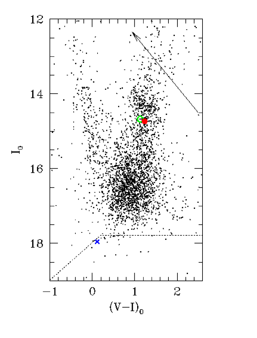
Figure 9.— Calibrated, dereddened color-magnitude diagram for the field centered on OGLE-1998-BUL-14 from Yale-CTIO 1m data. The mean reddening for the field is $A_{I}$ and E$(V-I)$=1.56, determined from the mean $I$ magnitude and $V-I$ color of the clump. The arrow shows the direction and magnitude of the dereddening vector. The open circle shows the dereddened position of the unmagnified source, which is composed of the microlensed source (filled circle) and an unresolved blended star (cross). The dotted line shows the $3\sigma$ upper limit to the dereddened I magnitude of the lens, assuming the extinction to the lens is the same as the OGLE-1998-BUL-14 field.

6. Limits on the Mass of the Lens

In the previous section, we placed limits on possible companions to the primary lens responsible for the microlensing event OGLE-1998-BUL-14 by calculating the detection efficiency as a function of the mass ratio $q$ and angular separation $d$ between the primary and secondary in units of the angular Einstein ring of the system. Although limits on the mass ratio are interesting in their own right, what is of interest ultimately are limits on the mass of the companion, $M_{\rm p}$, and the physical orbital separation of the companion, $a$. In order to translate limits on $q$ and $d$ into limits on $M_{\rm p}$ and $a$, one must know the mass of the primary lens, $M$, and its distance $D_{\rm L}$, and the orbital phase and inclination of the system.

Unfortunately it is not generally possible to measure the mass and distance to the lens. The only parameter one can measure from a generic single lens event that contains information about the lens is the time scale ${t_{\rm E}}$, a degenerate combination of the mass $M$, distance $D_{\rm L}$, and transverse velocity $v$ of the lens (c.f. Eq. 6). However, detection of various higher order effects, such as parallax or finite source effects, enables one to extract additional information and partially break this degeneracy. In the following subsections, we search for signatures of these effects in the light curve of OGLE-1998-BUL-14. Other than a marginal detection of a parallax asymmetry, we do not detect either of these effects, and use their absence to exclude regions of the $(M,D_{\rm L})$ plane. In addition, we place a limit on the amount of light emitted from the lens itself, and translate this into a limit on the lens mass. As we show, despite the excellent photometry and coverage of OGLE-1998-BUL-14, the limits on these higher order effects are not very stringent, and do not translate into strong constraints on the mass of the lens.

The analysis uses the super-cleaned PLANET data set since, as opposed to planetary perturbations, the effects we are searching for here induce subtle deviations with time scales of many days, and therefore cannot be described by a isolated large outliers. Using the super-cleaned data set (which does not include these outliers) will provide more robust and reliable limits. For the parallax analysis only we use the OGLE+PLANET cleaned data set in order to have a more secure description of the total baseline flux.

6.1. Parallax Limits

The motion of the Earth around the Sun induces departures from rectilinear motion in the path of the lens relative to the Earth-source line-of-sight and thus alters the formula for the angular separation $u(t)$ as a function of time. This phenomenon is commonly referred to as parallax, and in general gives rise to light curves that deviate from the standard PSPL model (Gould (1992); Alcock et al. (1995)). The magnitude of the deviation depends on the time of year when the event peaks, the angle $\phi$ of the lens trajectory with respect to the north ecliptic pole, and the transverse velocity ${\bf\tilde{v}}\equiv{\bf v}(D_{\rm S}/D_{\rm LS})$ of the lens projected onto the observer plane.

If the time scale of the event is short compared to the period of the Earth’s orbit, the Earth’s acceleration can be approximated as constant over the course of the event. In this case, the angular separation can be written as (Gould, Miralda-Escudé, & Bahcall (1994)),

$$u(t)=\left[\xi^{2}+u^{2}_{0}\right]^{1/2},~{}~{}~{}~{}\xi\equiv\tau+{1\over 2}\kappa{t_{\rm E}}\tau^{2},$$ (10)

where $\tau\equiv(t-t_{0})/{t_{\rm E}}$. The asymmetry parameter $\kappa$ is given by,

$$\kappa=\Omega_{\oplus}{v_{\oplus}\over\tilde{v}}\sin\lambda\sin\phi,$$ (11)

where $\Omega_{\oplus}=2\pi~{}{\rm yr}^{-1}$, $v_{\oplus}\simeq 30~{}{\rm km}\,{\rm s}^{-1}$ is the linear speed of the Earth around the Sun, and $\lambda$ is the angle between the source and Sun at the time of maximum magnification. In the case of OGLE-1998-BUL-14, $\sin\lambda\sim 0.5$. Implicit in equation (11) is the approximation that the source is in the Galactic plane. Thus, for short-time scale events one can measure only the degenerate combination $\tilde{v}/\sin\phi$.

We fit our OGLE-1998-BUL-14 light curve data with the parallax asymmetry model above and find an improvement of $\Delta\chi^{2}=4.4$ for 1 extra dof over the standard PSPL model, corresponding to a $\sim 2\sigma$ detection of an asymmetry. We find a best-fit value of $\kappa=6.1\pm 3.6\times 10^{-4}~{}(1\sigma)$, corresponding to

$${\tilde{v}\over\sin{\phi}}=(420\pm 250)~{}{\rm km}\,{\rm s}^{-1}~{}~{}~{}(1\sigma).$$ (12)

This detection is not particularly useful for our purposes, however, not only because it is merely a $2\sigma$ detection, but also because the direction of lens motion is unknown.

In order to obtain a constraint on $\tilde{v}$ that is independent of $\phi$, we must use the form for $u(t)$ that includes the full two-dimensional ($\tilde{v},\phi$) parallax information (Alcock et al. (1995)). Given that the detection of asymmetry was marginal, it is not surprising that we are unable to obtain independent constraints on $\tilde{v}$ and $\phi$. Calculating $\chi^{2}$ as a function of $\tilde{v}$, and letting all other parameters (including $\phi$) vary, we recover the detection of the parallax asymmetry for $\tilde{v}{{}_{>}\atop{}^{{}^{\sim}}}30~{}{\rm km}\,{\rm s}^{-1}$. For $\tilde{v}{{}_{<}\atop{}^{{}^{\sim}}}30~{}{\rm km}\,{\rm s}^{-1}$, however, $\tilde{v}$ becomes comparable to the Earth’s velocity. For these small velocities, the component of the Earth’s velocity perpendicular to the motion of the lens becomes significant, and the light curve begins to deviate appreciably from the PSPL model, in a manner that is inconsistent with the observations for all values of $\phi$. This produces a lower limit to the projected velocity that is independent of $\phi$,

$$\tilde{v}>28.5~{}{\rm km}\,{\rm s}^{-1}~{}~{}~{}~{}{\rm(3\sigma)}.$$ (13)

We can combine this limit with the time scale of the event to give a lower limit to the lens mass as a function of the relative lens distance,

$$M(x)>6.7\times 10^{-3}M_{\odot}{{1-x}\over x}~{}~{}~{}~{}{\rm(Parallax,3\sigma)}$$ (14)

where $x\equiv D_{\rm L}/D_{\rm S}$. This limit is shown in Figure 8.

For bulge self-lensing, both lens and source belong to a population with approximately isotropic velocity distributions, producing no preferred direction for the transverse velocity, $v$, and thus no preferred value for $\phi$. For disk lenses, however, there is a preferred direction for $\phi$ due to Galactic rotation, in which case we would obtain a stronger limit on $\tilde{v}$. Unfortunately, we do not know a priori whether the lens is in the bulge or disk. We will therefore adopt the conservative assumption that there is no preferred direction for $v$, and use the limit given in equation (14).

6.2. Finite Source Limit

A point-lens transiting the face of a source will resolve it, creating a distortion in the magnification that deviates from the form given in equation (2). A detection of this distortion gives a measurement of the angular size of the source, $\theta_{*}$, in units of the angular Einstein ring radius, $\rho_{*}=\theta_{*}/\theta_{\rm E}$ (Gould (1994); Nemiroff & Wickramasinghe (1994); Witt & Mao (1994)). The requirement for such finite source effects to be detectable is that the impact parameter of the event must be comparable to or smaller than the dimensionless source size, $u_{0}{{}_{<}\atop{}^{{}^{\sim}}}\rho_{*}$. No such finite-source deviations are apparent in the light curve of OGLE-1998-BUL-14. This implies an upper limit to the dimensionless source size of $\rho_{*}{{}_{<}\atop{}^{{}^{\sim}}}0.06$. For a more exact limit, we calculate $\chi^{2}$ as a function of $\rho_{*}$, leaving all other parameters free to vary, and find that

$$\rho_{*}<0.062~{}~{}~{}(3\sigma).$$ (15)

In calculating this limit, we have assumed a uniform surface brightness profile for the source. Using a more realistic, but model-dependent, limb-darkened profile weakens this limit slightly.

In order to convert this upper limit on $\rho_{*}$ into a lower limit on $\theta_{\rm E}$, we must know the angular size of the source, $\theta_{*}$, which can be estimated from its $(V-I)$ color and $I$ magnitude. Figure 9 shows the calibrated dereddened color magnitude diagram (CMD) for OGLE-1998-BUL-14 field from Yale-CTIO 1m data. The stars in the OGLE-1998-BUL-14 field were calibrated relative to observations of 9 standard stars in Landolt (1992), measured several times during the night of 14 August 1998 at the Yale-CTIO 1m telescope in the same $V$ and $I$ filters used for the observations of the microlensing event. Extinction and color correction terms were derived in the normal manner. Comparison with similar measurements on other nights suggests the accuracy of the calibration is $\sim 0.02$ mag. We fit the distribution of $I$ magnitudes and $(V-I)$ colors of the observed clump to the model of Stanek (1995). We then determined the ${\rm E}(V-I)$ and $A_{I}$ by comparing our fitted clump magnitude and color to the dereddened $I_{\rm cl,0}$ and $(V-I)_{\rm cl,0}$ of the clump for the bulge as determined by Paczyński & Stanek (1998). We find ${\rm E}(V-I)=1.56$ and $A_{I}=2.16$. Using the PSPL fit and Yale-CTIO standards, we determine the calibrated, dereddened color and magnitude of the microlensed source to be $I_{0}=14.73\pm 0.03$ and $(V-I)_{0}=1.23\pm 0.08$, where the errors reflect the calibration and model uncertainties added in quadrature. From its position on the CMD, Figure 9, we conclude that OGLE-1998-BUL-14 is likely to be a clump giant or a RGB star.

To obtain an estimate of the source radius, $\theta_{*}$, we use the empirical color-surface brightness relationship for giant stars derived by van Belle (1999), which we rewrite as

$$\theta_{*}=6.0~{}\mu{\rm as}~{}10^{-0.2(V-16)+0.5[(V-I)-1.2]},$$ (16)

where we have assumed the relationship $(V-K)=2.2(V-I)$, derived from Bertelli et al. (1994) isochrones. For our parameters, we find $\theta_{*}=6.3\mu{\rm as}$. An uncertainty in the extinction $\delta A_{\rm V}$ leads to an uncertainty in the angular size of $\delta\theta_{*}/\theta_{*}\sim-0.16~{}\delta A_{\rm V}$, where the coefficient depends on the temperature of the source (Albrow et al. (1999)), which we have assumed to be $T=5000~{}{\rm K}$. We estimate the uncertainty in the extinction to be $\delta A_{\rm V}\sim 0.15$, based on the dispersion of the clump, resulting in an uncertainty of $\sim 2\%$ in $\theta_{*}$. The $3\%$ uncertainty in the $I$-magnitude of the source leads to an additional uncertainty of $\sim 1\%$ in $\theta_{*}$; the $8\%$ uncertainty in the color leads to an uncertainty of $\sim 6\%$ in $\theta_{*}$. Adding these in quadrature, we find $\theta_{*}=(6.3\pm 0.4)~{}\mu{\rm as}$.

Adopting this value for the angular size of the source, we can now translate the limit on $\rho_{*}$ (Eq. 15) directly to a limit on the angular Einstein ring radius,

$$\theta_{\rm E}>100~{}\mu{\rm as}~{}~{}~{}~{}(3\sigma).$$ (17)

Since $\theta_{\rm E}$ depends only on the lens mass and distance and on the distance to the source, this limit can be written in terms of a limit of the lens mass as a function of the relative lens distance,

$$M(x)>1.0\times 10^{-2}M_{\odot}{x\over{1-x}}~{}~{}~{}~{}{\rm(Finite~{}Source,3\sigma)}$$ (18)

We combine the parallax limit (Eq. 14) and the finite source limit (Eq. 18) to obtain a lower limit to the lens mass $M>8.3\times 10^{-3}M_{\odot}$, which occurs at $x=3.55$. This lower limit is indicated in Figure 8.

6.3. Luminous Lens Limit

If the lens of OGLE-1998-BUL-14 is a main-sequence star, it emits light. Although the angular separation between the lens and source is much too small for the lens to be resolved, additional light from the lens could, in principle, alter the shape of the light curve (c.f. Eq. 1). For most microlensing events, degeneracies between the fit parameters make it difficult to constrain accurately the amount of blended light, and thus any light that may be arising from the lens itself. Fortunately, the good photometry, complete coverage, and small $u_{0}$ of OGLE-1998-BUL-14 enable the blend fraction to be constrained quite tightly, allowing us to place an interesting upper limit on the blended light emitted by the lens.

To do this, we rewrite the flux of any unresolved light as $F_{\rm B}=F_{\rm U}+F_{\rm L}$, where $F_{\rm L}$ is the flux of the lens, and $F_{\rm U}$ is the flux of any additional unresolved source. Equation 1 is then

$$F(t)=F_{\rm S}A(t)+F_{\rm U}+F_{\rm L}.$$ (19)

We assume that the $I$-band flux of the lens is the same for all the $I$-band light curves, and similarly that the $V$-band flux is the same for all the $V$-band light curves. This is a reasonable assumption, since all the observatories use the same $I$ and $V$ filters, and because the lens and source will be unresolved for all observatories. However, due to differences in pixel size and image quality, we must allow additional unresolved light, $F_{\rm U}$ not associated with the lens or source to vary from site to site. We then compute $\chi^{2}$ as a function of $F_{\rm L}$, allowing the other parameters to vary, and imposing the constraint that $F_{\rm B}$ always be positive. For $F_{\rm L}\ll F_{\rm S}$, $\Delta\chi^{2}$ between the fit with and without a luminous lens is small. However, as $F_{\rm L}$ increases, $\Delta\chi^{2}$ rises because $F_{\rm U}$ must be negative to match the observations, which is unphysical. In this way we find the minimum $I$-band magnitude of the lens that is consistent with our observations to be

$$I_{\rm L}>\cases{21.69-(V-I)&if $(V-I)\leq 1.75$\cr 19.94&if $(V-I)\geq 1.75$\cr},$$ (20)

where the limit is $3\sigma$. Note that this limit is not dereddened since the lens may have less extinction than the mean extinction toward the OGLE-1998-BUL-14 field. For reference, the dereddened limit is shown in Figure 9, assuming the reddening to the lens is the same as for the OGLE-1998-BUL-14 field.

In order to convert this limit on lens light into a limit on the lens mass as a function of its distance, we must adopt a relationship between mass and $I$ and $V$ magnitude. For this purpose, we use the solar metallicity Bertelli et al. (1994) theoretical isochrones for $M>0.6~{}M_{\odot}$, the solar metallicity Yale isochrones (Demarque et al. (1996)) for $0.35~{}M_{\odot}\leq M\leq 0.6~{}M_{\odot}$, and extrapolate the Yale isochrones using a 2nd order polynomial for $0\leq M\leq 0.35~{}M_{\odot}$. We assume that the dust is distributed uniformly between the observer and $1.5~{}{\rm kpc}$, with a total reddening at $1.5~{}{\rm kpc}$ equal to the mean reddening of the OGLE-1998-BUL-14 field, ${\rm E}(V-I)=1.56$ and $A_{I}=2.16$. For all distances between 0 and $8~{}{\rm kpc}$, we find the largest mass that is consistent with the apparent magnitude limit (Eq. 20). This mass-distance limit is shown in Figure 8. It can be adequately represented by,

$$\log[M(x)]<0.8+0.07x-0.75x^{-0.2}~{}~{}~{}~{}{\rm(Luminous~{}Lens,3\sigma)}$$ (21)

Varying the age, metallicity, or dust distribution within reasonable limits changes the mass limit at any distance by ${{}_{<}\atop{}^{{}^{\sim}}}0.2$ dex.

If the lens is a main-sequence star, the largest mass consistent with the lack of appreciable light in the light curve of OGLE-1998-BUL-14 is $M\sim 1.3~{}M_{\odot}$ which occurs when $D_{\rm L}\sim 8~{}{\rm kpc}~{}(x=1)$. Thus the lens must be a G dwarf or later. Of course, the lens may not be a main sequence star. Gould (1999) estimates that $\sim 80\%$ of events detected toward the bulge are due to main-sequence lenses. The remaining $20\%$ are due to stellar remnants, i.e. as white dwarfs, neutron stars, or black holes. If the lens is such a remnant, it would not obey the mass-luminosity relationship used to find the limit in equation (21). However, white dwarfs and neutron stars have masses of $M_{\rm WD}\sim 0.6~{}M_{\odot}$ and $M_{\rm NS}\sim 1.35~{}M_{\odot}$, and so automatically satisfy this limit for nearly all likely distances to the lens. Thus the vast majority (99%) of lenses will satisfy the limit in equation (21).

6.4. Combined Limits

The limits on the mass and distance to the lens set in the previous subsections are, for the most part, model independent. Unfortunately, they are also not very stringent. Even with the assumption that the lens is a main-sequence star, the allowed regions in the $(M,D_{\rm L})$ plane are quite large, spanning two orders of magnitude in mass, $0.01~{}M_{\odot}{{}_{<}\atop{}^{{}^{\sim}}}M{{}_{<}\atop{}^{{}^{\sim}}}1.3~{}M_{\odot}$, and nearly the entire range in distance, $0.5~{}{\rm kpc}{{}_{<}\atop{}^{{}^{\sim}}}D_{\rm L}{{}_{<}\atop{}^{{}^{\sim}}}8~{}{\rm kpc}$. Our analysis indicates that, even with excellent coverage and good photometry, it will be quite difficult to routinely obtain stringent limits on the mass and distance to the lens for most events based on photometry alone.

It has been shown by Dominik (1998) how probability densities for physical quantities of the lens system can be derived under the assumption of statistical distributions of the mass spectrum, the mass density, and the transverse velocity. Rather than doing this, we will simply note that if the lens is in the bulge ($6~{}{\rm kpc}{{}_{<}\atop{}^{{}^{\sim}}}D_{\rm L}{{}_{<}\atop{}^{{}^{\sim}}}8~{}{\rm kpc}$), and has a typical transverse velocity for bulge self-lensing events ($v\sim 100~{}{\rm km}\,{\rm s}^{-1}$), then the measured ${t_{\rm E}}$ implies that it is likely to have a mass near the upper end of the allowed range. However, we cannot rule out that the lens is moving slowly, and therefore that the mass is quite small.

7. Discussion

7.1. The Detection Efficiency as a Function of Mass and Separation

In order to convert the limits on companions in the $q-d$ plane to limits on companions in the $M_{\rm p}-a$ plane, we need estimates of the mass and distance to the lens. However, as we demonstrated in § 6, it is quite difficult to obtain stringent limits on these quantities from photometric data alone. For illustrative purposes, therefore, we will simply assume that the lens is a G dwarf and adopt $M=M_{\odot}$, and a lens distance of $6.5~{}{\rm kpc}$, so that ${r_{\rm E}}=3.1$ AU. We stress, however, that this choice is somewhat arbitrary, and that the lens mass may be smaller by two orders of magnitude.

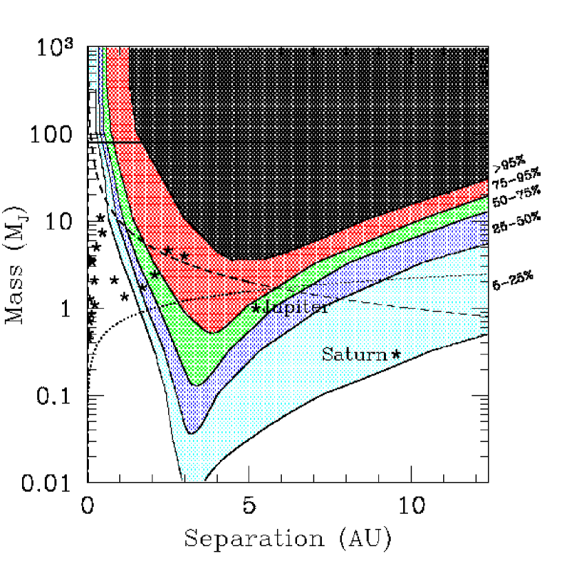
Figure 10.— Example detection efficiencies for the PLANET data set of OGLE-1998-BUL-14 as a function of the mass and orbital separation of the companion assuming a primary lens mass of $M_{\odot}$ and Einstein ring radius of ${r_{\rm E}}=3.1~{}{\rm AU}$. The contours are the same as in Figure 6. In order to convert from mass ratio and projected separation to mass and physical separation, we have averaged over orbital phase and inclination (assuming circular orbits). Jupiter and Saturn are marked with stars, as are the extrasolar planets discovered with radial velocity techniques. The horizontal line marks the hydrogen-burning limit. The dotted line shows the radial-velocity detection limit for an accuracy of $20~{}{\rm ms^{-1}}$ and a primary mass of $M_{\odot}$. The dashed line is the astrometric detection limit for an accuracy of $1~{}{\rm mas}$ and a primary of mass $M_{\odot}$ at $10~{}{\rm pc}$.

Since microlensing is only sensitive to the instantaneous angular separation, $d$, we must first convolve the detection efficiency $\epsilon(d)$ with the distribution of $d$ for a given semi-major axis $a$. To do this we integrate over all random inclinations and orbital phases, assuming circular orbits. This distribution is given explicitly in Gould & Loeb (1992). Convolving the resulting distribution with $\epsilon(d)$ gives the detection efficiency as a function of mass ratio and physical (three dimensional) separation in units of ${r_{\rm E}}$. We then use the values of $M$ and ${r_{\rm E}}$ above to convert to $\epsilon(q,a/{r_{\rm E}})$ to the desired detection efficiency $\epsilon(M_{\rm p},a)$ as a function of the mass and true orbital separation of the companion in AU.

This detection efficiency $\epsilon(M_{\rm p},a)$ as a function of physical parameters for our assumed primary lens ($M=M_{\odot}$ and $D_{\rm L}=6.5~{}{\rm kpc}$) is shown in Figure 10, for our fiducial rejection threshold of $\Delta\chi^{2}_{\rm thresh}=50$. Stellar companions to the primary lens of OGLE-1998-BUL-14 with separations between $\sim 2~{}{\rm AU}$ and $11~{}{\rm AU}$, (the largest separation for which we calculate $\epsilon$) are excluded. Although we cannot exclude a Jupiter-mass companion at any separation, we have a $\sim 80\%$ chance of detecting such a companion at $3~{}{\rm AU}$. The detection efficiency for OGLE-1998-BUL-14 is $>25\%$ at $a=3~{}{\rm AU}$ for all companion masses $M_{\rm p}>0.03~{}M_{\rm J}$. We find that we had a $\sim 60\%$ chance of detecting a companion with the mass and separation of Jupiter ($M_{\rm p}=M_{\rm J}$ and $a=5.2~{}{\rm AU}$), and a $\sim 5\%$ chance of detecting a companion with the mass and separation of Saturn ($M_{\rm p}=0.3~{}M_{\rm J}$ and $a=9.5~{}{\rm AU}$) in the light curve of OGLE-1998-BUL-14.

Thus, although Jupiter analogs cannot be ruled out in OGLE-1998-BUL-14, the detection efficiencies are high enough that future non-detections in several events with similar quality will be sufficient to place meaningful constraints on their abundance.

7.2. Comparison with Other Methods

How do the OGLE-1998-BUL-14 efficiencies compare to planet detection via other methods? In Figure 10 we show the radial velocity detection limit on $M_{\rm p}\sin i$ for a solar mass primary as a function of the semi-major axis for a velocity amplitude of $K=20~{}{\rm m~{}s^{-1}}$, which is the limit found for the majority of the stars in the Lick Planet Search (Cummings, Marcy, & Butler (1999)). Although we show this limit for the full range of $a$, in reality the detection sensitivity extends only to $a{{}_{<}\atop{}^{{}^{\sim}}}5~{}{\rm AU}$ due to the finite duration of radial-velocity planet searches and the fact that one needs to observe a significant fraction of an orbital period. The limit rises dramatically for $a{{}_{>}\atop{}^{{}^{\sim}}}5~{}{\rm AU}$ because the period of the companion becomes larger than the duration of the observations. In addition, we plot in Figure 10 the $M_{\rm p}\sin i$ and $a$ for planetary candidates detected in the Lick survey. Radial velocity searches clearly probe a different region of parameter space than microlensing, in particular, smaller separations. Note, however, that our OGLE-1998-BUL-14 data set gives us a $>75\%$ chance of detecting analogs to two of these extrasolar planets: the third companion to Upsilon And and the companion to 14 Her. Although the efficiency is low, we do have sensitivity to planets with masses as small as $\sim 0.01M_{\rm J}$, considerably smaller than can be detected via radial velocity methods.

For comparison, we also show in Figure 10 the astrometric detection limit on $M_{\rm p}$ for a $M_{\odot}$ primary at $10~{}{\rm pc}$, for an astrometric accuracy of $\sigma_{\rm A}=1~{}{\rm mas}$. For an astrometric campaign of $11$ years, this limit extends to $\sim 5~{}{\rm AU}$. Such an astrometric campaign ($\sigma_{\rm A}=1~{}{\rm mas},P=11$ years), would be sensitive to companions similar to those excluded in our analysis of OGLE-1998-BUL-14. The proposed Space Interferometry Mission (SIM) promises $\sim 4~{}\mu{\rm as}$ astrometric accuracy, which would permit the detection of considerably smaller mass companions.

8. Conclusion

We have presented the PLANET photometric data set, consisting of 461 $I$-band and 139 $V$-band measurements, for the microlensing event OGLE-1998-BUL-14. The median sampling interval of one hour, RMS scatter of 1.5% over the peak, and high magnification of OGLE-1998-BUL-14 make this data set especially sensitive to the presence of lensing companions. Within our photometric uncertainties, the data set is consistent with a single lens.

Our analysis indicates that no companions with mass ratios $q>0.01$ and instantaneous projected separations $0.4<d<2.4$ are present. Assuming a solar-mass primary, this mass ratio range includes known stellar binaries and super Jupiters $(M_{\rm p}=10~{}M_{\rm J}$). Less massive companions and those at larger or smaller separations are excluded with less confidence. Massive companions with $q{{}_{>}\atop{}^{{}^{\sim}}}10^{-1.5}$ can be excluded for projected separations at least as large as $4~{}{r_{\rm E}}$.

The absence of strong parallax, proper motion, or lens light detections allows us to constrain the mass of the lens to $0.01~{}M_{\odot}{{}_{<}\atop{}^{{}^{\sim}}}M{{}_{<}\atop{}^{{}^{\sim}}}1.3~{}M_{\odot}$. Assuming a solar-type lens with $M=M_{\odot}$ at a distance $D_{\rm L}=6.5~{}{\rm kpc}$, the Einstein ring radius of the primary corresponds to ${r_{\rm E}}=3.1~{}{\rm AU}$. Using this value, the PLANET light curve has efficiencies of 60% and 5% for Jupiter and Saturn analogs, respectively, and a greater than $>75\%$ efficiency for companions like those in the Upsilon And and 14 Her systems. Planets with $M_{\rm p}>10~{}M_{\rm J}$ and true orbital separations $1.2~{}{\rm AU}<a<7.4~{}{\rm AU}$ are excluded, assuming these fiducial primary lens parameters.

In performing our analysis, we have considered the systematic effects of (1) correlations between our photometry and image quality and sky background; (2) underestimated error bars; (3) finite source size; and (4) poorly-constrained blending. We find that the DoPHOT-reported uncertainties underestimate the true scatter, and that the residuals from the best-fit model are significantly correlated with image quality and background. Applying a simple linear correction term, rescaling the uncertainties, and eliminating five non-sequential outliers, however, results in a Gaussian error distribution yielding $\chi^{2}/{\rm dof}=1$ for a point-source point-lens fit. This allowed us to proceed with a $\chi^{2}$-analysis to find the portion of projected separation-mass ratio ($d$-$q$) binary parameter space excluded by our data. We estimate that non-zero source size is unlikely to significantly affect our results for $q{{}_{>}\atop{}^{{}^{\sim}}}10^{-4}$ and almost certainly not for $q{{}_{>}\atop{}^{{}^{\sim}}}10^{-2.5}$. Blending (and thus the true impact parameter) is well constrained for OGLE-1998-BUL-14 by our data set, and thus has a negligible effect on our conclusions.

Our data set for this microlensing event is sensitive to planets occupying a different range of parameter space than current planet searches by other techniques. In particular, super-Jupiters ($M_{\rm p}\simeq 10~{}M_{\rm J}$) can be ruled out as companions to the stellar-mass lens of OGLE-1998-BUL-14 at distances of several AU, larger than those probed by more sensitive – but relatively recently commenced – radial velocity and astrometric searches.

It is not possible to derive general inferences about the abundance and characteristics of binary or planetary systems from observations of any single system. Nevertheless, our results for OGLE-1998-BUL-14 clearly demonstrate the ability of microlensing to contribute to our knowledge of Jovian planets several AU from their parent stars, and – if data of high enough quality can be collected for a large enough number of events – to the search for and study of planets of much smaller mass as well. The analysis presented here for OGLE-1998-BUL-14 represents the first step in the larger task of performing a combined analysis of the growing PLANET data base of frequently and precisely monitored microlensing light curves. When completed, statistical inferences can be drawn about the frequency and distribution of stellar and Jovian companions to stellar lenses in the Galaxy.

Filter	Site	Number of Points	$\sigma/\sigma_{\rm DoP}$
$I$	CTIO 0.9m	48	1.55
	Perth	50	1.00
	Canopus A	60	1.78
	Canopus B	47	2.25
	Yale	56	1.83
	SAAO A	113	1.43
	SAAO B	20	1.43
	SAAO C	67	1.42
	Total PLANET $I$	461	–
$V$	Perth	4	0.08
	Canopus A	20	1.77
	Yale	56	1.85
	SAAO A	33	1.38
	SAAO B	6	0.94
	SAAO C	20	0.88
	Total PLANET $V$	139	–
	Total PLANET $I$+$V$	600	–
$I$	OGLE	159	2.01
	Total PLANET+OGLE	754	–

Table 1 Number of Data Points and Error Scaling Factors

		PLANET CL	PLANET SC	OGLE+PL SC
$t_{0}$		956.016$\pm$0.005	956.011$\pm$0.005	956.011$\pm$0.005
${t_{\rm E}}$		39.6$\pm$1.1	40.0$\pm$1.2	40.0$\pm$0.58
$u_{0}$		0.0643$\pm$0.0002	0.0639$\pm$0.0002	0.0639$\pm$0.0002
$g_{I}$	CTIO 0.9m	0.16$\pm$0.05	0.17$\pm$0.05	0.17$\pm$0.04
	Perth	0.00$\pm$0.03	0.00$\pm$0.03	0.00$\pm$0.02
	Canopus A	0.03$\pm$0.04	0.04$\pm$0.04	0.04$\pm$0.04
	Canopus B	0.14$\pm$0.05	0.14$\pm$0.05	0.14$\pm$0.04
	Yale	0.03$\pm$0.03	0.05$\pm$0.03	0.04$\pm$0.02
	SAAO A	0.18$\pm$0.03	0.17$\pm$0.03	0.17$\pm$0.02
	SAAO B	0.00$\pm$0.11	0.00$\pm$0.11	0.00$\pm$0.10
	SAAO C	0.06$\pm$0.03	0.06$\pm$0.03	0.06$\pm$0.03
	OGLE	–	–	0.06$\pm$0.01
$g_{V}$	Perth	0.14$\pm$0.03	0.15$\pm$0.03	0.15$\pm$0.02
	Canopus A	0.47$\pm$0.13	0.20$\pm$0.13	0.20$\pm$0.13
	Yale	0.12$\pm$0.08	0.13$\pm$0.08	0.13$\pm$0.07
	SAAO A	0.30$\pm$0.05	0.23$\pm$0.05	0.23$\pm$0.04
	SAAO B	0.00$\pm$0.33	0.00$\pm$0.33	0.00$\pm$0.33
	SAAO C	0.00$\pm$0.07	0.00$\pm$0.07	0.00$\pm$0.07
$\chi^{2}$		729.7	565.3	720.9
# points		600	595	595+159=754
$\chi^{2}/{\rm d.o.f.}$		1.28	1.00	1.00

Table 2 Point-source Point-lens Fit Parameters

Mass Ratio	$\Delta\chi^{2}_{\rm thresh}=25$	$\Delta\chi^{2}_{\rm thresh}=50$	$\Delta\chi^{2}_{\rm thresh}=100$
$10^{0.0}$	0.19–4]	0.19–4]	0.19–4]
$10^{-0.5}$	0.19–4]	0.19–4]	0.19–4]
$10^{-1.0}$	0.19–4]	0.26–4]	0.28–4]
$10^{-1.5}$	0.28–4]	0.29–3.86	0.29–3.48
$10^{-2.0}$	0.38–2.87	0.39–2.63	0.40–2.37
$10^{-2.5}$	0.50–1.96	0.57–1.73	0.67–1.51
$10^{-3.0}$	0.82–1.27	0.85–1.20	0.88–1.05

Table 3Excluded Separations

Mass Ratio	$\Delta\chi^{2}=25$	$\Delta\chi^{2}=50$	$\Delta\chi^{2}=100$
$10^{0.0}$	1.00	1.00	1.00
$10^{-0.5}$	1.00	1.00	1.00
$10^{-1.0}$	1.00	1.00	1.00
$10^{-1.5}$	1.00	1.00	1.00
$10^{-2.0}$	1.00	1.00	1.00
$10^{-2.5}$	1.00	0.99	0.98
$10^{-3.0}$	0.94	0.87	0.80
$10^{-3.5}$	0.66	0.54	0.44
$10^{-4.0}$	0.33	0.24	0.19
$10^{-4.5}$	0.14	0.11	0.08
$10^{-5.0}$	0.05	0.03	0.02

Table 4Lensing Zone Detection Efficiencies

References

- Albrow et al. (1998) Albrow, M., et al. 1998, ApJ, 509, 687
- Albrow et al. (1999) Albrow, M., et al. 1999, ApJ, 512, 672
- Alcock et al. (1995) Alcock, C., et al. 1995, ApJ, 454, L125
- Alcock et al. (1997) Alcock, C., et al. 1997, ApJ, 491, 436
- Bertelli et al. (1994) Bertelli, G., et al. 1994, A&AS, 106, 275
- Cummings, Marcy, & Butler (1999) Cummings, A., Marcy, G., & Butler, R. 1999, ApJ, in press
- Demarque et al. (1996) Demarque, P., et al. 1996, Yale Isochrones 1996, in http://shemesh.gsfc.nasa.gov/iso.html
- Dominik (1998) Dominik, M. 1998, A&A, 330, 963
- Gaudi, Naber, & Sackett (1998) Gaudi, B. S., Naber, R. M., & Sackett P. D. 1998, ApJ, 502, L33
- Gaudi & Sackett (2000) Gaudi, B. S., & Sackett, P. D. 2000, ApJ, 528, 000 (astro-ph/9904339)
- Gould (1992) Gould, A. 1992, ApJ, 392, 442
- Gould (1994) Gould, A. 1994, ApJ, 421, L71
- Gould (1999) Gould, A. 1999, ApJ, submitted (astro-ph/9906472)
- Gould, Miralda-Escudé, & Bahcall (1994) Gould, A., Miralda-Escudé, J., & Bahcall, J. 1994, ApJ, 423, 105L
- Gould & Loeb (1992) Gould, A., & Loeb, A. 1992, ApJ, 396, 104
- Griest & Safizadeh (1998) Griest, K., & Safizadeh, N. 1998, ApJ, 500, 37
- Landolt (1992) Landolt, A. 1992, AJ, 104, 340L
- Mao & Paczyński (1991) Mao, S., & Paczyński, B. 1991, ApJ, 374, 37
- Nemiroff & Wickramasinghe (1994) Nemiroff, R., & Wickramasinghe, W. A. D. T. 1994, ApJ, 424, L21
- Paczyński & Stanek (1998) Paczyński, B., & Stanek, K. 1998, ApJ, 494, L219
- Press et al. (1992) Press, W. H., Flannery, B. P., Teukolsky, S.A., & Vetterling, W. T. 1992, Numerical Recipes (Cambridge: Cambridge Univ. Press)
- (22) Rhie, S. H., et al. 1999a, ApJ, 522, 1037
- (23) Rhie, S. H., et al. 1999b, ApJ, 532, 000
- Schechter, Mateo, & Saha (1993) Schechter, P. L., Mateo, M., & Saha, A. 1993, PASP, 105, 1342
- Stanek (1994) Stanek, K. 1995, ApJ, 441, L29
- Udalski, Kubiak, & Szymański (1997) Udalski, A., Kubiak, M., & Szymański, M. 1997, Acta Astron., 47, 319
- Udalski et al. (1994) Udalski, A., et al. 1994, Acta Astron., 44, 227
- van Belle (1999) van Belle, G. T. 1999, PASP, 111, 1515
- Witt & Mao (1994) Witt, H., & Mao, S. 1994, ApJ, 430, 505