Gravitational Microlensing: Past, Present and Future

Abstract

Ongoing microlensing surveys have already yielded more than five hundred microlensing events, most of which have been identified in real-time. In this review I present the basic theory and observational status of these surveys. I highlight the discoveries made so far – these include constraints on the dark matter content of the Galaxy, the structure and mass function of stars in the Galactic bulge and applications on stellar atmospheres and populations. I also briefly discuss the scientific returns (such as planet detection) from real-time photometric and spectroscopic follow-up surveys. With improved software algorithms and more powerful instrumentations, the number of microlensing events will be greatly increased in the future; the Space Interferometry Mission, on the other hand, provides the possibility to break the lens mass and distance degeneracy. I conclude that microlensing is developing into an exciting technique with diverse applications.

1 Introduction

While we know reasonably well the light distribution in our Milky Way, the matter content in the Galaxy is not as well understood. From the rotation curve of the Galaxy, it appears that there is large amount of dark matter in the outer part of the Galaxy. It is still highly controversial just in what form the dark matter is: candidates ranging from elementary particles (e.g., Spergel 1997) to massive astrophysical candidates have all been proposed. The latter class of candidates with mass ranging from $10^{-7}M_{\odot}$ to $10^{6}M_{\odot}$ can be probed using gravitational microlensing. The principle of this method is based on general relativity; on the Galactic scale, microlensing involves essentially only simple Euclidean geometry. The goal of this review is to present a broad overview of this field and point out references where more details can be found. The structure of the review is as follows. In section 2, I present a brief history of microlensing. The basic theoretical concepts and current observational status are then presented in §3 and 4, respectively. In section 5, I discuss the scientific highlights from microlensing surveys. And finally in section 6, I point out the future directions. For other reviews, see e.g., Paczyński (1996b), Gould (1996), and Roulet & Mollerach (1997). For a review on microlensing at cosmological distances, see Wambsganss (1999, this volume). For further details, links to ongoing microlensing surveys and explanations of acronyms, see http://www.mpa-garching.mpg.de/~smao/microlens.html.

2 Gravitational Microlensing: A Brief History

Gravitational (micro)lensing has a long history. It involves many famous astronomers in the history; for an excellent review, see the contribution by V. Trimble in this volume. The theory of (micro)lensing by a point mass was worked out in the framework of general relativity by Einstein as early as 1912, but was only re-derived and published in Einstein (1936). The theory was expanded in more detail by Liebes (1964) and Refsdal (1964). After the discovery of the first lens 0957+561, people’s attention turned to microlensing of cosmological quasars. Paczyński (1986) returned to the Galaxy and pointed out that microlensing in the local group can be used to detect or rule out astrophysical dark matter candidates. Griest (1991) invented the popular word MACHOs, which stands for MAssive Compact Halo Objects. Shortly afterwards, three groups started microlensing surveys. Almost simultaneously, these groups announced the discovery of microlensing events in 1993 (Alcock et al. 1993; Aubourg 1993; Udalski et al. 1993). Another milestone in microlensing, occurred in 1994-1995, is the capability to detect microlensing events in real-time by the OGLE and MACHO collaborations (Udalski et al. 1994a; Alcock et al. 1996); EROS now also has this capability. Nowadays, close to ten groups are conducting microlensing surveys toward different targets; more than 500 microlensing events have been discovered, most of which have been identified in real-time (§4). Below we shall first review the basic concepts in microlensing.

3 Basic Theoretical Concepts

The basic lensing geometry is illustrated in Fig. 1, as viewed sideways from the line of sight. A light ray from a distant source is deflected by an intervening lens and eventually reaches the observer. For a point lens, it is easy to show that the image positions have to satisfy the lens equation:

$$\frac{D_{\rm d}}{D_{\rm s}}\vec{r_{\rm s}}=\vec{r}+D\vec{\alpha},~{}~{}D\equiv\frac{D_{\rm d}D_{\rm ds}}{D_{\rm s}},~{}~{}~{}~{}~{}\vec{\alpha}=-\frac{4GM}{c^{2}r}{\vec{r}\over r},$$ (1)

where $D_{\rm d},D_{\rm s},D_{\rm ds}$ are the three Euclidean distance measures (cf. Fig. 1), $M$ the lens mass, $\alpha$ the deflection angle (twice the Newtonian value), and $r$ and $r_{\rm s}$ are the (physical) distances of the image and the source from the observer-lens line, respectively.

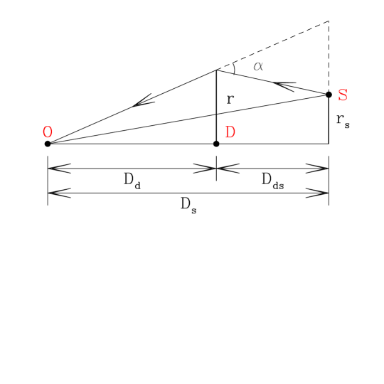
Figure 1: Basic geometry of gravitational lensing. ‘O’, ‘D’, and ‘S’ indicate the observer, deflector (lens) and source positions. $\alpha$ is the deflection angle. $r$ and $r_{\rm s}$ are the (physical) distances of the light ray and the source from the observer-lens line, respectively.

Eq. (1) can be easily solved and one finds that there are always two images for given source position, one with positive parity and one with negative parity The total magnification satisfies a simple relation (e.g., Paczyński 1986):

$$\mu=\frac{u^{2}+2}{u\sqrt{u^{2}+4}},$$ (2)

where $u=r/r_{\rm E}$. The Einstein radius $r_{\rm E}$ is given by

$$r_{\rm E}=\left({4GMD\over c^{2}}\right)^{1/2}\approx 9{\rm AU}{\left({M\over M_{\odot}}\right)}^{1/2}{\left({D\over 10{\rm kpc}}\right)}^{1/2}.$$ (3)

The angle extended by the Einstein ring on the sky is about $\sim 1$ milli-arcsecond. Notice that when $u=1$, the total magnification $\mu=3/\sqrt{5}\approx 1.342.$ Such a change of 0.32 mag can be readily detected, so the area covered by the Einstein ring is commonly used as a measure of the lensing cross section.

Since everything moves in nature, the magnification changes with time due to the change in relative alignment. So in practice we detect microlensing by the source light change. Two sample source trajectories and corresponding light curves are shown in Fig. 2. The time scale is determined by the Einstein radius crossing time

$$t_{\rm E}=78\,{\rm day}{\left({M\over M_{\odot}}\right)}^{1/2}{\left({D\over 10{\rm kpc}}\right)}^{1/2}{\left({V_{\rm t}\over 200{\rm km\,s^{-1}}}\right)}^{-1},$$ (4)

where ${V_{\rm t}}$ is the lens transverse velocity relative to the observer-source line, and $D$ is given in eq. (1). From an observed light curve, we can infer (primarily) four parameters, the baseline magnitude of the lensed object, peak magnification, peak time and the Einstein radius crossing time, $t_{\rm E}$. Since only the variable $t_{\rm E}$ carries information about the lens and since it depends on a number of parameters ($M,D_{\rm d},D_{\rm s}$ and $V_{\rm t}$), it is impossible to determine the lens mass and distance uniquely. This lens degeneracy is the most severe limitation in the current surveys and it makes a number of interpretations ambiguous (see §5). As we can see, the ‘standard’ light curves are symmetric, achromatic, and non-repeating (see eq. 5). These signatures can be used to tell microlensing from other stellar variabilities. However, there are exceptions to these rules, see Fig. 3 and §4.

So far we have concentrated on individual microlensing light curves, and we obviously need a statistical description of the lensing sample as a whole. For this purpose, two concepts come in handy: the optical depth and event rate. The optical depth is the probability that there is a lens located inside the Einstein radius at any distance along the line of sight, or equivalently, the probability that a source is magnified by more than a factor of $3/\sqrt{5}$ at any given time. For any lens number density distribution, it can be calculated as (Paczyński 1986)

$$\tau=\int_{0}^{D_{\rm s}}n~{}(\pi r_{\rm E}^{2})~{}dD_{\rm d}.$$ (5)

In particular, for a self-gravitating system with a constant rotation velocity $V$, $\tau\propto V^{2}/c^{2}$ ($\sim 5\times 10^{-7}$ for the Milky Way; the small optical depth implies that the microlensing variability is non-repetitive.) Notice that the optical depth depends only on the total mass in all lenses, but is independent of the mass function of lenses. This can be easily seen since $n\propto\rho/m$ where as $\pi r_{\rm E}^{2}\propto m$, so the product of $n$ and $\pi r_{\rm E}^{2}$ does not depend on the mass of lenses. The optical depth can therefore be used to infer the overall mass distribution of the lenses.

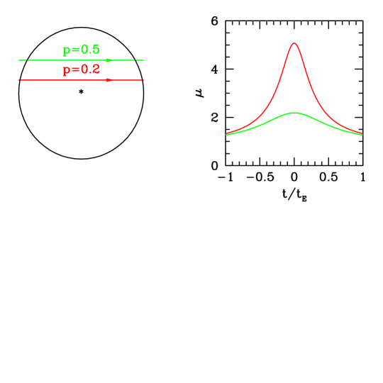
Figure 2: The left panel shows two source trajectories on the plane of sky with impact parameter (in units of $r_{\rm E}$) of $p=0.2,0.5$, respectively. The circle indicates the Einstein radius with the lens at the center. The corresponding light curves are shown in the right panel; the high amplitude one corresponds to $p=0.2$.

The event rate describes the number of events per unit time. It is related to the optical depth by (e.g., Paczyński 1986):

$$\Gamma\equiv\frac{dN_{\rm event}}{dt}=\frac{2}{\pi}~{}{N_{\star}~{}\tau}~{}\frac{1}{t_{\rm E}}~{}\epsilon(t_{\rm E}).$$ (6)

Hence, the event rate ($\Gamma$) is proportional to the number of stars monitored ($N_{\star}$) and the optical depth. It is also inversely proportional to the time-scale $t_{\rm E}$ (the shorter the events, the more we expect to see in given time interval) and modulated by the detection of efficiency as a function of $t_{\rm E}$ (nearly all microlensing surveys miss events shorter than $\la$ one day and longer than a few years). Notice that $\Gamma$ depends not only on the total mass in lenses but also on the mass function (through $t_{E}$). Hence, a detailed analysis of the event duration distribution offers a unique method to determine the lens mass function, independent of light.

4 Current Observational Status

The teams involved in primary microlensing surveys are summarized in Table 1. Most surveys are using 1-m class telescopes combined with large-format CCDs and large field-of-view (notable exceptions are the DUO campaign and part of the EROS I survey which used Schmidt plates). The last few groups listed in Table 1 are surveying M31 – some promising candidates have been published, although the contamination by variable stars (e.g., Miras) remains to be sorted out (Crotts & Tomaney 1996; Ansari et al. 1999; for information on the MEGA experiment, see Crotts 1999, this volume). These surveys use the image subtraction technique (‘pixel’ lensing) and have great potentials (see §6).

Table 1: Status of Primary Microlensing Surveys

Team	Target(s)	Events	Time	Instrument	Field of View	Colors
MACHO	Bulge	$\sim 300$	92-99	8 2Kx2K,1.3m	$42^{\prime}\times 42^{\prime}$	‘R’,‘B’
	LMC	$\sim 25$
	SMC	$\sim 2$
OGLE I	Bulge	20	92-95	2Kx2K,1m	$15^{\prime}\times 15^{\prime}$	I (+V)
OGLE II	Bulge	$\sim 150$	97-	2Kx2K,1.3m	$15^{\prime}\times 15^{\prime}$	I (+V)
	LMC	$\sim 1$
	SMC
	Sp. arms	1
EROS I	LMC	$\la 2$	91-95	CCD+Schmidt		‘R’,‘B’
EROS II	Bulge	$\sim 4$	96-	16 2Kx2K,1m	$0.7^{\circ}\times 1.4^{\circ}$	‘R’,‘B’
	LMC	1
	SMC
	Sp. arms	3
DUO	Bulge	13	94-94	1m Schmidt		$B_{J}$,R
MOA	B, L, S		95-	0.6m CCDs
AGAPE	M31	2	94-	1Kx1K,2m	$4^{\prime}\times 4.5^{\prime}$	R, B
Col/VATT	M31	$\sim 6$	94-98	CCD, 1m-4m	$\sim 15^{\prime}\times 15^{\prime}$	R, I
MEGA	M31
Munich	M31		97-	1Kx1K, 0.8m	$9^{\prime}\times 9^{\prime}$	R, I

As can be seen from Table 1, $\sim 500$ hundred events have been observed and the number is still increasing day by day. The majority of these events are discovered toward the Galactic bulge, while about $\sim 30$ events have been seen toward LMC and SMC and a few toward spiral arms (Mao 1999; R. Ansari 1999, this volume). Perhaps about $90\%$ of these events follow standard light curves; one example is shown in the left panel of Fig. 3. The remaining fraction shows deviations and are often called “exotic” events. (It is, however, unclear at the present stage whether the procedures used to select standard events are biased against these exotic events.) The so-called parallax events exhibit deviations induced by the Earth motion around the Sun (Refsdal 1966; Gould 1992); they preferentially occur in long events where the Earth moves a substantial distance around the Sun. A few such events have been reported (Alcock et al. 1995; Mao 1999). There are also light curves that are significantly modified by the finite size of the lensed stars (Gould 1994; Witt & Mao 1994; Nemiroff & Wickramasinghe 1994); $\sim 2$ such events have been reported (Alcock et al. 1997b). The most dramatic deviation occurs when the lens is a binary (e.g., Mao & Paczyński 1991). In some cases, the light curves can show multiple peaks with sharp rises and falls. One example is shown in the right panel of Fig. 3, taken from Rhie (1999; see also Afonso et al. 1999). About 30 such binary microlensing events have been seen (e.g., Udalski et al. 1994b; Alcock et al. 1999d). There are also other deviations, such as those due to binary sources (Griest & Hu 1993) and wide binaries (Di Stefano & Mao 1996). All these deviations have been predicted and later seen in the experiments. The importance of these exotic events is that they provide additional constraints on the lensing configuration. For example, the finite source size event and the binary caustic crossing events can be used to determine the transverse velocity (e.g., for 98-SMC-1, Afonso et al. 1999) while the parallax events provide a measure of the Einstein radius projected on the observer plane (in units of AU).

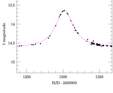
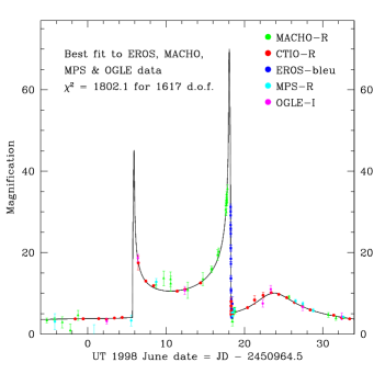
Figure 3: Examples of microlensing light curves. The left panel shows a microlensing light curve toward the Galactic bulge discovered by the OGLE collaboration in real-time; most events follow the symmetric, achromatic shape as the one shown here. The right panel shows a binary microlensing events observed by many groups (cf. Afonso et al. 1999).

5 Scientific Highlights

In this section, I highlight some of the scientific returns from the surveys. Notice that the published microlensing results are still largely based on $\sim 50$ events toward the bulge and $\sim 10$ events toward LMC.

5.1 Dark Matter

5.1.1 Planetary Mass

From eq. (6), we see that the number of events scales with the lens mass as $\propto M^{-1/2}$. Thus if the halo is dominated by low mass objects, we would expect many short duration events. Both the EROS and MACHO collaborations have searched for such short events toward LMC, none was found. A joint analysis by these collaborations (shown in Fig. 4) rules out a halo dominated by objects in the mass range of $10^{-7}M_{\odot}<M\la 10^{-2}M_{\odot}$ (Alcock et al. 1998).

Figure 4: Limits on the planetary dark matter objects in the Galactic halo. Shown here are the 95% confidence contours in the plane of the lens mass and the fraction of mass in such lenses. The various lines are for different halo models with different halo flattening and rotation curves (adapted from Alcock et al. 1998).

5.1.2 Dark matter with $M\sim M_{\odot}$

The MACHO collaboration has analyzed $\sim 8$ microlensing events toward LMC from their first two year experiment. They concluded that the optical depth is $\tau\approx 2.9^{+1.4}_{-0.9}\times 10^{-7}$ and from the even durations they estimate that the most likely lens mass is $M\sim 0.5M_{\odot}$. Since a halo full of compact objects would have $\tau\approx 5\times 10^{-7}$, their result implies that the fraction of mass in MACHOs is $\sim 50\%$. Fig. 5 shows graphically these results from a likelihood analysis (Alcock et al. 1997a).

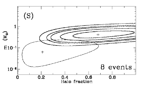
Figure 5: Limits on the dark matter objects in the Galactic halo. Shown here is the likelihood contours in the plane of the lens mass and the fraction of mass in such lenses. The contour levels are respectively 34%, 68%, 90%, 95%, and 99%. The lower left contour is the 90% limit from the first year data (adapted from Alcock et al. 1997b).

To understand this important result, we have to recall the optical depths contributed by known populations. Galactic disk populations contribute about $\tau\sim 1.5\times 10^{-8}$ (cf. Table 10 in Alcock et al. 1997b). The simplest estimates of $\tau$ for self-lensing of LMC stars by LMC stars are $\tau\approx 0.1-0.5\times 10^{-7}$ (Wu 1994; Sahu 1994). The inferred optical depth (which still has large uncertainties) is larger than these stellar contributions. So the most straightforward interpretation is that one has discovered an entirely new MACHO population. Many candidates have been proposed, such as white dwarfs, primordial black holes, dense molecular clouds etc. All these scenarios have some difficulties. For example, if the MACHOs are white dwarfs, these stars will produce too much chemical enrichment in the halo (e.g., Freese et al. 1999, and references therein). Also the high MACHO fraction is somewhat larger than the baryon fraction expected from nucleosynthesis. Nucleosynthesis predicts the density parameter in baryons $\Omega_{B}\approx 0.015h^{-2}$ (Walker et al. 1991), and hence the global baryon fraction is

$$f_{\rm B}=\frac{\Omega_{B}}{\Omega_{0}}\approx 12\%\left(\frac{H_{0}}{65{\rm\,km\,s^{-1}}}\right)^{-2}\left(\frac{\Omega_{0}}{0.3}\right)^{-1},$$ (7)

where $\Omega_{0}$ is the total matter density and $H_{0}$ is the Hubble constant. The fraction is around $\sim 10\%$ for $\Omega_{0}=0.3$, while for $\Omega_{0}=1$, the fraction is only around 4%. So there seems to be some contradictions.

In light of these difficulties, people have put forward revised scenarios of self-lensing, such as self-lensing of tidal LMC disk or lensing due to intervening stellar populations along the line of sight (Zhao 1998). The three binary microlensing events toward LMC and SMC are consistent with self-lensing. It remains controversial whether the stellar population studies support this scenario (see Zhao 1999, and references therein). It is desirable to to test different scenarios empirically. One important possibility is to use exotic microlensing events to obtain further constraints on the lens locations (see Evans 1999, this volume). We can also examine statistical properties of the lensed population (Stubbs 1998; Zhao 1999). For example, we can examine the optical depth across the LMC as a function of stellar density. For self-lensing, we expect $\tau\propto\rho_{*}^{2}$, while for lensing by dark matter objects, $\tau\propto\rho_{*}$. Also in the self-lensing scenario, the stars at the far-side of LMC is more likely to be lensed than those at the near-side, so the lensed sources should be systematically fainter and suffer more extinction and reddening (Zhao 1999 and references therein). Further, they may also have different kinematical behaviors. We return to some future possibilities in §6.

5.2 Galactic Bulge

5.2.1 Galactic Structure and Optical Depth

The OGLE collaboration gives an optical depth $\tau=(3.3\pm 1.2)\times 10^{-6}$ based on $\sim 10$ events (Udalski et al. 1994a), while the MACHO collaboration gives $\tau=3.9^{+1.8}_{-1.2}\times 10^{-6}$ (Alcock et al. 1997c) based on 45 events.

Earlier estimates showed that (Paczyński 1991; Griest et al. 1991): $\tau\sim 4-8\times 10^{-7}$, much smaller than the observed one. Taken into account the self-lensing (Kiraga & Paczyński 1994) and galactic bar structure (Zhao et al. 1996), $\tau$ was revised upward to $\sim 2\times 10^{-6}$. However, a more recent dynamical model of the Galaxy gives an optical depth of only $1.4\times 10^{-6}$ (Häfner et al. 1999), which seems to be too low. It is unclear whether the discrepancy is serious or not, since the observed $\tau$ is based on only $\sim 50$ events so far. Furthermore, the effect of blending on $\tau$ has not been estimated realistically. If the discrepancy remains when the larger (existing) database of events is analyzed, this signals that our dynamical understanding of the Galaxy may be incomplete.

5.2.2 Mass function

Fig. 6 shows the predicted duration distribution from Zhao et al. (1996). A Salpeter mass function ($dN/dM\propto M^{-2.35}$) matches the observed duration distribution very well, while one dominated by brown dwarfs predict too many short events and hence is ruled out. In contrast, the predicted distribution with a disk mass function derived from HST star counts (Han & Gould 1996) would predict too few short events. This is easy to understand since the disk mass function ($dN/dM\propto M^{-0.5}$) is significantly flatter than the Salpeter mass function at the low mass end. The bulge mass function determined using HST NICMOS data (Zoccali et al. 1999) may also be too flat to explain the observed distribution. The observations hint that the mass functions at different places in the Galaxy (in particular the disk and bulge) may be different. Some of the differences may be due to evolutionary effects, as evidenced in globular clusters (see Zoccali et al. 1999 and references therein).

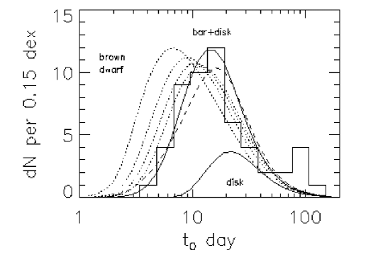
Figure 6: The histogram shows the observed distribution of event durations. The two solid lines are the predictions for the disk population and the whole population (bar+disk). The dotted lines are for different brown dwarf contributions (the leftmost one is with a 60% brown dwarf contribution). See Zhao et al. (1996) for more details.

5.3 Stellar Studies

The contribution of microlensing surveys to stellar studies is multi-fold. First, it provides excellent color-magnitude diagrams. Combined with stellar population synthesis models, they can be used to decipher different components in the Galaxy (e.g., Ng et al. 1996). Second, microlensing surveys provides tens of thousands variable stars, including cepheid variables and RR Lyrae stars. The huge database allows one, for example, to investigate the metallicity effects in cepheids, which has important implications on the cosmological distance ladder (Sasselov et al. 1997). These variable stars has also been used to infer the star formation history of the LMC (Alcock et al. 1999a). The rare detached eclipsing binaries can be used to determine the distances in a single step, to a few percent accuracy (Paczyński 1996a). The red clump stars have also been argued as a standard candle (e.g., Udalski 1998) and hence can be used to determine distances and obtain extinction maps toward the Galactic center (Stanek 1996). Highly magnified events are particularly suitable for real-time spectroscopies; a pilot program has been carried out by Lennon et al. (1996, 1997); these spectra have been used to derive the ages, abundances of the lensed stars. Interested readers are referred to the recent conference held in Budapest for more information at http://www.konkoly.hu:80/iau176/.

5.4 Planet Detection

Planet detection has become an important application of microlensing. The method was proposed a number of years ago (Mao & Paczyński 1991; Gould & Loeb 1992; Bennett & Rhie 1996; Di Stefano & Scalzo 1999). This field is maturing due to the efforts by the PLANET, MPS and other collaborations. There has been even a claim that a Jovian planet was discovered in a binary star system (Bennett et al. 1999). More complete references and discussions can be found in the review by P. Sackett (this volume).

6 Future Directions

As discussed in §5, Microlensing surveys have been very successful, producing exciting results on many branches of astronomy. However, the current surveys also have limitations. First, only $\sim 30$ events have been discovered so far toward LMC and SMC ($\sim 10$ analyzed so far!), so the results are still dominated by small number statistics. The lines of sight probed are still largely limited to the bulge, LMC, SMC and M31. Most frustratingly, due to the lens degeneracy, the lens mass, distance and hence the interpretations remain uncertain.

The future directions of microlensing research are to overcome these weaknesses in the next few years. First, there is still a large un-analyzed database, particularly toward the bulge. Analyses of these events will map the optical depth as a function of latitude and longitude and hence probe the structure of the galaxy. The distribution of event durations also places unique constraints on the mass function of stars when hundreds of microlensing are available (Mao & Paczyński 1996). For example, from microlensing toward LMC, SMC and the Galactic bulge it will be possible eventually to study the metallicity dependence of the (initial) mass functions. The second promising direction is the large-scale application of the image subtraction method (Tomaney & Crotts 1996; Alard & Lupton 1998; Alcock et al. 1999b,c). The main difficulty is to take into account the point-spread-function variations. Apparently this difficulty can be overcome, particularly with the non-constant kernel smoothing (Alard 1999). The method seems to provide more precise photometries, as a result, the event number is increased by a factor of $\sim 2$ toward the bulge. So far this method has been applied to limited data set, wider applications of this method will be an important advance on the software level. Thirdly, although the MACHO collaboration will end in 1999, the EROS II and OGLE II experiments will continue their observations. The OGLE II experiment plans to install a larger camera. This will allow the detection of a larger number of microlensing events. Another proposed experiment (Stubbs 1998) will increase the number of events toward LMC by orders of magnitude. This will put the microlensing results toward LMC on a sound statistical footing. Fourthly, the Space Interferometry Mission (to be launched in 2005), with astrometric accuracy of $\sim$ few micro-arcsecond, will in principle allow one to determine lens mass and distance uniquely for a number of events, and hence removing the lens degeneracy (e.g., Paczyński 1998; Boden, Shao & Van Buren 1998). For the followup studies, continued efforts to detect planets using microlensing should be very fruitful. Also a more systematic spectroscopic survey on 8-10m class telescopes will yield reliable ages and chemical abundances for dwarfs in the bulge; such information will be important for understanding the formation and evolution of the Galaxy.

- [1] fonso, C. et al., 1999, astro-ph/9907247
- [2] lard, C. 1999, astro-ph/9903111
- [3] lard, C., & Lupton, R. H. 1998, ApJ, 503, 325
- [4] lcock, C. et al. 1993, Nature, 365, 621
- [5] lcock, C. et al. 1995, ApJ, 454, L125
- [6] lcock, C. et al. 1996, ApJ, 463, L67
- [7] lcock, C. et al. 1997a, ApJ, 486, 697
- [8] lcock, C. et al. 1997b, ApJ, 491, 436
- [9] lcock, C. et al. 1997c, ApJ, 479, 119; erratum, 1998, ApJ, 500, 522
- [10] lcock, C. et al. 1998, ApJ, 499, L9
- [11] lcock, C. et al. 1999a, AJ, 117, 920
- [12] lcock, C. et al. 1999b, astro-ph/9903215
- [13] lcock, C. et al. 1999c, astro-ph/9903219
- [14] lcock, C. et al. 1999d, astro-ph/9907369
- [15] nsari, R. et al. 1999, A&A, 344, L49
- [16] ubourg, E. et al. 1993, Nature, 365, 623
- [17] ennett, D., & Rhie, S. H. 1996, ApJ, 472, 660
- [18] ennett, D. et al. 1999, astro-ph/9908038
- [19] oden, A. F., Shao, M., & Van Buren, D. 1998, ApJ, 502, 538
- [20] rotts, A. R. P., & Tomaney, A. B. 1996, ApJ, 473, L87
- [21] i Stefano, R., & Scalzo, R.A. 1999, ApJ, 512, 579
- [22] i Stefano, R., & Mao, S. 1996, ApJ, 457, 93
- [23] instein, A. 1936, Science, 84, 506
- [24] reese, K., Fields, B., & Graff, D. 1999, astro-ph/9904401
- [25] ould, A. 1992, ApJ, 392, 442
- [26] ould, A., & Loeb, A. 1992, ApJ, 396, 104
- [27] ould, A. 1994, ApJ, 421, L71
- [28] ould, A. 1996, PASP, 108, 465
- [29] riest, K. 1991, ApJ, 366, 412
- [30] riest, K. et al. 1991, ApJ, 372, L79
- [31] riest, K., & Hu, W. 1993, ApJ, 407, 440
- [32] an, C., & Gould, A. 1996, ApJ, 467, 540
- [33] äfner, R. M. et al. 1999, astro-ph/9905086
- [34] iebes Jr., S. 1964, Phys. Rev. 133, B835
- [35] iraga, M., & Paczyński, B. 1994, 430, L101
- [36] ennon, D. J., Mao, S., Fuhrmann, K., & Gehren, T. 1996, ApJ, 471, L23
- [37] ennon, D. J. et al. 1997, the Messenger, 90, 30
- [38] ao, S. 1999, astro-ph/9909197
- [39] ao, S., & Paczyński, B. 1991, ApJ, 374, L37
- [40] ao, S., & Paczyński, B. 1996, ApJ, 473, 57
- [41] emiroff, R.J., & Wickramasinghe, W.A.D.T., 1994, ApJ, 424, L21
- [42] g, Y. K., Bertelli, G., Chiosi, C., Bressan, A. 1996, A&A, 310, 771
- [43] aczyński, B. 1986, ApJ, 304, 1
- [44] aczyński, B. 1991, ApJ, 371, L63
- [45] aczyński, B. 1996a, in IAU symposium 173, 199
- [46] aczyński, B. 1996b, ARA&A, 34, 419
- [47] aczyński, B. 1998, ApJ, 494, L23
- [48] efsdal, S. 1964, MNRAS, 128, 295
- [49] efsdal, S. 1966, MNRAS, 134, 315
- [50] hie, S. 1999, astro-ph/9903024
- [51] oulet, E., & Mollerach, S. 1997, Phys. Reports, 279, 67
- [52] asselov, D. D. et al. 1997, A&A, 324, 471
- [53] ahu, K. C. 1994, Nature, 370, 275
- [54] tanek, Z. Z. 1996, ApJ, 460, L37
- [55] pergel, D. N. S. 1997, in Unsolved Problems In Astrophysics, Princeton University Press: Princeton, 221
- [56] tubbs, C. 1998, astro-ph/9810488
- [57] omaney, A. B., & Crotts, A. P. S. 1996, AJ, 112, 2872
- [58] dalski, A. et al. 1993, Acta Astron., 43, 289
- [59] dalski, A., Szymanski, M., Kaluzny, J. et al. 1994a, Acta Astron., 44, 227
- [60] dalski, A. et al. 1994b, ApJ, 436, L103
- [61] dalski, A. et al. 1998, Acta Astronomica, 48, 383
- [62] alker, T. P. et al. 1991, ApJ, 376, 51
- [63] itt, H. J., & Mao, S. 1994, ApJ, 430, 505
- [64] u, X. P. 1994, ApJ, 435, 66
- [65] hao, H. S., Rich, R. M., & Spergel, D. 1996, MNRAS, 278, 488
- [66] hao, H. S. 1998, MNRAS, 294, 139
- [67] hao, H. S. 1999, astro-ph/9902179
- [68] occali, M. et al. 1999, astro-ph/9906452