Semi-Analytical Models for the Formation of Disk Galaxies:
I. Constraints from the Tully-Fisher Relation

Abstract

We present new semi-analytical models for the formation of disk galaxies with the purpose of investigating the origin of the near-infrared Tully-Fisher (TF) relation. The models assume that disks are formed by cooling of the baryons inside dark halos with realistic density profiles, and that the baryons conserve their specific angular momentum. Adiabatic contraction of the dark halo is taken into account, as well as a recipe for bulge formation based on a self-regulating mechanism that ensures disks to be stable. Only gas with densities above the critical density given by Toomre’s stability criterion is considered eligible for star formation. A Schmidt law is assumed to prescribe the rate at which this gas is transformed into stars. The introduction of the star formation threshold density proves an essential ingredient of our models, and yields gas mass fractions that are in excellent agreement with observations. Finally, a simple recipe for supernovae feedback is included. We emphasize the importance of extracting the proper luminosity and velocity measures from the models, something that has often been ignored in the past. We use the zero-point of the $K$-band TF relation to place stringent constraints on cosmological parameters. In particular, we rule out a standard cold dark matter universe, in which disk galaxies are too faint to be consistent with observations. The TF zero-point, in combination with nucleosynthesis constraints on the baryon density, and with constraints on the normalization of the power spectrum, requires a matter density $\Omega_{0}\lesssim 0.3$. The observed $K$-band TF relation has a slope that is steeper than simple predictions based on dynamical arguments suggest. Taking the stability related star formation threshold densities into account steepens the TF relation and decreases its scatter. However, in order for the slope to be as steep as observed, further physics are required. We argue that the characteristics of the observed near-infrared TF relation do not reflect systematic variations in stellar populations, or cosmological initial conditions. In fact, feedback seems an essential ingredient in order to explain the observed slope of the $K$-band TF relation. Finally we show that our models provide a natural explanation for the small amount of scatter that makes the TF relation useful as a cosmological distance indicator.

1. Introduction

Within the standard picture for galaxy formation, in which galaxies are thought to form out of the gas which dissipatively collapses within the potential wells provided by virialized dark halos (White & Rees 1978), disk galaxies take a special place. Their flatness and rotational support suggest a relatively smooth formation history without violent non-linear processes. The structure and dynamics of disk galaxies are thus expected to be strongly related to the properties of the dark halos in which they are embedded. This principle is in fact the key idea behind the standard model for disk formation which was set out by Fall & Efstathiou (1980), and which has since been extended upon by numerous investigators (Faber 1982; Fall 1983; van der Kruit 1987; Dalcanton, Spergel & Summers 1997; Mo, Mao & White 1998; van den Bosch 1998). In this picture, the gas radiates its binding energy but retains its angular momentum, thus settling into a rotationally supported disk, the scale length of which is proportional to both the size and the angular momentum of the dark halo.

Understanding galaxy formation is intimately linked to understanding the origin of the fundamental scaling relations of galaxies. In this paper we use new semi-analytical models for the formation of disk galaxies to investigate the origin of the Tully-Fisher (hereafter TF) relation (Tully & Fisher 1977), which has the form

$$L=A\,V_{\rm rot}^{\gamma},$$ (1)

or, in terms of a linear law in a log-log plane:

$$M=a+b\,{\rm log}V_{\rm rot},$$ (2)

where $M$ is the absolute magnitude of the disk, and $b=-2.5\gamma$ is called the slope of the relation. In the light of the strong coupling between disk and dark halo mentioned above, a scaling relation like this is central to theories of galaxy formation. Understanding its origin can put constraints on theories of galaxy formation, and in particular on the detailed physics that cause the baryonic component of a dark halo to be transformed into a luminous galaxy. As such, any successful theory of (disk) galaxy formation should be able to explain the slope, zero-point, and small amount of scatter of this fundamental scaling relation.

Numerous studies in the past have addressed the origin of the TF relation. However, no consensus has been reached, and it is currently still under debate whether the origin of the TF relation is mainly governed by initial cosmological conditions (e.g., Eisenstein & Loeb 1996; Avila-Reese, Firmani & Hernández 1998; Firmani & Avila-Reese 1998a,b), or by the detailed processes governing star formation (Silk 1997; Heavens & Jiminez 1999) and/or feedback (e.g., Kauffmann, White & Guiderdoni 1993; Cole et al. 1994; Elizondo et al. 1999; Natarajan 1999).

One of the main reasons for this lack of consistency is the discordant use of luminosity and rotation measures in TF relations. The slope and scatter of the TF relation depend strongly on the photometric band used to measure the luminosities: values of $\gamma$ increase from $\sim 2.5$ in the $B$-band to $\sim 4$ in the infrared (e.g., Aaronson, Huchra & Mould 1979; Visvanathan 1981; Tully, Mould & Aaronson 1982; Wyse 1982; Pierce & Tully 1988; Gavazzi 1993; Verheijen 1997). For the rotation velocity a large number of different measures have been used: HI line widths from single-dish observations, velocities measured from H$\alpha$ rotation curves, rotation velocities at a fixed number of disk scale lengths, maximum observed rotation velocities, rotation velocities at the last measured point, and the velocity of the flat part of the rotation curve. All these different measures yield wildly different TF relations (see Courteau 1997 and Verheijen 1997 for detailed discussions). Therefore it is crucial that one extracts the same quantities from the models as the ones used in the empirical relation whose origin one seeks to explain. Most previous studies have ignored the subtleties associated with these different measures, and allowed themselves the “freedom” to compare their model predictions with the best fitting TF relation available in the literature.

The other reason why we still lack consensus on the origin of the TF relation regards the modeling techniques that have been used. Several investigators have used numerical simulations (e.g., Evrard, Summers & Davis 1994; Navarro & White 1994; Steinmetz & Müller 1994; Tissera, Lambas & Abadi 1997; Domínguez-Tenreiro, Tissera & Sáiz 1998; Steinmetz & Navarro 1999; Elizondo et al. 1999). A general problem, however, is that the disks that form in these simulations have specific angular momenta that are more than an order of magnitude lower than those of observed disks. In addition, most of these simulations ignore star formation and feedback, making a direct comparison between simulated and observed disks a treacherous enterprise (see Evrard 1997 for a review). Semi-analytical modeling (SAM) of galaxy formation has been more successful (White & Frenk 1991; Cole 1991; Kauffmann, White & Guiderdoni 1993; Lacey et al. 1993; Cole et al. 1994; Heyl et al. 1995; Somerville & Primack 1998). Despite reasonable success in reproducing certain TF relations, these models are hampered by several shortcomings (see discussion in § 3). More recently, Avila-Reese, Firmani & Hernández (1998; hereafter AFH98) and Firmani & Avila-Reese (1998a,b; hereafter FA98) presented new SAMs that focus only on the formation of disk galaxies. These models improve upon previous SAMs in several important ways. From a detailed comparison with observed TF relations, these authors conclude that the TF relation represents a fossil of the primordial density fluctuation field.

In this paper we present new semi-analytical models for the formation of disk galaxies. We improve upon previous studies by (i) making a well-motivated choice for the luminosity and velocity measures that define the TF relation whose origin we seek to understand, (ii) by extracting the same measures from the models, and (iii) by using new semi-analytical models that focus on the formation of disk galaxies and that alleviate several shortcomings of previous models. The main aim of this paper is to investigate the prevailing mechanism that is responsible for the slope, zero-point and small amount of scatter of the TF relation. Although our models are, in many ways, complementary to those of FA98, we reach a different conclusion.

2. The Empirical Tully-Fisher Relation

One of the most detailed investigations of the empirical TF relation is that of Verheijen (1997, hereafter V97), who obtained $B$, $R$, $I$, and $K$ band photometry, as well as detailed HI synthesis observations of a complete sample of (bright) spiral galaxies in the Ursa Major cluster (see also Tully et al. 1996). V97 made a detailed comparison of different TF relations using different photometric bands and different velocity measures. This study has yielded a number of important results: (i) the scatter in the TF relation is smallest when using the flat part of the HI rotation curve, $V_{\rm flat}$, as velocity measure, (ii) when using the HI line widths, the TF relations become shallower and harbor a larger scatter, (iii) the results of Sprayberry et al. (1995) and Zwaan et al. (1995), that high surface brightness (HSB) and low surface brightness (LSB) spirals follow the same TF relation, are confirmed, (iv) both the scatter and the slope of the TF relation are extremely sensitive to selection criteria, and (v) the slope of the TF relation changes from $b=-6.7$ in the $B$-band to $-10.5$ in the $K$-band.

Luminosities depend more strongly on extinction, stellar populations, star formation histories, and metallicities going towards bluer passbands. Given the large uncertainties associated with stellar population models and with a proper treatment of extinction by dust, and since the TF relation is fundamentally a dynamical law, the most natural passbands to use are those in the near-infrared in which luminosity is most directly related to the luminous mass (see e.g., Gavazzi 1993; Gavazzi, Pierini & Boselli 1996). If we further limit ourselves to TF relations that are not based on HI line widths, since these are particularly hard to interpret in terms of fundamental parameters of the galaxy (e.g., Haynes et al. 1999), the available data becomes actually very limited. The only TF relation that is based on full near-infrared imaging (rather than aperture photometry) and has velocity measures that are derived from full HI rotation curves, is the $K$-band TF relation of V97:

$$M_{K}-5\,{\rm log}h=0.683-10.5\,{\rm log}V_{\rm flat},$$ (3)

Here $V_{\rm flat}$ is the measured rotation velocity at the flat part of the HI rotation curve and $h=H_{0}/(100\>{\rm km}\,{\rm s}^{-1}{\rm Mpc}^{-1})$. Magnitudes have been converted to $M_{K}-5\,{\rm log}h$ adopting a distance to the Ursa Major cluster of 15.5 Mpc, which corresponds to $H_{0}=85\>{\rm km}\,{\rm s}^{-1}\,{\rm Mpc}^{-1}$ (Pierce & Tully 1988, 1992). In what follows we consider equation (3) the ‘fundamental’ TF relation whose origin we seek to understand.

3. Modeling the Formation of Disk Galaxies

In order to investigate whether the origin of the TF relation is mainly related to cosmological initial conditions, or to details regarding the processes associated with star formation and/or supernovae feedback, we construct new semi-analytical models that focus on the near-infrared properties of disk galaxies only. We incorporate a number of improvements over previous SAMs, all of which (except for FA98) assumed all dark halos to have the same specific angular momentum. Since the angular momentum sets, to a large degree, the surface density of the disk, and since star formation is a strong function of surface density (see § 3.3), a realistic spread in halo specific angular momenta yields a spread in luminosities for galaxies forming in halos of the same mass. This is especially important when investigating for example the scatter in the TF relation. Also, we take adiabatic contraction into account (Blumenthal et al. 1986; Flores et al. 1993) and consider the more realistic universal halo density profiles, rather than singular isothermal spheres, which have been found to poorly fit the actual density profiles of dark halos in $N$-body simulations (e.g., Frenk et al. 1988; Efstathiou et al. 1988; Dubinski & Carlberg 1991; Navarro, Frenk & White 1995, 1996, 1997; Tormen, Bouchet & White 1997). We use a star formation recipe that is different from previous SAMs, and mimic observations of the actual rotation curve of the galaxy, rather than to simply assume that the observed rotation velocity is equal to the circular velocity at the halo’s virial radius. As we show below, these latter two modifications prove to be of crucial importance.

The dynamical fragility of disks implies that their mass aggregation histories can not have been too violent (e.g., Tóth & Ostriker 1992). We therefore refrain from calculating complete merger histories of the dark halos. The study by Navarro et al. (1997) has shown that virialized dark halos are well described by a universal density profile, whose properties can be calculated from the Press-Schechter formalism. In a recent study, Jing (1999) has shown that halos with significant amounts of substructure can deviate significantly from this universal density profile. However, these halos are unlikely to yield disk galaxies, and the universal density profiles can thus be used to describe the end-state of the mass aggregation histories of halos surrounding spiral galaxies (see also AFH98).

As shown by Baugh, Cole & Frenk (1996), the merging histories and star formation histories are well coupled. Ignoring (small) mergers therefore mainly reflects on the details regarding the star formation histories. Since we focus on the near-infrared properties, we are insensitive to such details, given the fact that mass-to-light ratios in the near-infrared depend only very weakly on age and/or metallicity (see § 3.5 below). Furthermore, the quiet mass aggregation histories of disk galaxies implies smooth star formation histories with little scatter (Baugh et al. 1996). Therefore, in the SAMs presented here we do not follow the detailed time-resolved formation of disk galaxies, but limit ourselves to modeling the time-integrated properties.

3.1. Properties of the dark matter halos

Virialized dark halos can be quantified by a mass, $M_{200}$, a radius, $r_{200}$, and an angular momentum, $J$, originating from cosmological torques (e.g., Hoyle 1953). Here $r_{200}$ is defined as the radius inside of which the average density of the system is 200 times the critical density of the Universe, and $M_{200}$ is simply the total mass inside $r_{200}$. In a series of papers Navarro, Frenk & White (1995, 1996, 1997) showed that virialized dark halos have universal equilibrium density profiles, independent of mass or cosmology, which can be well fit by

$$\rho(r)=\rho_{\rm crit}{\delta_{0}\over(r/r_{s})(1+r/r_{s})^{2}},$$ (4)

where

$$\delta_{0}={200\over 3}{c^{3}\over{\rm ln}(1+c)-c/(1+c)},$$ (5)

with $c=r_{200}/r_{s}$ the concentration parameter, and $r_{s}$ a scale radius. Given the mass $M_{200}$ and the specific cosmology, the concentration parameter $c$ can be calculated using the procedure outlined in the Appendix of Navarro et al. (1997). In what follows we only consider spherical halos, and we refer to halos with the density profile of equation (4) as NFW halos.

The angular momentum of the halo is quantified by the dimensionless spin parameter, $\lambda$, defined by

$$\lambda={J|E|^{1/2}\over GM_{200}^{5/2}}.$$ (6)

Here $E$ is the halo’s total energy. Several studies, both analytical and numerical, have shown that the distribution of spin angular momenta of collapsed dark matter halos is well approximated by a log-normal distribution:

$$p(\lambda){\rm d}\lambda={1\over\sigma_{\lambda}\sqrt{2\pi}}\exp\biggl{(}-{{\rm ln}^{2}(\lambda/\bar{\lambda})\over 2\sigma^{2}_{\lambda}}\biggr{)}{{\rm d}\lambda\over\lambda},$$ (7)

(e.g., Barnes & Efstathiou 1987; Ryden 1988; Cole & Lacey 1996; Warren et al. 1992). We consider a distribution that peaks around $\bar{\lambda}=0.05$ with $\sigma_{\lambda}=0.6$. These values are in good agreement with the $N$-body results of Warren et al. (1992), and virtually independent of cosmology (e.g., Lemson & Kauffmann 1999).

3.2. The formation of disk and bulge

Once the halo properties are known, we can determine the global properties of the disks that form inside them. The virialization of the halo heats the baryonic matter to the virial temperature. As the baryons start to cool they loose their pressure support and settle in a disk. We follow Fall & Efstathiou (1980) and assume that the specific angular momentum of the baryonic material is conserved. We further assume that the disk that forms has an exponential surface density profile. The scale-length of the disk is proportional to $\lambda$ and $r_{200}$, and can be calculated using equation (28) in Mo et al. (1998).

Self-gravitating disks tend to be unstable against global instabilities such as bar formation. We use the stability criterion of Christodoulou, Shlosman & Tohline (1995), according to which disks are stable if they obey

$$\alpha={V_{d}\over 2V_{c}}<\alpha_{\rm crit},$$ (8)

with $V_{d}$ and $V_{c}$ the characteristic circular velocities of the disk and the composite disk-bulge-halo system, respectively . As characteristic velocities we consider the circular velocities at $R=3R_{d}$, since Mo et al. (1998) have shown that this is the radius where typically the rotation curve of the composite system reaches a maximum. We set $\alpha_{\rm crit}=0.35$ throughout, as suggested for gaseous disks (Christodoulou et al. 1995). We have tested that none of our results depend significantly on the value of this parameter.

We follow the approach of van den Bosch (1998, 1999) and assume that a gaseous disk which is unstable according to criterion (8) transforms part of its disk material into a bulge component in a self-regulating fashion, such that the final disk is marginally stable (i.e., $\alpha=\alpha_{\rm crit}$). We describe the bulge by a sphere with a Hernquist density profile:

$$\rho_{b}(r)={M_{b}\over 2\pi}\,{r_{b}\over r\,(r+r_{b})^{3}},$$ (9)

where $r_{b}$ is a scale length (Hernquist 1990). Andredakis, Peletier & Balcells (1995) have shown that the effective radius $r_{e}$ (defined as the radius encircling half of the projected light) is directly related to the total luminosity of the bulge by the empirical relation

$$M_{B}=-19.75-2.8\,{\rm log}(r_{e})$$ (10)

If we now use $M_{B}-M_{K}=4.0$, in good agreement with the average value for bulges (Peletier & Balcells 1997), and $r_{e}=1.8153\,r_{b}$ (Hernquist 1990), we obtain

$$r_{b}=0.71\,\left({L_{b,K}\over 10^{11}\>{\rm L_{\odot}}}\right)^{0.89}\,{\rm kpc},$$ (11)

which we use to set the scale length of the bulges in our models. Our results do not depend on this simple scaling assumption, in practice. The main parameter for the bulge is its total mass; changes in its actual density distribution are only a second-order effect, and do not influence our results.

3.3. Star formation

Since the $K$-band mass-to-light ratio depends only weakly on the metallicity and age of a stellar population (see § 3.5), and since integrated star formation histories of disk galaxies are not expected to exhibit strong variety, the main parameter of interest is the fraction of the gas that is converted into stars over the lifetime of the galaxy.

In a seminal paper Kennicutt (1989) showed that star formation is abruptly suppressed below a critical surface density, which is associated with the onset of large-scale gravitational instabilities, and which can be modeled by a simple Toomre disc stability criterion:

$$\Sigma_{\rm crit}(R)={\sigma_{\rm gas}\,\kappa(R)\over 3.36\,G\,Q}$$ (12)

(Toomre 1964). Here $Q$ is a dimensionless constant near unity, $\sigma_{\rm gas}$ is the velocity dispersion of the gas, and $\kappa$ is the epicycle frequency given by

$$\kappa(R)=\sqrt{2}\;{V_{c}(R)\over R}\left(1+{R\over V_{c}(R)}{{\rm d}V_{c}\over{\rm d}R}\right)^{1/2}.$$ (13)

This critical density sets the fraction of the gas that is eligible for star formation (see also Quirk 1972). Given the exponential surface density of the gas disk, with scale length $R_{d}$ and central surface density $\Sigma_{0}$, the radius $R_{\rm SF}$, at which the density of the disk equals $\Sigma_{\rm crit}$ can be calculated. The disk mass inside this radius, and with surface density above $\Sigma_{\rm crit}$ is considered eligible for star formation (cf. Quirk 1972; Kauffmann 1996). Unless stated otherwise we adopt $\sigma_{\rm gas}=6\>{\rm km}\,{\rm s}^{-1}$ and $Q=1.5$, as these values have been shown by Kennicutt (1989) to yield values of $R_{\rm SF}$ that correspond to the radii at which star formation is truncated.

What remains is to quantify the fraction, $f_{\rm SF}$, of this eligible mass that is actually turned into stars over the age of the galaxy. The star formation rate of disk galaxies is well fitted by a simple Schmidt (1959) law:

$$\psi_{\rm SFR}=a\,\Sigma^{n}_{\rm gas}$$ (14)

For a large sample of disk galaxies, Kennicutt (1998) found $a=0.25\pm 0.07\>{\rm M_{\odot}}{\rm pc}^{-2}{\rm Gyr}^{-1}$ and $n=1.4\pm 0.15$. If we assume that a fraction $\epsilon_{\rm SF}$ of the mass formed in new stars is (instantaneously) returned to the gas phase by means of stellar winds and supernovae, one obtains for the gas density at the present

$$\Sigma_{\rm gas}(R)=\left[-{A_{\rm SF}\over m}t_{\rm gal}+\left(\Sigma_{0}{\rm e}^{-R/R_{d}}\right)^{1/m}\right]^{m}$$ (15)

(cf. Heavens & Jiminez 1999), with $m=1/(1-n)$, $A_{\rm SF}=(1-\epsilon_{\rm SF})\,a$, and $t_{\rm gal}$ the age of the galaxy, which we define as the time since the halo’s collapse. If we now couple this to the threshold density criterion, we can calculate the total mass in stars formed in the disk. If we further assume that all the gas that is transformed into a bulge component forms stars at 100 percent efficiency, we obtain

$$M_{*}=M_{b}+2\pi\int\limits_{0}^{R_{\rm SF}}\left[\Sigma_{0}{\rm e}^{-R/R_{d}}-g(R)\right]R\,{\rm d}R$$ (16)

with

$$g(R)=\left\{\begin{array}[]{ll}\Sigma_{\rm gas}(R)&\mbox{$\;\;\;\;\;(\Sigma_{\rm gas}>\Sigma_{\rm crit})$}\\ \Sigma_{\rm crit}(R)&\mbox{$\;\;\;\;\;(\Sigma_{\rm gas}\leq\Sigma_{\rm crit})$}\end{array}\right.$$ (17)

Thus, the surface density of the gas is not allowed to drop below the critical density given by equation (12).

The total $K$-band luminosity of the disk-bulge system then follows from $L_{K}=M_{*}/\Upsilon^{*}_{K}$, where $\Upsilon^{*}_{K}$ is the mass-to-light ratio of the stellar mass.

3.4. Feedback from supernovae

The dominant source of feedback that can keep gas out of the disk is provided by supernovae (SN). A mass $M_{*}$ of stars produces a total amount of energy by SN equal to

$$E_{\rm total}=\eta_{\rm SN}\,M_{*}\,E_{\rm SN}$$ (18)

Here $E_{\rm SN}$ is the energy produced by one SN, and $\eta_{\rm SN}$ is the number of SN expected per solar mass of stars formed. Throughout we adopt $\eta_{\rm SN}=4\times 10^{-3}\>{\rm M_{\odot}}^{-1}$, consistent with a Scalo (1986) initial mass function (IMF).

In what follows, we assume that this amount of energy can prevent a mass $M_{\rm hot}$ from ending up in the final disk-bulge system, either by means of completely expelling the gas from the halo, or by keeping gas in the halo at the virial temperature, thus preventing its collapse to the disk. Taking account of the escape velocity of the halo, and requiring energy balance, one obtains

$$M_{\rm hot}={M_{*}\,\varepsilon_{\rm SN}\,\eta_{\rm SN}\,E_{\rm SN}\over V_{200}^{2}}$$ (19)

(cf. Kauffmann et al. 1993; Natarajan 1999), where we introduce a new parameter, $\varepsilon_{\rm SN}$, which is a measure of the efficiency with which the SN energy can prevent the gas from ending up in the disk or bulge. One might imagine that the free parameter $\epsilon_{\rm SN}$ is not constant for all galaxies, and we therefore introduce the following simple scaling relation

$$\varepsilon_{\rm SN}=\varepsilon_{\rm SN}^{0}\left(V_{200}\over 250\>{\rm km}\,{\rm s}^{-1}\right)^{\nu},$$ (20)

We can now define the fraction

$${M_{\rm hot}\over M_{*}}=3.22\,\varepsilon_{\rm SN}^{0}\times$$ (21)

$$\left({\eta_{\rm SN}\over 0.004\>{\rm M_{\odot}}^{-1}}\right)\left({E_{\rm SN}\over 10^{51}{\rm erg}}\right)\left({V_{200}\over 250\>{\rm km}\,{\rm s}^{-1}}\right)^{\nu-2}.$$

Thus, in a halo with $V_{200}=250\>{\rm km}\,{\rm s}^{-1}$, a mass $M_{*}$ in stars can prevent a mass $3.22\,\varepsilon_{\rm SN}^{0}\,M_{*}$ from settling in the disk or bulge. Stellar winds from evolving young stars add to the energy released by SN, and we therefore allow values of $\varepsilon_{\rm SN}$ in excess of unity.

We can now combine the star formation recipe outlined in § 3.3 with this feedback model to determine the masses in the different phases: $M_{*}$, $M_{\rm hot}$, and $M_{\rm cold}$, where the latter is the amount of (cold) gas in the disk that is not turned into stars. Mass conservation requires $M_{*}+M_{\rm cold}+M_{\rm hot}=M_{\rm baryons}$. Defining $\epsilon_{\rm gf}$ as the galaxy formation efficiency, which describes what fraction of the baryonic mass inside the halo ultimately ends up in the disk/bulge, i.e.,

$$M_{d}+M_{b}=\epsilon_{\rm gf}\,f_{\rm bar}\,M_{200},$$ (22)

we can write

$$\epsilon_{\rm gf}=\left[1+{M_{\rm hot}\over M_{d}+M_{b}}\right]^{-1}.$$ (23)

This equation can not be solved analytically, as $M_{\rm hot}$, $M_{d}$ and $M_{b}$ all depend on $\epsilon_{\rm gf}$. However, as we outline in § 3.6, we can solve for $\epsilon_{\rm gf}$ using an iterative procedure.

Since circular velocities depend on whether or not the hot gas is expelled from the halo, we introduce the parameter $f_{\rm esc}$, which describes what fraction of $M_{\rm hot}$ actually escapes the halo. The remaining fraction is assumed to be at virial temperature and to follow the same density profile as the dark matter. It is straightforward to show that

$${V_{c}(f_{\rm esc}=1)\over V_{c}(f_{\rm esc}=0)}<\sqrt{1-f_{\rm bar}}.$$ (24)

This upper limit is reached in the limit where $\epsilon_{\rm gf}\rightarrow 0$, and thus applies to very low mass systems for which the SN feedback is most efficient. For a baryon fraction of $f_{\rm bar}=0.05$, neglecting $f_{\rm esc}$ thus yields errors on the circular velocities that never exceed 3 percent. Lacking a physically well-motivated value for $f_{\rm esc}$ and given its insignificance for the results presented in this paper, we set $f_{\rm esc}=0.5$ throughout, i.e., midway its two extremes.

3.5. Stellar populations

In order to convert stellar masses to luminosities we need to adopt a mass-to-light ratio for the stellar population, $\Upsilon^{*}_{K}$. In the near-infrared the mass-to-light ratios of stellar populations are fairly independent of metallicity and age, but these dependencies increase strongly going towards bluer passbands (e.g., Maraston 1998a,b). By focusing on the near-infrared TF relation we are thus less sensitive to uncertainties related to stellar populations (or extinction by dust). Using the latest version of the Bruzual & Charlot (1993) population synthesis models, we compute the $K$-band mass-to-light ratio of a stellar population with a Scalo IMF that has been producing stars with a constant rate over the past $10$ Gyr (a typical value for the age of galaxies since collapse). We find a value of $\Upsilon^{*}_{K}=0.4$ and, unless stated otherwise, we adopt this value throughout.

3.6. Constructing a catalogue of model galaxies

We now combine all the recipes outlined above to construct a catalogue of model galaxies. After choosing a cosmology (see Table 1) and setting the free parameters in our model, we proceed as follows:

First we randomly assign the halo a mass in the range $6.3\times 10^{9}\,h^{-1}\,\>{\rm M_{\odot}}\leq M_{200}\leq 3.6\times 10^{12}\,h^{-1}\,\>{\rm M_{\odot}}$, corresponding to $30\,\>{\rm km}\,{\rm s}^{-1}\leq V_{200}\leq 250\,\>{\rm km}\,{\rm s}^{-1}$. We use the procedure outlined in the Appendix of Navarro et al. (1997) to compute the halo’s collapse redshift, $z_{\rm coll}$, from which we calculate the age $t_{\rm gal}$ and the halo concentration parameter $c$. Next we randomly draw a value for the halo’s spin parameter from the probability distribution of equation (7).

We start by assuming that all the baryons settle in a disk (i.e., $\epsilon_{\rm gf}=1$ and $M_{b}=0$). Taking adiabatic contraction into account, we compute the scale-length and central surface brightness of the disk (see Mo et al. 1998, and van den Bosch 1998 for details). Next we use equation (8) to check whether the disk is stable. If $\alpha>\alpha_{\rm crit}$, an iterative procedure is used to compute the bulge mass that yields $\alpha=\alpha_{\rm crit}$ (each iteration step, the procedure for the adiabatic contraction is repeated). After convergence, we compute $M_{*}$ and $M_{\rm hot}$, from which we obtain a new estimate for the galaxy formation efficiency, $\epsilon_{\rm gf}$. We iterate this entire procedure until $M_{*}+M_{\rm cold}+M_{\rm hot}$ is equal to the total baryonic mass, yielding a completely self-consistent disk-bulge-halo model.

Finally we extract the observational quantities that enter in the TF relation. The luminosity of the disk in the $K$-band is determined from $M_{*}$ using the mass-to-light ratio $\Upsilon^{*}_{K}$. As velocity measure, we use the rotation velocity at the last measured point of the HI rotation curve of the model galaxy. For observed galaxies, this point basically coincides with the position at which the HI column density, N[HI], falls below the detectability limit of the observations, and is typically of the order of $10^{20}{\rm cm}^{-2}$. Since this column density is a projected quantity, the radius of the last measured point depends on both the surface density of the disk, and its inclination angle with respect to the line-of-sight. We therefore draw a random inclination angle, $i_{\rm min}\leq i\leq i_{\rm max}$, and calculate the circular velocity, $V_{\rm obs}$, at the radius where the projected HI column density is equal to $10^{20}{\rm cm}^{-2}$. As mentioned in § 2, the TF relation whose origin we seek to understand (equation [3]) is based on $V_{\rm flat}$, i.e., the velocity at the flat part of the rotation curve. In Figure 1 we show that the velocity at the radius where ${\rm N[HI]}=10^{20}{\rm cm}^{-2}$ is a good representation of $V_{\rm flat}$, justifying our choice of velocity measure.

Throughout we assume that $\Sigma_{\rm gas}=1.3\Sigma_{\rm HI}$ to take account of the mass of helium. Unless stated otherwise we set $i_{\rm min}=45^{\rm o}$ and $i_{\rm max}=90^{\rm o}$ as this corresponds to the typical values that observers use to select galaxies for their TF samples. Since the TF relation of equation (3), which we use to constrain our models, is based on spirals of Hubble type Sb or later, we only allow model galaxies in our sample with bulge-to-disk ratios $B/D\leq 0.2$.

4. Cosmological constraints from the Tully-Fisher zero-point

It is straigthforward to show that simple dynamics predict a TF relation with a slope of $-7.5$ (Dalcanton et al. 1997; White 1997; Mo et al. 1998; van den Bosch 1998; Syer, Mao & Mo 1999). For the baryon density we adopt here ($\Omega_{\rm bar}=0.0125\,h^{-2}$) the predicted TF can be written as

$$L_{K}=7.73\times 10^{10}{\epsilon_{\rm gf}\over h^{3}\,\Omega_{0}}\left({\Upsilon_{K}\over 0.3}\right)^{-1}\left({V_{200}\over 200\>{\rm km}\,{\rm s}^{-1}}\right)^{3},$$ (25)

(cf. equation [28] in van den Bosch 1998). The observed $K$-band TF relation of equation (3) in power-law form reads

$$L_{K}=5.68\times 10^{10}\,h^{-2}\left({V_{\rm flat}\over 200\>{\rm km}\,{\rm s}^{-1}}\right)^{4.2}.$$ (26)

Upon equating the zero-points of the observed and predicted TF relations at $V_{200}=200\>{\rm km}\,{\rm s}^{-1}$ we obtain

$$\Omega_{0}\,h=1.363\,\epsilon_{\rm gf}\,\left({\Upsilon_{K}\over 0.3}\right)^{-1}\,\left({V_{\rm flat}\over V_{200}}\right)^{-4.2}.$$ (27)

This equation immediately suggests that by setting reasonable limits on $\epsilon_{\rm gf}$, $\Upsilon_{K}$, and $V_{\rm flat}/V_{200}$, we can place strong upper bounds on $\Omega_{0}\,h$. The mass-to-light ratio $\Upsilon_{K}$ in equations (25) and (27) is defined as the ratio of mass over $K$-band luminosity for the disk. Since not all the mass of the disk is transformed into stars, this is not equal to the stellar mass-to-light ratio $\Upsilon_{K}^{*}$, i.e.,

$$\Upsilon_{K}=\Upsilon_{K}^{*}\,{M_{d}\over M_{*}}$$ (28)

and in general $\Upsilon_{K}>\Upsilon_{K}^{*}$. Using the Bruzual & Charlot (1993) stellar population models, we find that $\Upsilon_{K}^{*}\gtrsim 0.3\>{\rm M_{\odot}}/\>{\rm L_{\odot}}$ for a Scalo IMF, at least if the $K$-band light is not dominated by a young ($\lesssim 1$ Gyr) population. The $K$-band mass-to-light ratio depends rather strongly on IMF (much more so than on age and/or metallicity). However, most other IMFs that are frequently used, such as the Salpeter IMF, have higher mass fractions at the low mass end, and therefore yield higher mass-to-light ratios. We can thus consider $\Upsilon_{K}=0.3\>{\rm M_{\odot}}/\>{\rm L_{\odot}}$ a conservative lower limit. Together with the physical constraint that $\epsilon_{\rm gf}\leq 1$, we obtain

$$\Omega_{0}\,h\leq 1.363\,\left({V_{\rm flat}\over V_{200}}\right)^{-4.2}.$$ (29)

The ratio $V_{\rm flat}/V_{200}$ depends on the concentration of the dark halo, $c$, which, for given $\Omega_{0}$, $\Omega_{\Lambda}$ and $h$, depends on the normalization of the power spectrum, $\sigma_{8}$. Higher values of $\sigma_{8}$ yield more centrally concentrated halos, giving rise to higher values of $V_{\rm flat}/V_{200}$. Equation (29) thus yields an empirical constraint on a combination of $\Omega_{0}$, $\Omega_{\Lambda}$, $h$, and $\sigma_{8}$.

The constraint of equation (29) is over-conservative, in that all baryons available in the dark halo are turned into stars. However, this leaves no HI gas in the galaxies, contrary to observations. Using the models described in § 3, we may derive a more realistic prediction for the TF relation of equation (25). In order to be conservative we ignore feedback (i.e., we set $\epsilon^{0}_{\rm SN}=0$), we assume that all the gas above the threshold density for star formation is turned into stars with $100$ percent efficiency (i.e., $A_{\rm SF}$ is such that $f_{\rm SF}=1.0$), and we adopt the minimal mass-to-light ratio of $\Upsilon^{*}_{K}=0.3\>{\rm M_{\odot}}/\>{\rm L_{\odot}}$. We thus aim at creating maximally bright galaxies.

In Figure 2 we plot the $K$-band TF relation for a sample of model galaxies in a SCDM cosmology (see Table 1). The parameters of this model, which we refer to as model S1, are listed in Table 2. The empirical TF relation is significantly steeper ($b=-10.5$ as compared to $b=-8.9$ for model S1). At the bright end, the model galaxies are too faint by $\sim 0.61$ mag at $V_{\rm obs}=200\>{\rm km}\,{\rm s}^{-1}$. Since the parameters of model S1 were chosen to ensure maximally bright galaxies, this rules against the SCDM cosmology. For the galaxies in model S1 we find an average of $\langle V_{\rm obs}/V_{200}\rangle=1.49\pm 0.11$, and from equation (29) it is immediately apparent that the SCDM model is therefore ruled out.

The average concentration of dark halos (and therewith the average value of $V_{\rm obs}/V_{200}$) decreases with decreasing $\sigma_{8}$. The TF zero-point thus yields an upper limit on $\sigma_{8}$. Results for a variety of ($\Omega_{0}$, $\Omega_{\Lambda}$, $h$)-models are presented in Figure 3. In a flat universe with $\Omega_{\Lambda}=0$, the zero-point of the TF relation puts severe limits on the value of $\sigma_{8}$: for $h=0.5$ we obtain $\sigma_{8}\lesssim 0.08$. Such small values are clearly inconsistent with the other constraints on $\sigma_{8}$, and we thus conclude that the TF zero-point can be added to a long list of observations that rule against a SCDM universe. Flat universes with $\Omega_{0}\lesssim 0.3$ are far more successful. This owes in large to the fact that the universal baryon fraction increases with decreasing $\Omega_{0}$.

The values of $V_{\rm obs}/V_{200}$ found in our models depend on the density profiles of the dark halos, and are thus model dependent. Although the exact density profiles in the central regions of dark matter halos are still under debate (e.g., Moore et al. 1998; Kravtsov et al. 1998), most studies now seem to confirm that the outer density profiles fall off as $r^{-3}$. A generic property of such a density profile is that $V_{\rm obs}/V_{200}$ will be larger than unity, and we therefore conclude that the model dependency of our results is only weak. Furthermore, if halo densities have central cusps that are steeper than for the NFW profiles (as suggested by the high resolution simulations of Moore et al. 1998), our estimates of $V_{\rm obs}/V_{200}$ are too low, and our limits on $\sigma_{8}$ conservative.

4.1. Comparison with previous work

The result that the SCDM cosmology yields galaxies that are too faint for their rotation velocities has already been pointed out by numerous previous studies. However, the analysis presented here is very much different, and yields important new results.

Already the very first applications of semi-analytical modeling revealed problems with the normalization of the TF relation (Cole 1991; White & Frenk 1991; Lacey & Silk 1991; Lacey et al. 1993; Kauffmann et al. 1993; Cole et al. 1994; Heyl et al. 1995). If the star formation and feedback parameters of these models were tuned to fit the luminosity function of galaxies, the zero-point of the TF relation turned out too faint by $\sim 2$ orders of magnitude. This was interpreted as indicating that there are too many dark halos of a given velocity.

Here we have shown that if one adheres to the nucleosynthesis constraints on the baryon density, it is in principle impossible to fit the TF zero-point for a SCDM cosmology with a reasonable value for $\sigma_{8}$: even after setting the model parameters to yield maximally bright galaxies, they turn out too faint, independent of whether or not these models fit the galaxy luminosity function. The constraints presented here are thus more strict than those from previous SAM studies.

Contrary to all previous SAMs, Somerville & Primack (1998) were able to simultaneously reproduce the normalization of the TF relation and the galaxy luminosity function in a SCDM cosmology (with $\sigma_{8}=0.67$). The reason for this apparent contradiction with our results is two-fold. First of all, Somerville & Primack used a baryon density that is $1.5$ times the value adopted here. Secondly, they considered isothermal halos, ignored adiabatic contraction, and made no distinction between $V_{200}$ and the actual velocity measure that enters the empirical TF relation (the same is true for all other previous SAMs). We have shown that a proper treatment of the different velocities is a crucial aspect of any attempt to try and comprehend (the origin of) the TF relation. In particular, from equation (29) it is immediately apparent that had we directly associated $V_{200}$ with the rotation measure $V_{\rm obs}$ we would not have been able to rule against SCDM.

In addition to the SAMs, several studies based on numerical simulations have encountered similar problems with the normalization of the TF relation, e.g., Steinmetz & Navarro (1999) and Elizondo et al. (1999). These authors suggest that the angular momentum catastrophe and declining star formation rates, respectively, are likely to be the cause for this discrepancy. The analysis presented here, however, shows that the problem is more fundamental than that.

5. Constraints from the Slope of the Tully-Fisher Relation

Simple dynamical arguments predict a TF relation with a slope of $-7.5$, very different from the observed value of $-10.5$. From equation (25) it is immediately clear that one can “tilt” the TF relation to the observed slope by satisfying the condition

$${\epsilon_{\rm gf}\over\Upsilon_{K}}\,\left({V_{200}\over V_{\rm obs}}\right)^{3}\propto(V_{200})^{1.2}$$ (30)

Each of the three parameters on the left side of this equation represents a different class of physics: the galaxy formation efficiency, $\epsilon_{\rm gf}$, is determined mainly by processes related to feedback, the mass-to-light ratio $\Upsilon_{K}$ is related to details regarding the star-formation and stellar populations, and $V_{200}/V_{\rm obs}$ is related to the density of the dark halo, which in turn reflects cosmological initial conditions. Here we investigate which of these processes is most important in tilting the TF relation towards its observed slope. Based on the discussion in the previous §, we limit ourselves here to our fiducial $\Lambda$CDM3 cosmology (see Table 1).

5.1. Star formation

The mass-to-light ratio $\Upsilon_{K}$ in equation (30) is given by equation (28). The ratio $M_{d}/M_{*}$ is set by the parameters $Q$, which sets the threshold density for star formation, and by $n$ and $A_{\rm SF}$, which control the star formation efficiency. In Figure 4 we plot the TF relations for three models that only differ in the value of $Q$ (see Table 2). All three models have $f_{\rm SF}=1.0$ and ignore feedback (i.e., $\epsilon_{\rm gf}=1$). If we set $Q=15.0$ (i.e., ten times its fiducial value), $\Sigma_{\rm crit}$ becomes so low that virtually all the disk material is converted into stars, independent of $V_{200}$. Since $V_{200}/V_{\rm obs}$ depends only very weakly on $V_{200}$ and $\epsilon_{\rm gf}=1$ we thus obtain a TF relation with a slope of $-7.5$. We do not consider a value of $Q=15.0$ physical, but merely show the results of this model for comparison. Setting $Q$ to its fiducial value of $1.5$, $\Upsilon_{K}$ is found to decrease with increasing mass. This results in a significantly steeper TF relation with $b=-9.1$, and suggests that a further decrease of $Q$ might actually yield a TF relation with $b\simeq-10.5$. Indeed, for $Q=-0.8$ we obtain $b=-10.0$, consistent with the observations within the error-bars. Besides influencing the slope of the TF relation, $Q$ also affects the amount of scatter. For values of $Q\lesssim 0.8$ we can obtain even steeper TF relations, but at the cost of introducing unacceptable levels of scatter. The origin of this scatter is discussed in detail in § 6.

We also examined the influence of changing the star formation parameters $A_{\rm SF}$ and $n$ (such as to obtain $f_{\rm SF}<1$) while setting $Q$ to its fiducial value of $1.5$. In each case, we find that the Schmidt law causes $f_{\rm SF}$ to decrease with increasing mass, resulting in a TF relation that is shallower than for model L1. In addition, reducing $f_{\rm SF}$ tends to increase the scatter.

5.2. Stellar populations

Next we experiment with a mass dependence of the stellar mass-to-light ratio $\Upsilon^{*}_{K}$. Rather than adopting $\Upsilon^{*}_{K}=0.4\>{\rm M_{\odot}}/\>{\rm L_{\odot}}$, we set $\Upsilon^{*}_{K}\propto(V_{200})^{s}$ and determine the value of $s$ that yields $b=-10.5$, while setting all other parameters to that of model L1. The best fitting model (L3) is plotted in the left panel of Figure 5 and has

$$\Upsilon^{*}_{K}=0.35\,\left({V_{200}\over 250\>{\rm km}\,{\rm s}^{-1}}\right)^{-0.7}.$$ (31)

This implies $K$-band mass-to-light ratios for stellar populations in systems with $V_{200}=50\>{\rm km}\,{\rm s}^{-1}$ to be a factor three larger than for systems with $V_{200}=250\>{\rm km}\,{\rm s}^{-1}$. Stellar population models suggest that such a large spread in $\Upsilon_{K}^{*}$ cannot be due to variations in ages and/or metallicities, but it might reflect systematic variations of the IMF with galaxy mass (see e.g., Maraston 1998a). However, there is no observational support for such a variation. Furthermore, if low mass systems have considerably higher $K$-band mass-to-light ratios than the more massive systems, this effect would be much stronger in bluer passbands. One would thus predict a TF relation in the $B$-band with $b\ll-10.5$, in clear contradiction with observations. We therefore consider a systematic variation of $\Upsilon^{*}_{K}$ with mass an unlikely explanation for the steepness of the observed $K$-band TF relation.

5.3. Cosmological initial conditions

The ratio $V_{200}/V_{\rm obs}$ in equation (30) depends on the concentration $c$ of the dark halo, which is set by the halo’s collapse redshift $z_{\rm coll}$. For a CDM power spectrum, the mass dependencies of $z_{\rm coll}$, and henceforth $c$, are found to be fairly small (e.g., Navarro et al. 1997). Here we decouple the calculation of $z_{\rm coll}$ from the CDM power spectrum and adopt the simple parameterization

$$1+z_{\rm coll}=3.5\,\left({M_{200}\over 10^{12}\>{\rm M_{\odot}}}\right)^{-\zeta}$$ (32)

with $\zeta$ a free parameter. The constant $3.5$ is chosen to fit the TF zero-point for halos with $M_{200}=10^{12}\>{\rm M_{\odot}}$.

We find that for $\zeta\simeq 0.26$ the slope of the model TF relation becomes as steep as observed. This model (L4) is plotted in the middle panel of Figure 5. From a comparison of the mass dependence of $c$ for this model with that of a number of scale free power spectra in Navarro et al. (1997), we infer that $\zeta=0.26$ corresponds roughly to a power spectrum of density fluctuations with an effective slope at the scale of galaxies of $n_{\rm eff}\simeq-1.0$. This is significantly shallower than for CDM (for which $n_{\rm eff}$ lies between $-2.0$ and $-2.4$ for systems with $10^{9}\>{\rm M_{\odot}}\leq M_{200}\leq 10^{12}\>{\rm M_{\odot}}$), and therefore implies a cosmology with more power on small scales as compared to CDM. This, however, seems inconsistent with observations which imply that, if anything, the power on small scales has to be less than for CDM (see e.g., Kauffmann et al. 1993; Cole et al. 1994; Klypin et al. 1999; Moore et al. 1999).

We therefore conclude that the slope of the observed TF relation does not reflect cosmological initial conditions, in clear contrast to the results of AFH98. This inconsistency is a reflection of the different choices for the empirical TF relation used to constrain the models: if AFH98 had chosen to use the TF relation of V97 as empirical constraint, they also would have concluded that the slope of the TF relation does not reflect cosmological initial conditions. The empirical relations used by AFH98 have slopes of $b\sim-8$ and are based on HI line widths and $H$-band aperture photometry. Subtle effects can cause non-linearities between aperture luminosities and total luminosities, which is not taken into account in the modeling of AFH98. In addition, HI linewidths are difficult to interpret in terms of fundamental parameters of the galaxy (see § 2). The $K$-band TF relation used to constrain our models is based on total luminosities derived from CCD imaging, and on rotation measures derived from the complete HI rotation curves. We extract the same measures from our model galaxies ensuring a fair comparison between models and observations. We therefore feel confident that we can rule out initial cosmological conditions as the primary cause for the observed slope of the TF relation (at least for a CDM power spectrum).

5.4. Supernova feedback

Having ruled out stellar populations and cosmological initial conditions, we finally resort to SN feedback to try and obtain a TF relation as steep as observed.

The right panel of Figure 5 plots the TF relation of model L5, for which we have tuned the feedback parameters by fitting the empirical $K$-band TF relation (see Table 2 for the parameters). The model fits the empirical TF relation of V97 extremely well. We experimented with a variety of models with different values of $\varepsilon_{\rm SN}^{0}$ and $\nu$ and found that other combinations yield virtually equally good fits, whereby lower values of $\varepsilon_{\rm SN}^{0}$ require a steeper mass dependence (i.e., smaller $\nu$). In general, we find that for the $\Lambda$CDM3 cosmology and $\Upsilon^{*}_{K}=0.4\>{\rm M_{\odot}}/\>{\rm L_{\odot}}$ the percentage of baryons prevented from ending up in either the disk or bulge has to increase from $\sim 10$ percent for systems like the Milky Way (i.e., $V_{\rm obs}=220\>{\rm km}\,{\rm s}^{-1}$) to $\sim 70$ percent for low mass systems with $V_{\rm obs}=50\>{\rm km}\,{\rm s}^{-1}$. The particular feedback model used here induces a curvature in the TF relation (cf. Natarajan 1999), but for $\nu\gtrsim-2$ this has a negligible effect over the magnitude range of $-19\geq M_{K}-5{\rm log}h\geq-25$ (see § 6). Cole et al. (1994), on the other hand, used $\nu=-3.5$, resulting in a strongly non-linear TF relation.

5.5. Different cosmological models

The discussion above is based on the $\Lambda$CDM3 cosmology. Although this model is consistent with the normalizations from both COBE and the cluster abundances, it predicts halo concentrations with $c\simeq 9$ on the scale of galaxies. Such high values, however, yield rotation curves that are too steep to be consistent with several observed rotation curves (Navarro 1998). We therefore now consider the $\Lambda$CDM2 cosmology (see Table 1), which was shown by Navarro (1998) to be consistent with all rotation curves in his sample. Halos in this cosmology typically have $c\simeq 3$.

The panels on the left in Figure 6 show the results for a $\Lambda$CDM2 cosmology with the same parameters as for model L1 (see Table 2). Galaxies are typically $\sim 2$ mag too bright for their rotation velocities. This owes to both the high baryon fraction in this cosmology ($f_{\rm bar}=0.25$) and to the fact that halos are less concentrated such that $V_{\rm obs}/V_{200}$ is smaller (i.e., we find $\langle V_{\rm obs}/V_{200}\rangle=1.26\pm 0.09$ as compared to $\langle V_{\rm obs}/V_{200}\rangle=1.47\pm 0.11$ for model L1). In the middle panel, feedback is added with its parameters tuned to fit the TF relation. Within our simplistic feedback model we require $\sim 200$ percent of all the SN energy to prevent on the order of 80 to 95 percent of the baryons from settling in the disk/bulge system. It seems unlikely that the combined effect of SNe and stellar winds can be so efficient (i.e., see Mac Low & Ferrara 1999). We can lower the feedback efficiencies while still fitting the TF relation by lowering the star formation efficiency $A_{\rm SF}$ (such that $f_{\rm SF}<1$). In fact, we find a considerable amount of freedom in the parameters describing SN feedback and star formation to obtain good fits to the empirical TF relation. In general, however, one requires either a higher feedback efficiency, or a lower star formation efficiency than for the $\Lambda$CDM3 cosmology.

6. Constraints from the Scatter of the Tully-Fisher Relation

The models in the previous sections contain two sources of scatter in the TF relations: the spread in halo spin parameters, $\sigma_{\lambda}$, and the spread in inclination angles, which we quantify by $\Delta i\equiv i_{\rm max}-i_{\rm min}$.

For a halo of a given mass, a non-zero $\sigma_{\lambda}$ yields a spread in both the magnitudes and rotation velocities of disks. Lower values of $\lambda$ yield more compact disks with a larger fraction of their mass eligible for star formation (i.e., galaxies are relatively bright). In addition, the compactness of the disk induces, because of the adiabatic contraction, a more strongly concentrated halo, and therefore a relatively high value of $V_{\rm obs}/V_{200}$. Model L0 (for which $Q=15.0$) in Figure 4 depicts a large amount of scatter. Its origin is illustrated in the small inset in Figure 4, which shows the “TF relation” for model galaxies with the same mass, but different spin parameters. Because of the high value of $Q$, the critical density for star formation is relatively low. This implies that the radius $R_{\rm SF}$ where star formation is truncated occurs at relatively large radii of $\sim 8R_{d}$, where the growing curve of the cumulative disk mass is very flat. Consequently, scatter in $\lambda$ translates mainly into scatter in $V_{\rm obs}$ and not in $M_{K}$. The opposite applies to model L2, for which $Q=0.8$. Here, $R_{\rm SF}\sim 3R_{d}$, and $\sigma_{\lambda}$ translates mainly into scatter in disk magnitudes. Most remarkably, for our fiducial value of $Q$ (i.e., model L1), $\sigma_{\lambda}$ translates into scatter in both $M_{K}$ and $V_{\rm obs}$ but such that galaxies with different values of $\lambda$ are aligned with the actual TF relation. Consequently, $\sigma_{\lambda}$ contributes only weakly to the scatter in the TF relation. For $Q=1.5$ we thus obtain a natural explanation for the small amount of scatter observed.

Different values of $i$ for otherwise identical galaxies results in different radii where ${\rm N[HI]}=10^{20}{\rm cm}^{-2}$, and thus in different values of $V_{\rm obs}$. As shown in Figure 1, the rotation measures used in the model TF relations are fairly insensitive to $i$, indicating that the rotation curves are close to flat. Consequently, $\Delta i$ only adds a small fraction of the total scatter.

An additional source of scatter, which has hitherto not been taken into account, stems from the variation in mass aggregation histories (MAHs), which induces scatter in the density profiles of halos of the same mass. For halos that are well represented by a NFW density profile, this implies a scatter in the concentration parameter $c$. Thus if we know how scatter in MAHs translates into scatter in $c$ we can investigate how this cosmological scatter adds to that of the TF relation. This information is provided by the high resolution numerical simulations of Jing (1999). In our models $c$ is computed from the collapse redshift of the halo, and we can thus introduce scatter in $c$ by instituting scatter in $z_{\rm coll}$. To that extent we introduce a new parameter, $\sigma_{z}$, which sets the variance in collapse redshifts of a given mass, and tune it to reproduce the scatter in $c$ in the simulations of Jing. Although the amount of scatter increases strongly with the amount of halo substructure, the fragility of disks suggests that they are embedded in relatively smooth halos. We therefore normalize $\sigma_{z}$ by fitting the distribution of concentration parameters in halos without significant amounts of substructure. In Figure 7 we plot the log-normal distribution that best fits the numerical simulations of Jing, together with a histogram for halos in model L5 and with $\sigma_{z}=0.4$. Except for a small offset in the zero-point, which is not important for obtaining an appropriate measure for the amount of scatter, the agreement is very good. We can thus use $\sigma_{z}=0.4$ as a representative measure for the standard deviation in MAHs for halos surrounding disk galaxies. This translates into scatter in the concentration of halos, and thus in the ratios $V_{\rm obs}/V_{200}$ and the surface densities of the disks.

In order to investigate the main source of scatter in the TF relation, we compare four TF relations that only differ in the values of $\Delta i$, $\sigma_{\lambda}$ and $\sigma_{z}$ (see Figure 8). The models have the same parameters as model L5. The upper right panel, for which $\Delta i=\sigma_{\lambda}=\sigma_{z}=0$ clearly reveals the small amount of curvature eluded to above, and which causes a non zero scatter of $\sigma_{M}=0.06$ mag around the best fitting linear relation. The main source of this curvature is the SN feedback. Setting $\sigma_{\lambda}$ to its fiducial value of $0.6$ increases the scatter to $\sigma_{M}=0.13$ mag. If we further add a variation in inclination angles, with $\Delta i=45^{\rm o}$, the scatter becomes that of model L5: $\sigma_{M}=0.16$ mag. If finally we set $\sigma_{z}$ to its fiducial value of $0.4$, this further increases $\sigma_{M}$ to $0.20$ mag. We find that for $\sigma_{z}\gtrsim 0.4$, the dispersion in halo collapse redshifts becomes the main source of scatter in the TF relation.

V97 derived confidence levels on the amount of intrinsic scatter in the TF relation of equation (3), and found $\sigma_{M}\leq 0.30$ mag at 95 percent confidence level, with a most likely value of $0.11$ mag. This is in excellent agreement with our value $\sigma_{M}=0.20$ mag for $\sigma_{z}=0.4$.

7. Scatter from cosmological initial conditions

Eisenstein & Loeb (1996; hereafter EL96) used the excursion-set formalism of Lacey & Cole (1993) to compute MAHs for halos of a given mass, and calculated predictions for the amount of scatter in the TF relation resulting from this variation in MAHs. They concluded that the amount of scatter in the observed TF relations is smaller than what one expects from the scatter in MAHs. However, we have shown in § 6 that our models predict an amount of scatter that is in good agreement with observations, even after we take the variance in MAHs, modeled quantitatively by $\sigma_{z}$, into account. Here we investigate the reason for this disagreement.

In their analysis, EL96 assume that the mass gained in an infinitesimal redshift interval is accreted in a smooth and spherical fashion, and calculate the induced change in binding energy, $E$. Using the assumption that halos are isothermal, $E\propto V_{200}^{2}$, and any variation in MAHs thus produces scatter in the TF relation. EL96 assume that the velocity measure used in the TF relation is strictly determined by $V_{200}$ and that the overall luminosity of the galaxy is directly related to the mass of its halo. For a SCDM model with $\sigma_{8}=0.65$ they find $\sigma_{M}\simeq 0.36$ mag, and conclude that this is too large to be consistent with the observed scatter.

We can make a rough comparison between our method and that of EL96, using the fact that $\sigma_{z}$ can be used to parameterize scatter in MAHs. The analysis of EL96 is based on the spherical collapse model which, for halos with the same mass and in an Einstein-de Sitter universe, yields $E\propto(1+z_{\rm coll})$. Combining this with the assumption of isothermal halos we thus obtain $V_{\rm obs}\propto(1+z_{\rm coll})^{1/2}$. In our analysis, $\sigma_{z}$ induces scatter in halo concentration parameters, which in turn yields variance in $V_{\rm obs}/V_{200}$. The calculation of $c$ from $z_{\rm coll}$ is based on the Press-Schechter formalism, and is well calibrated against high resolution $N$-body simulations. In Figure 9 we compare the distributions of $V_{\rm obs}$ that results from scatter in MAHs derived using both methods. The method of EL96 predicts a standard deviation in rotation velocities that is approximately a factor two larger than for our method. If we halve the amount of scatter expected by EL96, we obtain $\sigma_{M}=0.18$, bringing their results in good agreement with ours. Since our method does not make any assumptions regarding spherical collapse, uses more realistic halo density profiles, and has been well calibrated, we feel confident that our estimates of the expected scatter in the TF relation are the more reliable. We therefore disagree with EL96, and conclude that the observed amount of scatter in TF relations is consistent with expectations from cosmological initial conditions.

8. Constraints from Gas Mass Fractions

Our results regarding the TF relation would be of little use if the model galaxies were not representative of real galaxies. Here we briefly examine the gas mass fractions of our model galaxies, as they provide useful, additional constraints.

McGaugh & de Blok (1997; hereafter MB97) have obtained gas mass fractions, defined by

$$f_{\rm gas}={M_{\rm cold}\over M_{\rm cold}+M_{*}},$$ (33)

for a sample of 108 spiral galaxies. In Figure 10 we plot $f_{\rm gas}$ as function of absolute magnitude and central surface brightness for the data of MB97 and for three of our models that all fit the empirical TF relation of V97. Model L5 agrees extremely well with the observations, indicating that the observed gas mass fractions in spirals are consistent with being governed by a star formation threshold density that originates from Toomre’s stability criterion with $Q=1.5$. Model L2, for which $Q=0.8$, yields gas mass fractions that are slightly too large. Together with the fact that this model predicts a TF zero-point that depends on surface brightness (see § 6) and that $Q=0.8$ is inconsistent with the empirically determined value prompts us to rule against this model. Model L8, for which $f_{\rm SF}<1$, predicts gas mass fractions that are clearly too large to be consistent with observations. We find this to be a general problem for models in which only a fraction of the mass eligible for star formation is actually turned into stars over the lifetime of the galaxy. Virtually all models with $Q$ and $A_{\rm SF}$ set to their fiducial values (that have been determined empirically) yield gas mass fractions in good agreement with the data of MB97, suggesting that indeed $f_{\rm SF}\simeq 1.0$.

9. Summary and Conclusions

We have used new semi-analytical models to investigate the origin of the near-infrared TF relation. By focusing on the near-infrared we are less susceptible to uncertainties related to extinction by dust and stellar populations. As empirical constraint we have used the $K$-band TF relation of V97, which is the only near-infrared TF relation based on CCD imaging (rather than aperture photometry) combined with full HI rotation curves (rather than HI line widths). An important improvement over previous studies aimed at understanding the TF relation concerns our special care in extracting the same luminosity and rotation measures from our model, as the ones used in the empirical TF relation.

Since dark halos have density profiles that at large radii fall off more rapidly than an isothermal (i.e., the NFW profiles used here fall off as $r^{-3}$), the circular velocities of the disk at the flat part of the rotation curve are generally larger than the circular velocities at the virial radius. This has important consequences for the TF zero-point, as it allows us to put constraints on cosmological parameters. In a SCDM universe, dark halos are too centrally concentrated, and the baryon fraction is too low, to be able to fit the $K$-band TF relation. The observed zero-point puts an upper limit on the normalization of the power spectrum of $\sigma_{8}\lesssim 0.08$, in clear contradiction with constraints from COBE and the abundances of rich clusters of galaxies. We have shown that the observed TF zero-point (combined with the nucleosynthesis constraints on the baryon density) favor a Universe with $\Omega_{0}\lesssim 0.3$. Previous studies of the TF relation based on SAMs were only able to rule against SCDM, if the models were normalized to fit the luminosity function of galaxies. The reason why we can rule out SCDM without this additional constraint is our more sophisticated treatment of the relationship between $V_{200}$ and $V_{\rm obs}$.

Whereas simple dynamics predict a TF relation with a slope of $-7.5$, the $K$-band TF relation reveals a slope of $-10.5$. This implies that the physics regulating star formation and feedback, coupled with the mass dependence of halo densities and stellar populations, has to tilt the TF relation to its observed slope. The introduction of a stability-related star formation threshold density increases the slope of the TF relation, reduces its scatter, and yields gas mass fractions that are in excellent agreement with observations. Setting Toomre’s $Q$ parameter to its empirically determined value tilts the TF relation to a slope of $\sim-9$, and additional physics are thus required to obtain a TF relation as steep as observed. We have presented four different physical mechanisms that all yield good fits to the observed $K$-band TF relation: lowering $Q$ to $\sim 0.8$, systematic variations in the $K$-band mass-to-light ratios, a power spectrum of initial density fluctuations that differs from that for CDM, and feedback. Except for the latter, each of these results in inconsistencies with other observations, and can be ruled out as the prevailing mechanism for the observed characteristics of the near-infrared TF relation.

The feedback efficiency required to tilt the TF relation to its observed slope has to be higher in lower mass systems, and depends strongly on $\Omega_{0}$ and $h$ (if the baryon fraction is taken to be constrained by the nucleosynthesis results). In particular, in a flat universe with $\Omega_{0}=0.2$ and $h=0.5$ (a cosmological model that yields low density halos in agreement with observed rotation curves), $\sim 200$ percent of the available SN energy is required to fit the observed TF zero-point. Although in principle unphysical, we do not wish to draw too strong conclusions from our oversimplified model for feedback. We do emphasize, however, that some amount of feedback is required to yield TF relations with a slope as steep as observed. More sophisticated models of SN feedback, such as in the work of Mac Low & Ferrara (1999), are required to investigate whether our inferred feedback efficiencies are realistic. Our best fitting models with feedback reveal a small amount of curvature in the TF relation, in qualitative agreement with recent observations of dwarf galaxies (Mathews, van Driel & Gallagher 1998; Stil & Israel 1998). Further constraints on the models come from the gas mass fractions, which require that virtually all the gas mass eligible for star formation (i.e., with densities above the critical density) is transformed into stars over the lifetime of the galaxy.

For the fiducial value of $Q$ the scatter in halo spin parameters affects both the luminosities and the observed rotation velocities, but to such a degree that galaxies are scattered along the TF relation, rather than perpendicular to it. The introduction of star formation threshold densities thus yield a natural explanation for the small amount of scatter observed. Taking account of a realistic spread in halo concentrations, consistent with what one expects from the spread in mass aggregation histories, our model that best fits the zero-point and slope of the $K$-band TF relation predicts a scatter of $\sim 0.2$ mag only, in excellent agreement with observations. In a follow-up paper (van den Bosch & Dalcanton 1999) we compare the models presented here to numerous other observational constraints.

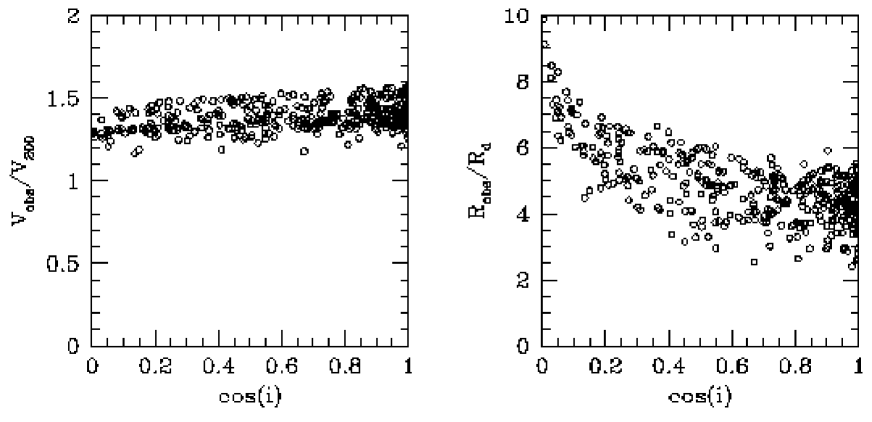
Figure 1.— The ratios $V_{\rm obs}/V_{200}$ (left panel) and $R_{\rm obs}/R_{d}$ (right panel) as functions of the cosine of the inclination angle for model galaxies with the parameters of model L5 (see Table 2). Here $R_{\rm obs}$ is defined as the radius where the projected surface density of the HI reaches a column density of $10^{20}{\rm cm}^{-2}$, and $V_{\rm obs}=V_{c}(R_{\rm obs})$. For disks seen close to edge-on ($i\simeq 90^{\rm o}$), $R_{\rm obs}$ becomes as large as $\sim 10R_{d}$. For close to face-on systems, $R_{\rm obs}/R_{d}\simeq 4.5$ with a considerable scatter. Despite this relatively large change in $R_{\rm obs}$, the ratio $V_{\rm obs}/V_{200}$ is almost independent of $i$. This indicates that $V_{\rm obs}$ is an accurate measure of the flat part of the rotation curve, and we therefore use $V_{\rm obs}$ and $V_{\rm flat}$ without distinction throughout the paper.

Figure 2.— Model TF relation for model S1 (SCDM with parameters set to obtain maximally bright galaxies). Open circles correspond to the model galaxies, and the solid line corresponds to the observed $K$-band TF relation of V97. Only galaxies with $-19\geq M_{K}-5{\rm log}h\geq-25$ are shown, which corresponds to the magnitude interval on which the empirical TF relation is based. The slope of the model TF relation is too shallow ($b=-8.9$ as compared to $b_{\rm obs}=-10.5$), and model galaxies are too faint at the bright end. Since galaxies are maximally bright, this rules against the SCDM model (see text).

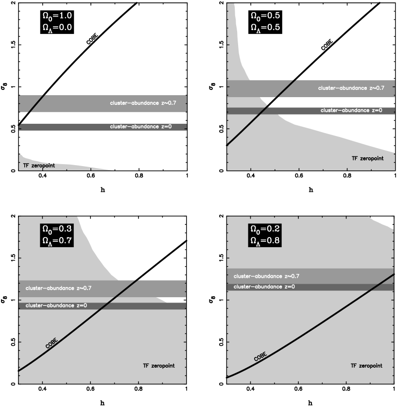
Figure 3.— Constraints on $\sigma_{8}$ and $h$ for four flat cosmologies with different values of $\Omega_{0}$. The light gray areas correspond to the parts of parameter space allowed by the TF zero-point. Cosmological models with $(\sigma_{8},h)$ in the white areas yield galaxies that are too faint. In addition, constraints are plotted from the 4 year data from the COBE DMR experiment (Bunn & White 1997; solid lines) and from the cluster abundances at $z=0$: $\sigma_{8}=(0.52\pm 0.04)\,\Omega_{0}^{-0.52+0.13\Omega_{0}}$ (Eke, Cole & Frenk 1996; dark gray bars) and $z\simeq 0.7$: $\sigma_{8}=(0.8\pm 0.1)\,\Omega_{0}^{-0.29}$ (Bahcall & Fan 1998; median gray bars). In a flat universe without cosmological constant (upper right panel) the TF zero-point imposes stringent constraints on $\sigma_{8}$ and $h$. In order for galaxies in this cosmology to be as bright as required by the TF relation, $\sigma_{8}\lesssim 0.08$ when $h=0.5$. This is in clear contradiction with the other constraints. Since a decrease of $\Omega_{0}$ induces an increase of the baryon fraction (i.e., we adopt $f_{\rm bar}=0.0125\,\Omega_{0}^{-1}h^{-2}$ throughout) , the TF constraints become less restrictive for lower values of the matter density. Combining all constraints suggests $\Omega_{0}\lesssim 0.3$.

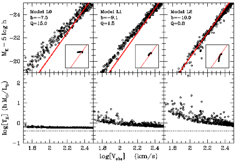
Figure 4.— The upper panels show TF relations for three models in a flat $\Lambda$CDM universe with $\Omega_{0}=0.3$ (symbols are the same as in Figure 2). All these models ignore feedback (i.e., $\epsilon_{\rm gf}=1$) and have all the mass that is eligible for star formation turned into stars over the lifetime of the galaxy (i.e., $f_{\rm SF}=1$). The models only differ in the value of $Q$ as indicated in the panels. In addition, the panels list the model ID and the slope of the best fitting TF relation. The small insets plot TF relations for model galaxies that only differ in $\lambda$ (all galaxies have $M_{200}=3\times 10^{11}h^{-1}\>{\rm M_{\odot}}$ and have a value of $\lambda$ drawn from the log-normal distribution of equation [7] with $\sigma_{\lambda}=0.6$). These insets show how $\sigma_{\lambda}$ contributes to the scatter (see discussion in § 6). The lower panels plot ${\rm log}(\Upsilon_{K})$ (equation [28]) as function of ${\rm log}(V_{\rm obs})$. The dotted lines correspond to $\Upsilon_{K}=\Upsilon_{K}^{*}=0.4\>{\rm M_{\odot}}/\>{\rm L_{\odot}}$. Lower mass systems require a significantly higher value of $\Upsilon_{K}$ than more massive galaxies in order to fit the observed slope. This can be accomplished by lowering $Q$ to $\sim 0.8$.

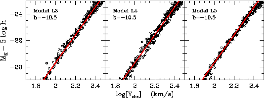
Figure 5.— Model TF relations for three $\Lambda$CDM3 models that all fit the empirical $K$-band TF relation of equation (3). Each of these models, however, represent a different class of physics. In model L3, the $K$-band stellar mass-to-light ratios are varied with mass to obtain $b=-10.5$. In model L4, the same is accomplished, but by adopting a power spectrum that is shallower than for CDM on the scale of galaxies. Finally, in model L5 feedback is included to tilt the TF relation to its observed slope.

Figure 6.— Model TF relations for three $\Lambda$CDM2 models (upper panels). The models differ only in the parameters describing star formation and feedback (see Table 2). The effects of these two physical processes are indicated in the panels in the two lower rows, where we plot $\epsilon_{\rm gf}$ (a measure of the feedback efficiency) and $f_{\rm SF}$ (a measure of the star formation efficiency) as functions of ${\rm log}(V_{\rm obs})$. If no feedback is taken into account, and all the mass eligible for star formation is turned into stars over the lifetime of the galaxy (panels on the left), galaxies are almost two magnitudes too bright. Models L7 and L8, in which feedback is taken into account, both provide good fits to the observed TF relation.

Figure 7.— Histogram of the normalized distribution of $c/c_{0}$ for model L5 with $\sigma_{z}=0.4$. Here $c_{0}$ is the halo concentration parameter predicted by the Press-Schechter formalism (see Navarro et al. 1997 for details). The solid curve represents the log-normal distribution of $c/c_{0}$ for halos without significant amounts of substructure as determined by Jing (1999) from high resolution $N$-body simulations (in Jing’s notation, we only included halos with ${\rm dvi}_{\rm max}<0.15$). Despite a small offset in the mean (Jing finds $\langle c\rangle\simeq 0.95c_{0}$), the two distributions agree well, and we conclude therefore that a standard deviation of $0.4$ in halo collapse redshifts is a good representation of the scatter in halo concentrations that owes to scatter in mass aggregation histories.

Figure 8.— Illustration of the build-up of scatter in the TF relation of model L5. Contrary to previous plots (i.e., Figures 2, 4, 5, and 6) we plot the TF relation over the entire range of $M_{K}$ of our model galaxies. This emphasizes the curvature present in the TF relation, and which owes mainly to the feedback. In the upper left panel, no intrinsic scatter is present. The small amount of scatter in the TF relation of $\sigma_{M}=0.06$ mag owes to the curvature. The upper right panel shows the same TF relation but now with $\sigma_{\lambda}=0.6$. The variance in halo spin parameters increases $\sigma_{M}$ to 0.13 mag. Setting $\Delta i=45^{\rm o}$ further increases the scatter to $\sigma_{M}=0.16$ mag (lower left panel). Finally, the addition of scatter in the halo collapse redshifts ($\sigma_{z}=0.4$) yields a total scatter of $\sigma_{M}=0.20$ mag.

Figure 9.— The shaded histogram plots the distribution of “observed” velocities (normalized to the mean) for model S1, but with $\Delta i=\sigma_{\lambda}=0$ and $\sigma_{z}=0.5$. The thick solid line corresponds to the same distribution, but calculated from the procedure used by Eisenstein & Loeb (1996). This latter method is based on the simplified assumptions of spherical accretion and isothermal halos, and predicts roughly twice the amount of scatter in the TF relation.

Figure 10.— The gas mass fraction $f_{\rm gas}$ (see equation [33]) as function of absolute $B$-band magnitude (left panels) and central disk surface brightness (right panels). Upper panels plot the data of McGaugh & de Blok (1997), while the panels in the lower three rows correspond to models L2, L5 and L8, as indicated. The data is based on $B$-band photometry, and we convert our models ($K$-band) to the $B$-band using $B-K=0.64-0.18(M_{K}-5{\rm log}h_{75})$ with $h_{75}=H_{0}/(75\>{\rm km}\,{\rm s}^{-1}\,{\rm Mpc}^{-1})$ (see Appendix A in van den Bosch & Dalcanton 1999). The thin solid lines have no physical meaning, but are plotted to facilitate a comparison between models and data. Model L5 yields gas mass fractions that are in excellent agreement with the data. The model reproduces the decrease of $f_{\rm gas}$ with increasing luminosity and surface brightness, and the absolute values of $f_{\rm gas}$ are in excellent agreement with the data of MB97. Models L2 and L8, on the other hand, predict gas mass fractions that are too large to be consistent with observations.

Table 1Parameters of cosmological models.

Model	$\Omega_{0}$	$\Omega_{\Lambda}$	$h$	$\sigma_{8}$	$f_{\rm bar}$	$t_{0}$	Clusters	COBE	RCs	TF
(1)	(2)	(3)	(4)	(5)	(6)	(7)	(8)	(9)	(10)	(11)
SCDM	$1.0$	$0.0$	$0.5$	$0.6$	$0.05$	$13.0$	Y	N	N	N
$\Lambda$CDM3	$0.3$	$0.7$	$0.7$	$1.0$	$0.085$	$13.5$	Y	Y	N	Y
$\Lambda$CDM2	$0.2$	$0.8$	$0.5$	$0.38$	$0.25$	$21.0$	N	Y	Y	Y

Note. — Column (1) lists the name of the CDM cosmology by which we refer to it in the text. Columns (2), (3), (4), and (5) list the matter density, $\Omega_{0}$, the density in the form of a cosmological constant, $\Omega_{\Lambda}=\Lambda/(3\,H_{0}^{2})$ (with $\Lambda$ the cosmological constant), the hubble parameter, $h=H_{0}/(100\>{\rm km}\,{\rm s}^{-1}\,{\rm Mpc}^{-1})$, and the rms mass variance on a scale of $8h^{-1}$ Mpc, $\sigma_{8}$. Column (6) lists the baryon fraction $f_{\rm bar}=\Omega_{\rm bar}/\Omega_{0}$ based on a baryon density of $\Omega_{\rm bar}=0.0125\,h^{-2}$ as required by nucleosynthesis constraints (e.g., Walker et al. 1991). Column (7) lists the age of the universe in Gyr. Columns (8) to (11) indicate whether the models are consistent with the observed cluster abundances, the COBE normalization, the observed rotation curves of spirals (RCs; see Navarro 1998), and the TF zero-point, respectively (see § 4 for details)

Table 2Parameters of models discussed in the text.

ID.	Cosmology	$Q$	$\Upsilon^{*}_{K}$	$n$	$A_{\rm SF}$	$\varepsilon_{\rm SN}^{0}$	$\nu$	$\zeta$	$b$	$\sigma_{M}$
(1)	(2)	(3)	(4)	(5)	(6)	(7)	(8)	(9)	(10)	(11)
S1	SCDM	$1.5$	$0.3$	$1.4$	$0.25$	$0.0$	$0.0$	$--$	$-8.9$	$0.15$
L0	$\Lambda$CDM3	$15.0$	$0.4$	$1.4$	$0.25$	$0.0$	$0.0$	$--$	$-7.5$	$0.28$
L1	$\Lambda$CDM3	$1.5$	$0.4$	$1.4$	$0.25$	$0.0$	$0.0$	$--$	$-9.1$	$0.18$
L2	$\Lambda$CDM3	$0.8$	$0.4$	$1.4$	$0.25$	$0.0$	$0.0$	$--$	$-10.0$	$0.23$
L3	$\Lambda$CDM3	$1.5$	$\propto(V_{200})^{-0.7}$	$1.4$	$0.25$	$0.0$	$0.0$	$--$	$-10.5$	$0.20$
L4	$\Lambda$CDM3	$1.5$	$0.4$	$1.4$	$0.25$	$0.0$	$0.0$	$0.26$	$-10.5$	$0.22$
L5	$\Lambda$CDM3	$1.5$	$0.4$	$1.4$	$0.25$	$0.05$	$-0.3$	$--$	$-10.5$	$0.16$
L6	$\Lambda$CDM2	$1.5$	$0.4$	$1.4$	$0.25$	$0.0$	$0.0$	$--$	$-9.0$	$0.19$
L7	$\Lambda$CDM2	$1.5$	$0.4$	$1.4$	$0.25$	$2.0$	$0.0$	$--$	$-10.6$	$0.13$
L8	$\Lambda$CDM2	$1.5$	$0.4$	$1.4$	$0.01$	$0.05$	$-2.6$	$--$	$-10.7$	$0.13$

Note. — Column (1) lists the model ID, by which we refer to it in the text. Column (2) lists the cosmological model used (see Table 1). Columns (3) and (4) list the value of the Toomre parameter, $Q$, and the $K$-band stellar mass-to-light ratio, $\Upsilon_{K}^{*}$, respectively. The star formation parameters $n$ and $A_{\rm SF}$ are listed in columns (5) and (6), respectively. Columns (7) and (8) list the feedback parameters $\varepsilon_{\rm SN}^{0}$ and $\nu$, respectively. Column (9) gives the parameter $\zeta$. This parameter is only defined for model L3; for all other models, the mass dependence of $c$ is determined from the CDM power spectrum. Finally, columns (10) and (11) list the slope $b$ and scatter $\sigma_{M}$ (in mag) of the TF relation for model galaxies with $-19\geq M_{K}-5{\rm log}h\geq-24$ and with $\sigma_{z}=0$

References

- (1) Aaronson, M., Huchra, J., & Mould, J. 1979, ApJ, 229, 1
- (2) Andredakis, Y. C., Peletier, R. F., & Balcells, M. 1995, MNRAS, 275, 874
- (3) Avila-Reese, V., Firmani, C., & Hernández, X. 1998, ApJ, 505, 37 (AFH98)
- (4) Bahcall, N. A., & Fan, X. 1998, ApJ, 504, 1
- (5) Barnes, J. E., & Efstathiou, G. 1987, ApJ, 319, 575
- (6) Baugh, C. M., Cole, S., & Frenk, C. S. 1996, MNRAS, 283, 1361
- (7) Blumenthal, G. R., Faber, S. M., Flores, R., & Primack, J. R. 1986, ApJ, 301, 27
- (8) Bruzual, G. A., & Charlot, S. 1993, ApJ, 405, 538
- (9) Bunn, E. F., & White, M. 1997, ApJ, 480, 6
- (10) Christodoulou, D. M., Shlosman, I., & Tohline, J. E. 1995, ApJ, 443, 551
- (11) Cole, S. 1991, ApJ, 367, 45
- (12) Cole, S., Aragón-Salamanca, A., Frenk, C. S., Navarro, J. F., & Zepf, S. E. 1994, MNRAS, 271, 781
- (13) Cole, S., & Lacey, S. 1996, A&A, 281, 716
- (14) Courteau, S. 1997, AJ, 114, 2402
- (15) Dalcanton, J. J., Spergel, D. N., & Summers, F. J. 1997, ApJ, 482, 659
- (16) Domínguez-Tenreiro, R., Tissera, P. B., & Sáiz, A. 1998, ApJ, 508, 123
- (17) Dubinski, J., & Carlberg, R. 1991, ApJ, 434 402
- (18) Efstathiou, G., Frenk, C. S., White, S. D. M., & Davis, M. 1988, MNRAS, 235, 715
- (19) Eisenstein, D. J., & Loeb, A. 1996, ApJ, 459, 432 (EL96)
- (20) Eke, V. R., Cole, S., & Frenk, C. S. 1996, MNRAS, 282, 263
- (21) Elizondo, D., Yepes, G., Kates, R., Müller, V., & Klypin, A. 1999, ApJ, 515, 525
- (22) Evrard, A. E. 1997, in Galaxy Scaling Relations: Origins, Evolution and Applications, ed. L. N. da Costa & A. Renzini (Springer-Verlag), p. 25
- (23) Evrard, A. E., Summers, F. J., & Davis, M. 1994, ApJ, 422, 11
- (24) Faber, S. M. 1982, in Astrophysical Cosmology: Proc Study Week on Cosmology and Fundamental Physics, ed. H.A. Brück, G.V. Coyne & M.S. Longair, (Vatican: Pontifical Sci Acad), p. 191
- (25) Fall, S. M. 1983, in IAU Symp. 100, Internal Kinematics and Dynamics of Galaxies, ed. E. Athanassoula (Dordrecht: Reidel), 391
- (26) Fall, S. M., & Efstathiou, G. 1980, MNRAS, 193, 189
- (27) Firmani, C., & Avila-Reese, V. 1998a, preprint (astro-ph/9803090)
- (28) Firmani, C., & Avila-Reese, V. 1998b, preprint (astro-ph/9810293)
- (29) Flores, R., Primack, J. R., Blumenthal, G. R., & Faber, S. M. 1993, ApJ, 412, 443
- (30) Frenk, C. S., White, S. D. M., Davis, M., & Efstathiou, G. 1988, ApJ, 327, 507
- (31) Gavazzi, G. 1993, ApJ, 419, 469
- (32) Gavazzi, G., Pierini, D., & Boselli, A. 1996, A&A, 312, 397
- (33) Haynes, M. P., Giovanelli, R., Chamareux, P., da Costa, L. N., Freudling, W., Salzer, J. J., Wegner, G. 1999, AJ, 117, 2039
- (34) Heavens, A. F., & Jiminez, R, 1999, MNRAS, 305, 770
- (35) Hernquist, L. 1990, ApJ, 356, 359
- (36) Heyl, J. S., Cole, S., Frenk, C. S., Navarro, J. F. 1995, MNRAS, 274, 755
- (37) Hoyle, F. 1953, ApJ, 118, 513
- (38) Jing, Y. P. 1999, preprint (astro-ph/9901340)
- (39) Kauffmann, G. 1996, MNRAS, 281, 475
- (40) Kauffmann, G., White, S. D. M., & Guiderdoni, B. 1993, MNRAS, 264, 201
- (41) Kennicutt, R. C. Jr. 1989, ApJ, 344, 685
- (42) Kennicutt, R. C. Jr. 1998, ApJ, 498, 541
- (43) Klypin, A. A., Kravtsov, A. V., Valenzuela, O., & Prada, F. 1999, preprint (astro-ph/9901240)
- (44) Kravtsov, A. V., Klypin, A. A., Bullock, J. S., & Primack, J. R. 1998, ApJ, 502, 48
- (45) Lacey, C., & Silk, J. 1991, ApJ, 381, 14
- (46) Lacey, C., & Cole, S. 1993, MNRAS, 262, 627
- (47) Lacey, C., Guiderdoni, B., Rocca-Volmerange, B., & Silk, J. 1993, ApJ, 402, 15
- (48) Lemson, G., & Kauffmann, G. 1999, MNRAS, 302, 111
- (49) Mac Low, M.-M., & Ferrara, A. 1999, ApJ, 513, 142
- (50) Maraston, C. 1998a, MNRAS, 300, 872
- (51) Maraston, C. 1998b, preprint (astro-ph/9808263)
- (52) Matthews, L. D., van Driel, W., Gallagher, J. S. III. 1998, AJ, 116, 2196
- (53) McGaugh, S. S., & de Blok, W. J. G. 1997, ApJ, 481, 689 (MB97)
- (54) McGaugh, S. S., & de Blok, W. J. G. 1998a, ApJ, 499, 41
- (55) Mo, H. J., Mao, S., & White, S. D. M. 1998, MNRAS, 295, 319
- (56) Moore, B., Governato, F., Quinn, T., Stadel, J., & Lake, G. 1998, ApJ, 499, L5
- (57) Moore, B., Ghigna, S., Governato, F., Lake, G., Quinn, T., Stadel, J., & Tozzi, P. 1999, Nature, in press
- (58) Natarajan, P. 1999, ApJ, 512, 105
- (59) Navarro, J. F. 1998, preprint (astro-ph/9807084)
- (60) Navarro, J. F., & White, S. D. M. 1994, MNRAS, 267, 401
- (61) Navarro, J. F., Frenk, C. S., & White, S. D. M. 1995, MNRAS, 275, 720
- (62) Navarro, J. F., Frenk, C. S., & White, S. D. M. 1996, ApJ, 462, 563
- (63) Navarro, J. F., Frenk, C. S., & White, S. D. M. 1997, ApJ, 490, 493
- (64) Ostriker, J. P., & Peebles, P. J. E. 1973, ApJ, 186, 467
- (65) Peletier, R. F., & Balcells, M. 1997, New Astronomy, 1, 349
- (66) Pierce, M. J., & Tully, R. B. 1988, ApJ, 330, 579
- (67) Pierce, M. J., & Tully, R. B. 1992, ApJ, 387, 47
- (68) Quirk, W. J. 1972, ApJ, 176, L9
- (69) Ryden, B. S. 1988, ApJ, 329, 589
- (70) Salucci, P., Frenk, C. S., & Persic, M. 1993, MNRAS, 262, 392
- (71) Scalo, J. N. 1986, Fundam. Cosmic Phys., 11, 1
- (72) Schmidt, M. 1959, ApJ, 129, 243
- (73) Silk, J. 1997, ApJ, 481, 703
- (74) Somerville, R. S., & Primack, J. R. 1998, preprint (astro-ph/9802268)
- (75) Sprayberry, D., Bernstein, G. M., Impey, C. D., & Bothun, G. D. 1995, ApJ, 438, 72
- (76) Steinmetz, M., & Müller, E. 1994, A&A, 268, 391
- (77) Steinmetz, M., & Navarro, J. F. 1999, ApJ, 513, 555
- (78) Stil, J. M., & Israel, F. P. 1998, preprint (astro-ph/9810151)
- (79) Syer, D., Mao, S., & Mo, H. J. 1999, MNRAS, 305, 357
- (80) Tissera, P. B., Lambas, D. G., & Abadi, M. G. 1997, MNRAS, 286, 384
- (81) Toomre, A. 1964, ApJ, 139, 1217
- (82) Tormen, G., Bouchet, F. R., & White, S. D. M. 1997, MNRAS, 286, 865
- (83) Tóth, G., & Ostriker, J. P. 1992, ApJ, 389, 5
- (84) Tully, R. B., & Fisher, J. R. 1977, A&A, 54, 661
- (85) Tully, R. B., Mould, J. & Aaronson, M. 1982, ApJ, 257, 527
- (86) Tully, R. B., Verheijen, M. A. W., Pierce, M. J., Huang, J., & Wainscoat, R. J., 1996, AJ, 112, 2471
- (87) van den Bosch, F. C. 1998, ApJ, 507, 601
- (88) van den Bosch, F. C. 1999, in The Formation of Bulges, eds. C. M. Carollo, H. C. Ferguson, R. F. G. Wyse (Cambridge: Cambridge University Press), in press (astro-ph/9901423)
- (89) van den Bosch, F. C., & Dalcanton, J. J. 1999, ApJ, submitted (paper II)
- (90) van der Kruit, P. C. 1987, A&A, 173, 59
- (91) Verheijen, M. A. W. 1997, PhD Thesis, University of Groningen (V97)
- (92) Visvanathan, N. 1981, A&A, 100, L20
- (93) Warren, M. S., Quinn, P. J., Salmon, J. K., & Zurek, W. H. 1992, ApJ, 399, 405
- (94) Walker, T. P., Steigman, G., Schramm, D. N., Olive, K. A., & Kang, H.-S. 1991, ApJ, 376, 51
- (95) White, S. D. M. 1997, in Galaxy Scaling Relations: Origins, Evolution and Applications, eds. L. N. da Costa & A. Renzini (Springer-Verlag)
- (96) White, S. D. M., & Rees, M. J. 1978, MNRAS, 183, 341
- (97) White, S. D. M., & Frenk, C. S. 1991, ApJ, 379, 52
- (98) Wyse, R. 1982, MNRAS, 199, 1P
- (99) Zwaan, M. A., van der Hulst, J. M., de Blok, W. J. G., & McGaugh, S. S. 1995, MNRAS, 273, L35