The X-ray variability of the Seyfert 1 galaxy MCG$-$6-30-15 from long ASCA and RXTE observations

Abstract

We present an analysis of the long Rossi X-ray Timing Explorer (RXTE ) observation of the Seyfert 1 galaxy MCG$-$6-30-15, taken in July 1997. We have earlier used the data to place constraints for the first time on the iron abundance - reflection fraction relationship, and now expand the analysis to investigate in detail the spectral X-ray variability of the object. Our results show that the behaviour is complicated. We find clear evidence from colour ratios and direct spectral fitting that changes to the intrinsic photon index are taking place. In general, spectral hardening is evident during periods of diminished intensity, and in particular, a general trend for harder spectra is seen in the period following the hardest RXTE flare. Flux-correlated studies further show that the 3$-$10 keV photon index $\Gamma_{3-10}$ steepens while that in the 10–20 keV band, $\Gamma_{10-20},$ flattens with flux. The largest changes come from the spectral index below 10 keV; however, changes in the intrinsic power law slope (shown by changes in $\Gamma_{3-10}$), and reflection (shown by changes in $\Gamma_{10-20}$) both contribute in varying degrees to the overall spectral variability. We find that the iron line flux $F_{\rm K\alpha}$ is consistent with being constant over large time intervals on the order of days (although the ASCA and RXTE spectra show that $F_{\rm K\alpha}$ changes on shorter time intervals of order $\mathrel{\hbox to0.0pt{\lower 3.0pt\hbox{$\sim$}\hss}\raise 2.0pt\hbox{$<$}}$ 10 ks), and equivalent width which anticorrelates with the continuum flux, and reflection fraction. A possible interpretation for the iron line flux constancy and the relative Compton reflection increase with flux from the flux-correlated data is an increasing ionization of the emitting disk surface, while spectral analysis of short time intervals surrounding flare events hint tentatively at observed spectral responses to the flare. We present a simple model for partial ionization where the bulk of the variability comes from within $6r_{g}$. Temporal analysis further provides evidence for possible time ($\mathrel{\hbox to0.0pt{\lower 3.0pt\hbox{$\sim$}\hss}\raise 2.0pt\hbox{$<$}}$ 1000s) and phase ($\phi\sim 0.6$ rad) lags. Finally, we report an apparent break in the power density spectrum ($\sim 4-5\times 10^{-6}$ Hz) and a possible 33 hour period. Estimates for the mass of the black hole in MCG$-$6-30-15 are discussed in the context of spectral and temporal findings.

1 INTRODUCTION

Observational and theoretical progress over the past decade have greatly improved our understanding of accreting black holes in Seyfert galaxies. Time-averaged X-ray spectra reveal a hard power-law continuum with a broad iron line and continuum reflection components (Pounds et al 1990; Nandra & Pounds 1994; Tanaka et al 1995; Nandra et al 1997). The power-law emission is produced by thermal Comptonization in $\sim 100$ keV hot gas (Zdziarski et al 1994) above a thin accretion disc, which causes the reflection (Guilbert & Rees 1988; Lightman & White 1988; George & Fabian 1991; Matt, Perola & Piro 1991).

Spectral variability in some objects show that the emission is produced in flarelike events which may move about over the inner accretion flow. The information from such variability is complex and its interpretation is not necessarily straightforward. Barr & Mushotzky (1986) and Wandel & Mushotzky (1986), by invoking the criterion for the fastest doubling time found in observations of AGN, demonstrate that a correlation between the X-ray luminosity and variability time scales exist and use this to place upper limits on the black hole masses in their sample of AGN observed with a slew of X-ray telescopes that include Ariel V, HEAO-1, and the Einstein observatory. Such a method however has been criticized for its dependence on data quality and coverage (Lawrence et al. 1987; Mchardy & Czerny 1987). It does nevertheless provide a strong limit on the size of the emitting region. For example, Reynolds et al. (1995) and Yaqoob et al. (1997) have reported a factor of 1.5 increase in flux in as little as 100s in MCG$-$6-30-15.

Others have resorted to employing power density spectrum (PDS) techniques (and variants thereof) as potential black hole mass estimators (e.g. Edelson & Nandra 1999 for NGC3516; Nowak & Chiang 1999 for MCG$-$6-30-15; Hayashida et al. 1998 introduces the normalized power spectrum density (NPSD) for their sample of AGN observed with Ginga). However, even this is not without its caveats. X-ray variability studies of AGNs thus far (with the exception of IRAS18325-5926; Iwasawa et al. 1998) has shown that the power-law spectrum is essentially chaotic with no characteristic period. The problem of unevenly sampled data streams, characteristic of X-ray observations of AGN, is overcome by the solution of Lomb (1976) and Scargle (1982; see Press et al 1992).

Others still have searched for time lags and leads using cross correlation function techniques. However, the problem associated with unevenly sampled data is still a concern, and has been addressed by e.g. Edelson & Krolik (1988), Yaqoob et al (1997), Reynolds (1999), and in this paper.

MCG$-$6-30-15 is a bright nearby (z=0.0078) Seyfert 1 galaxy that has been extensively studied by every major X-ray observatory since its identification. A recent study that takes advantage of the high energy and broad-band coverage of RXTE by Lee et al. (1998, 1999) with respectively a 50 ks observation in 1996, and 400 ks 1997 observation have confirmed the clear existence of a broad iron line and reflection component in this object. A previous study by Iwasawa et al. (1996) (hereafter I96) using a 4.5 day observation with ASCA revealed the iron line profile to be variable, which is confirmed in this long 1997 ASCA observation (Iwasawa et al. 1999, hereafter I99) which was observed simultaneously with RXTE . Additionally, Lee et al. (1999) have been able to constrain the iron abundance - reflection fraction relation for the first time using the RXTE observation. Guainazzi et al. (1999) give good bounds on the high energy cutoff of the continuum from a BeppoSAX observation of MCG$-$6-30-15.

We investigate in this paper changes in the direct and reflected components with our simultaneous RXTE and ASCA observations spanning a good time interval of $\approx$ 400 ks, in order to speculate on possible causes for variability. In Section 3, we investigate rapid variability with colour ratios. This is followed in Section 4 by flux-correlated studies, and a detailed analysis of the time intervals surrounding the bright ASCA and RXTE flare shown in Fig. 1. In Section 5, we shift gears to temporal studies and search (using cross-correlation techniques) for the presence of time lags and leads, in order to better understand the physical processes that may give rise to each other. We discuss in Section 6 tentative evidence for the presence of a possible 33 hour period, and break in the power spectrum. Finally, we discuss the spectral and temporal findings in Section 7. In particular, we discuss the challenge that spectral findings may pose to current models for reflection by cold material, and implications from temporal studies for placing constraints on the size of the emitting region and mass of the black hole in MCG$-$6-30-15. We present also a simple model to explain some of our enigmatic spectral findings. We conclude in Section 8 with a summary of the pertinent findings from this study.

2 Observations

MCG$-$6-30-15 was observed by RXTE over the period from 1997 Aug 4 to 1997 Aug 12 by both the Proportional Counter Array (PCA) and High-Energy X-ray Timing Experiment (HEXTE) instruments. We note that good data covered $\sim$400 ks, even though the RXTE observation spanned $\sim$700 ks. It was simultaneously observed for $\rm\sim 200~{}ks$ by the ASCA Solid-state Imaging Spectrometers (SIS) over the period 1997 August 3 to 1997 August 10 with a half-day gap part way through the observation. We concentrate only on the RXTE PCA observations in this paper.

2.1 Data Analysis

We extract PCA light curves and spectra from only the top Xenon layer using the ftools 4.2 software. The light curves were extracted with the default 16s time bins for Standard 2 PCA data time resolution. Data from PCUs 0, 1, and 2 are combined to improve signal-to-noise at the expense of slightly blurring the spectral resolution. Data from the remaining PCUs (PCU 3 and 4) are excluded because these instruments are known to periodically suffer discharge and are hence sometimes turned off.

Good time intervals were selected to exclude any earth or South Atlantic Anomaly (SAA) passage occulations, and to ensure stable pointing. We also filter out electron contamination events.

We generate background data using pcabackest v2.0c in order to estimate the internal background caused by interactions between the radiation/particles and the detector/spacecraft at the time of observation. This is done by matching the conditions of observations with those in various model files. The model files used are the L7-240 background models which are intended to be specialized for application to faint sources with count rate less than 40 $\rm cts\,s^{-1}\,PCU^{-1}$.

The PCA response matrix for the RXTE data set was created using pcarsp v2.36. Background models and response matrices are representative of the most up-to-date PCA calibrations.

Figure 1: Background-subtracted light curve of MCG$-$6-30-15 for observations with 3 PCUs in the 2-60 keV band for the RXTE PCA, and 0.6$-$10 keV ASCA SIS. The epoch of the start and stop times for RXTE and ASCA respectively is 1997 August 4, 03:27:06 (UT) and 1997 August 12, 12:34:14 (UT) (RXTE ), and 1997 August 3 to 1997 August 10 (ASCA ). Light curves are binned using 256s time intervals. The intervals corresponding to the ASCA and RXTE flares are further subdivided and discussed in depth in Section 4.3.

Figure 1 shows the background subtracted light curve for ASCA and RXTE , with 256s binning. The time intervals corresponding to the ASCA and RXTE flares are decomposed further and analyzed in depth in Section 4.3. Significant variability can be seen in both light curves on short and long timescales. Flare and minima events are seen to correlate temporally in both light curves.

3 Rapid Variability

Intraday variability has been seen in most quasars and AGNs; in MCG$-$6-30-15, rapid X-ray variability on the order of 100 s has been reported by a number of workers (e.g. Reynolds et al. 1995; Yaqoob et al. 1997). These significant luminosity changes on time scales as short as minutes can have strong implications for restricting the size of the emitting region, and efficiency of the central engine. Colour ratios are good tools for discerning the processes that may give rise to these rapid variability effects. For the purposes of our study, we define the following count rate hardness ratios in order to assess the processes that may give rise to variability :

$$R_{1}=\frac{5-7~{}keV}{3-4.5~{}keV}$$ (1)

$$R_{2}=\frac{7.5-10~{}keV}{3-4.5~{}keV}\qquad\mbox{, }\qquad R_{3}=\frac{7.5-10~{}keV}{5-7~{}keV}$$ (2)

$$R_{4}=\frac{10-20~{}keV}{3-4.5~{}keV}\qquad\mbox{, }\qquad R_{5}=\frac{10-20~{}keV}{5-7~{}keV}$$ (3)

$$\qquad\mbox{}\qquad R_{6}=\frac{10-20~{}keV}{7.5-10~{}keV}$$

We expect the reflection component to dominate above 10 keV. At the lower energies, the dominant features include the iron line between 5.5-6.5 keV and the warm absorber below 2 keV. We note also that the iron line contribution to the overall flux in the 5-7 keV band is only $\sim$ 15%, and hence be hereafter referred to as the iron line band.

Hardness ratio	$\chi_{\nu}^{2}$
R1	3.7
R2	3.25
R3	0.95
R4	4.42
R5	1.95
R6	1.24

Table 1: Assessment for amount/absence of variability for the hardness ratios shown on the left panels of Figs. 2$-$4. $\chi_{\nu}^{2}$ is evaluated for 138 degrees of freedom.

The $\rm R_{1}$ assessment of the (5-7 keV) iron line band versus (3-4.5 keV) lower continuum (Fig. 2a) shows that the source is intrinsically harder during the minima. Similarly, $\rm R_{2}$ hardness ratio of the (7.5-10 keV) upper continuum to the (3-4.5 keV) lower continuum reveals a similar trend (Fig. 3a); likewise, $\rm R_{4}$ assessment of the (10-20 keV) reflection hump and (3-4.5 keV) lower continuum (Fig. 4a). $\rm R_{3}$, $\rm R_{5}$, $\rm R_{6}$ show no obvious trends (respectively Figs. 3b,4b,4c) from count-rate versus hardness ratio plots, although subtle correlations can be seen in the time versus hardness ratio plots. In particular Figs. 4b and 4c show dramatic hardening of the spectrum during the time periods following the RXTE flare. (We mark the beginning of the ASCA and RXTE flares respectively with ‘A’ and ‘X’ in the light curves shown in Figs. 2$-$4.) In order to further quantify the amount / absence of variablity, we apply a $\chi^{2}$ test to the hardness ratio trends as shown in the left panels of Figs. 2$-$4. Table 1 details these results for 138 degrees of freedom.

3.1 The unusual properties of the deep minimum period following the hard RXTE flare

We mark the regions corresponding to the ASCA and RXTE flare events in Figs. 2$-$4. The time span corresponding to the ASCA and RXTE flares were chosen in order that the times surrounding the flares and minimum (following said flare) can be compared. The spectral behaviour during these periods is thoroughly investigated in Section 4.3. For present purposes, we draw the reader’s attention to the deep minimum immediately following the bright RXTE flare. (The general location of this minimum in the light curve is labeled with ‘DM’ in Figs. 2$-$4.) Despite the hardness ratio results discussed previously (e.g. no obvious trends seen in $\rm R_{3}$, $\rm R_{5}$, $\rm R_{6}$), the spectrum during this time period always hardens in all colours, whereas this is not necessarily the case with the other minima events (e.g. the deep minimum following the soft ASCA flare). In addition, it is not clear whether the spectrum reaches its lowest minimum slightly before or after an observed hardening.

We also bring attention (by means of a horizontal line through the hardness ratio versus time plots in Figs. 2$-$4) to the general trend for harder spectra in the $\sim$ 260 ks time period that begins with the RXTE flare.

3.2 Possible causes of Hardness Ratio Variability

Many complicated processes contribute to the overall temporal and spectral behaviour of an AGN. It is necessary to disentangle these components in order to assess the physical processes that are responsible for the observed variability phenomenon. Effects due to reprocessing are significant only at the higher energies, the (10-20 keV) band being the most sensitive probe of any subtle changes in the reflection component. Martocchia & Matt (1996) suggested that gravitational bending/focusing as the X-ray source gets closer to the black hole will enhance the amount of reflection. Therefore, it is possible that flares closer to the hole during the minima can enhance the amount of reflection, through increased beaming of the emission towards the disk. We conclude however from the combined hardness ratio findings described thus far that the spectral hardening during periods of diminished intensity point largely to changes in the intrinsic photon index $\Gamma$ being the main culprit for the observed spectral variability. We are led to this conclusion because spectral changes are seen in all bands, which is most likely to be due to changes in the spectral index. In other words, we may be seeing the effects of changes in the coronal temperature affecting the intrinsic power law slope, or that changes in $\Gamma$ are due to coverage of flares such that we are observing the effects of flares occurring at different heights (e.g. Poutanen & Fabian 1999). However, as we shall now show, direct spectral analysis reveals a more complex situation.

     

Figure 2: Hardness ratio plotted against time and countrate for the iron line band (5-7 keV) versus lower continuum (3-4.5 keV). Light curves are binned into 5000s intervals, and represent the sum of the light curve of the two energy bands being compared.

           

Figure 3: Hardness ratio plots against time and count rate of the upper continuum (7.5-10 keV) versus (a) lower continuum (3-4.5 keV) and (b) iron line band (5-7 keV). Light curves are binned into 5000s intervals, and represent the sum of the light curve of the two energy bands being compared..

                 

Figure 4: Hardness ratio plotted against time and count rate for the reflection hump (10-20 keV) versus (a) the lower continuum (3-4.5 keV), (b) iron line band (5-7 keV), and (c) upper continuum (7.5-10 keV). Light curves are binned into 5000s intervals, and represent the sum of the light curve of the two energy bands being compared..

4 Spectral Fitting

Having established that variability effects are many, we next investigate spectral changes in time sequence in order to obtain a better understanding of variability phenomena between the different flux states with particular emphasis on the flares and deep minima. Data analysis is restricted to the 3 to 20 keV PCA energy band. The lower energy restriction at 3 keV is selected in order that the necessity for modelling photoelectric absorption due to Galactic ISM material, or the warm absorber that are known to be present in this object is removed. (Lee et al. 1999 have shown that effects due to the warm absorber at 3 keV are negligible for this data set.)

4.1 Spectra selected in time sequence and by flux

We choose the time intervals (Fig. 1) in order to contrast and study the different variability states. They are defined such that intervals i1 and i6 correspond to the two RXTE deep minima, and intervals i2 and i7 for the relatively calm periods following these minima, and i5 a flare event for comparison. We investigate in detail in Section 4.3 the times surrounding the RXTE counterpart of the soft ASCA flare, and the hard flare observed by RXTE (unfortunately missed by ASCA ), as depicted in Fig. 1 and subsequently in Figs 9, and 11. Both the ASCA and RXTE light curves for the full observation are shown in Fig. 1.

We also separate the data according to flux in order to assess whether a clear picture can be developed of the dominant processes that may be at work for a given flux state. To do so, we separate the 400 ks observation by flux, with f2 and f3 being the intermediate states between the lowest f1 ($\rm 2.84\times 10^{-11}$ ${\rm\thinspace erg}{\rm\thinspace cm}^{-2}{\rm\thinspace s}^{-1}\,$), and highest f4 ($\rm 4.79\times 10^{-11}$ ${\rm\thinspace erg}{\rm\thinspace cm}^{-2}{\rm\thinspace s}^{-1}\,$) fluxes. Properties of these flux levels (in the 2-60 keV, and 3-20 keV energy bands), and i1$-$i7 intervals are detailed respectively in Table 2, and Table 7.

4.2 Temporal Variability and Spectral Features

A nominal fit to the entire data set (ie. ASCA , RXTE PCA and HEXTE) demonstrated the clear existence of a redshifted broad iron K$\alpha$ line at $\sim$ 6.0 keV and reflection hump between 20 and 30 keV as shown in Lee et al. (1998, 1999). In general, fits to the solar abundance models of George & Fabian 1991 (hereafter GF91) are better than simple power law fits and further reinforce the preference for a reflection component. Since the reflected continuum does not contribute significant flux to the observed spectrum below 10 keV, a simple power law and iron line fit to the data below 10 keV will reveal changes in the intrinsic power-law of the X-ray source. If indeed spectral variability is due to changes in the intrinsic power law slope which would implicate changes in the conditions of the X-ray emitting corona, we should see noticeable changes in the values of $\Gamma_{(3-10)}$ between the different temporal states. However, because reflection only significantly affects energies above 10 keV, changes seen in $\Gamma_{(10-20)}$ would suggest that variability may be due to the amount of reprocessing. (We have tested this premise by comparing simulated spectra in xspec using the pexrav model and find that the overall flux contribution from reflection alone is $>$ 60 per cent above 10 keV.) This would have strong implications for geometry (ie. where the direct X-ray flares are partially obscured), motion of the source (eg. Reynolds & Fabian 1997; Beloborodov 1998), or gravity (light-bending effects that will beam/focus more of the emission down towards the disk; Martocchia & Matt 1996).

4.2.1 The different flux states

We first investigate whether a correlation exists between flux and the various fit parameters, and in particular whether changes in reflection are dramatic. We do so by first fitting a simple model that consists of a power law and redshifted Gaussian to the 3-10 keV band, and comparing that with a power law fit to the 10-20 keV band. In doing so, we find that while the intrinsic 3-10 keV power law slope increases, $\Gamma_{10-20}$ appears to flatten with increasing flux (Fig. 5). Additionally, the iron $\rm K\alpha$ flux $F_{\rm K\alpha}$ does not change with any statistical significance while the flux between the lowest f1 and highest f4 flux nearly doubles (Table 2); similar results for the constancy of the iron line in MCG$-$6-30-15 was noted by McHardy et al. (1998), and by Chiang et al. (1999) for Seyfert 1 galaxy NGC5548. The ratio plot of data-to-model using a simple power law fit to the 3-20 keV data clearly illustrates the difference in the line and reflection component between the lowest and highest flux states in Fig. 7a.

Change in $\Gamma$ for different states of MCG$-$6-30-15
Flux	$\rm\Gamma_{3-10}^{a}$	$F_{\rm K\alpha}^{b}$	$\rm\Gamma_{10-20}^{c}$	$W_{\rm K\alpha}^{d}$	$\rm Flux^{e}$	Exposure	2-60 keV	Flux cuts	Time range
Levels		${\rm\thinspace ph}{\rm\thinspace cm}^{-2}{\rm\thinspace s}^{-1}\,$		$\rm eV$	(3$-$10 keV)	$\rm 10^{4}$ s	$\rm ct$ $\rm s^{-1}$	$\rm ct$ $\rm s^{-1}$	$\rm 10^{4}s$
f1	1.91 $\pm$ 0.02	$1.81^{+0.16}_{-0.14}$	1.99 $\pm$ 0.10	$466^{+41}_{-36}$	2.84	7.8	9.89 $\pm$ 0.34	f $<$ 12	full
f2	1.93 $\pm$ 0.02	$1.89^{+0.19}_{-0.17}$	1.65 $\pm$ 0.09	$399^{+39}_{-37}$	3.44	5.7	13.03 $\pm$ 0.41	$\rm 12\leq f<14$	full
f3	1.95 $\pm$ 0.01	$1.72^{+0.14}_{-0.14}$	1.55 $\pm$ 0.07	$313^{+25}_{-25}$	3.94	7.7	15.43 $\pm$ 0.36	$\rm 14\leq f<17$	full
f4	1.98 $\pm$ 0.01	$1.85^{+0.19}_{-0.17}$	1.48 $\pm$ 0.07	$272^{+28}_{-28}$	4.79	6.2	19.33 $\pm$ 0.40	$\rm f\geq 17$	full

Table 2: Results are quoted from simple power law fits. ^a Power-law photon index for 3 keV $<$ E $<$ 10 keV. ^b Flux of iron emission line in units of $10^{-4}$ ${\rm\thinspace ph}{\rm\thinspace cm}^{-2}{\rm\thinspace s}^{-1}\,$. ^c Power-law photon index for 10 keV $<$ E $<$ 20 keV. ^d Equivalent width of the iron emission line. ^e 3-10 keV flux in units of $10^{-11}$ ${\rm\thinspace erg}{\rm\thinspace cm}^{-2}{\rm\thinspace s}^{-1}\,$Intervals f1-f4 correspond to the full time-averaged spectrum separated according to flux. Count rates are given for the 2-60 keV energy band of the RXTE PCA.

Spectral Fits using power-law with reflection model for different flux states of MCG$-$6-30-15
Data	$\rm{}^{a}\Gamma_{4-20}$	$\rm{}^{b}A$	$\rm{}^{c}refl$	$\rm{}^{d}LineE$	$\rm{}^{e}\sigma$	${}^{f}F_{\rm K\alpha}$	$\rm{}^{g}W$ (eV)	$\rm{}^{h}Flux$	$\rm{}^{i}\chi^{2}$
f1	$1.88^{+0.03}_{-0.03}$	$1.16^{+0.03}_{-0.04}$	$0.35^{+0.15}_{-0.16}$	$6.04^{+0.05}_{-0.05}$	$0.54^{+0.07}_{-0.06}$	$1.50^{+0.11}_{-0.12}$	$375^{+28}_{-30}$	4.61	76
f2	$1.97^{+0.03}_{-0.03}$	$1.57^{+0.05}_{-0.05}$	$0.91^{+0.22}_{-0.20}$	$6.03^{+0.07}_{-0.07}$	$0.54^{+0.09}_{-0.10}$	$1.31^{+0.16}_{-0.16}$	$261^{+31}_{-31}$	5.73	44
f3	$2.01^{+0.03}_{-0.02}$	$1.91^{+0.05}_{-0.05}$	$1.10^{+0.19}_{-0.16}$	$6.05^{+0.06}_{-0.06}$	$0.39^{+0.09}_{-0.10}$	$0.96^{+0.12}_{-0.11}$	$167^{+21}_{-19}$	6.58	34
f4	$2.07^{+0.03}_{-0.02}$	$2.51^{+0.09}_{-0.05}$	$1.37^{+0.23}_{-0.14}$	$5.98^{+0.09}_{-0.10}$	$0.36^{+0.14}_{-0.21}$	$0.72^{+0.14}_{-0.19}$	$98^{+19}_{-26}$	8.03	35

Table 3: ^a Power-law photon index. ^b Power-law flux at 1 keV, in units of $10^{-3}$ ${\rm\thinspace ph}{\rm\thinspace cm}^{-2}{\rm\thinspace s}^{-1}{\rm\thinspace keV}^{-1},$ ^c Reflective fraction = $\Omega/2\pi$. ^d Energy of the iron $K\alpha$ emission line. ^e Line width in units of eV. ^f Flux of iron emission line in units of $10^{-4}$ ${\rm\thinspace ph}{\rm\thinspace cm}^{-2}{\rm\thinspace s}^{-1}\,$. ^g Equivalent width of the emission line. ^h 3-20 keV flux in units of $10^{-11}$ ${\rm\thinspace erg}{\rm\thinspace cm}^{-2}{\rm\thinspace s}^{-1}\,$. ⁱ $\chi^{2}$ for 39 degrees of freedom.

Spectral Fits using power-law with edge model for different flux states of MCG$-$6-30-15
Data	$\rm{}^{a}\Gamma_{3-10}$	$\rm{}^{b}E_{\rm K\alpha}$	$\rm{}^{c}\sigma$	${}^{d}F_{\rm K\alpha}$	$\rm{}^{e}W_{\rm K\alpha}$ (eV)	${}^{f}\rm E_{edge}(keV)$	${}^{g}\tau$	$\rm{}^{h}\chi^{2}$
f1	$1.83^{+0.03}_{-0.04}$	$6.12^{+0.08}_{-0.07}$	$0.65^{+0.11}_{-0.09}$	$1.59^{+0.17}_{-0.20}$	$406^{+43}_{-51}$	$7.0+0.20$	$0.13^{+0.06}_{-0.07}$	15
f2	$1.84^{+0.03}_{-0.04}$	$6.16^{+0.11}_{-0.04}$	$0.65^{+0.16}_{-0.11}$	$1.56^{+0.43}_{-0.22}$	$325^{+90}_{-46}$	$7.0+0.15$	$0.15^{+0.07}_{-0.05}$	23
f3	$1.89^{+0.03}_{-0.02}$	$6.13^{+0.06}_{-0.06}$	$0.53^{+0.09}_{-0.10}$	$1.43^{+0.18}_{-0.20}$	$259^{+33}_{-36}$	$7.0+0.23$	$0.10^{+0.40}_{-0.40}$	13
f4	$1.92^{+0.02}_{-0.02}$	$6.10^{+0.08}_{-0.08}$	$0.60^{+0.12}_{-0.13}$	$1.46^{+0.43}_{-0.23}$	$214^{+63}_{-34}$	$7.0+0.16$	$0.11^{+0.04}_{-0.03}$	13

Table 4: ^a Power-law photon index. ^b Energy of the iron K$\alpha$ emission line. ^c Line width in units of keV. ^d Flux of iron emission line in units of $10^{-4}$ ${\rm\thinspace ph}{\rm\thinspace cm}^{-2}{\rm\thinspace s}^{-1}\,$. ^e Equivalent width of the emission line (eV). ^f Energy of absorption edge (redshifted to z=0.0078 appropriate for MCG$-$6-30-15) in units of keV. ^g Maximum value for the optical depth at threhold energy. ^h $\chi^{2}$ for 12 degrees of freedom.

Having demonstrated the existence of a strong reflection component in Fig. 7a, and assessed its nature with more complicated fits in Lee et al. (1999) for this data set, we next investigate the features of reflection in detail for the different fluxes by fitting the data with a multicomponent model that includes the reflected spectrum. The underlying continuum is fit with the model pexrav which is a power law with an exponential cut off at high energies reflected by an optically thick slab of neutral material (Magdziarz & Zdziarski 1995). We fix the inclination angle of the reflector at $30^{\circ}$ so as to agree with the disk inclination one obtains when fitting accretion disk models to the iron line profile as seen by ASCA (Tanaka et al. 1995). Due to the strong coupling between the fit parameters of $\Gamma$, abundances, and reflection, we fix the low-Z and iron abundance respectively at 0.5 and 2 solar abundances as determined by Lee et al. (1999) for the fits presented in Table 3; the high energy cutoff is fixed at 100 keV appropriate for this object (Guainazzi et al. 1999; Lee et al. 1999). An additional Gaussian component is added to model the iron line.

Figure 5: Intrinsic photon index $\Gamma_{3-10}$ vs $\Gamma_{10-20}$ of reflection component shows that changes in both are evident.

           

Figure 6: Plots representing results from complex fits using the model : pexrav + gaussian discussed in Section 4.2.1, and detailed in Table 3. ’Absolute reflection’ refers to the absolute normalization of the reflection component (in units of $10^{-2}$ ${\rm\thinspace ph}{\rm\thinspace cm}^{-2}{\rm\thinspace s}^{-1}{\rm\thinspace keV}^{-1}$).

Using this complex model, we find that the 4-20 keV power law slope and reflection fraction $R$ increases with flux (Table 3) while the strength of the iron line, $F_{\rm K\alpha}$ decreases (Fig. 6a), the latter in contrast to the findings for a constant $F_{\rm K\alpha}$ discussed in the context of simpler fits. ($F_{\rm K\alpha}$ is defined as the total number of photon flux in the line.) We note that $F_{\rm K\alpha}$ is consistent with constancy if unity abundances are assumed; this is in agreement with simple power law fits. However, this leaves us with difficult-to-constrain errors, and worse fits in a $\chi^{2}$ sense. (With the exception of $F_{\rm K\alpha}$, all other parameters as e.g. $\Gamma$ shown in Table 3 follow similar trends whether unity or non-unity abundances are assumed.) It is clear that degeneracies exist and cannot be resolved with 3$-$20 keV RXTE data - we suspect that the dependence on abundance is largely due to the modelling of the iron edge in these complex fits. Nevertheless, we test this hypothesis by including an edge feature to the simple power law model of Table 2. These results presented in Table 4 show that $F_{\rm K\alpha}$ is indeed consistent with constancy and strengthens the argument that the behaviour of the iron line as given by the complex model of Table 3 is complicated with degeneracies. This and the flux constancy of the iron line is well illustrated in Fig. 7b which shows the ratio of the best-fit data against the model of Table 3. Certainly, the case is strong for a requirement of supersolar iron abundances and is reflected in the strength of the iron line. We discuss this in depth in Lee et al. (1999).

     

Figure 7: (a) Ratio plot of data-to-powerlaw_model of the iron line and reflection component for comparison between the extreme flux states f1 (lowest) and f4 (highest). A simple power law is used to fit the data. (b) Ratio of bestfit data-to-model for the flux states f1 and f4 illustrates the flux constancy of the iron line. The model used is that presented in Table 3. Dotted lines represent f1 and solid lines f4.

While $F_{\rm K\alpha}$ apparently decreases with flux from complex fits, we find that the reflection fraction, and absolute normalization of the reflection component ($Rnorm$) increases with flux (Table 3 and Fig.6b). We define $Rnorm=A*R$, where $A$ is the power law flux at 1 keV, in units of $10^{-3}$ ${\rm\thinspace ph}{\rm\thinspace cm}^{-2}{\rm\thinspace s}^{-1}{\rm\thinspace keV}^{-1}$. (Fig. 7a clearly shows that stronger reflection is present during higher flux states.) The anticorrelation between $F_{\rm K\alpha}$ and reflection (Fig. 6c) can be due to an ‘artificial’ effect in which the presence of a strong reflection spectrum during the high flux states has the effect of removing part of the flux from the line in the fits, thereby resulting in lower observed $F_{\rm K\alpha}$ during the higher flux states. This is linked to the strong coupling between the fit parameters of $\Gamma,\ R,{\rm and}\ abundance$, discussed previously. There is the possibility that iron becomes more ionized as the flux increases which will weaken the observed line flux. (We discuss ionization scenarios in Section 7.) As always we caution the effect of inadequate spectral resolution and possibly incomplete models.

Additionally, we find that $W_{\rm K\alpha}$ anticorrelates with $R$ (Fig. 6d). This lack of proportionality between $R$ and $W_{\rm K\alpha}$ is unexpected in the context of the standard corona/disk geometry, the implications of which are discussed in Section 7. Chiang et al. (1999) find similar results in their multi-wavelength campaign of NGC5548. In light of degeneracies associated with complex fits, we primarily present our results from simple power law fits.

4.3 The bright ASCA and RXTE flares

We next investigate in greater detail the time sequences surrounding the brightest ASCA and RXTE flares. In particular, we are prompted by the peculiar behaviour of the iron line surrounding the time interval of the ASCA flare as reported by I99 for this time sequence as seen in the ASCA data. According to I99, there is dramatic change of the line in both profile and intensity during this period: interval a as depicted in Fig. 8 is marked by an extremely redshifted line profile that is characterized by a sharp decline in the line energy at 5.6 keV (far below the 6.4 keV rest energy of the line emission) with a red wing that extends to 3.5 keV, and line intensity that is $\sim$3 times that for the time averaged data. The transition to time interval b is marked by an abrupt factor of 2.2 drop in the averaged 0.6-10 keV count rate, and similar $\sim$2 drop in intensity. (We present in this section the behaviour as seen by RXTE .) Fig. 8 shows the ASCA and corresponding RXTE light curves for this period of interest. We note that the two observations are slightly offset from each other; this will allow for a good assessment of the events immediately preceding and following this flare event. Unfortunately ASCA data do not exist to coincide with the most prominent RXTE flare during the time interval between $2.8\times 10^{5}$ and $3.8\times 10^{5}$ s.

We fit the 3-10 keV data with a number of different models : (1) power law + Gaussian, (2) (power law + Gaussian) modified by absorption, (3) power law + diskline and (4) (power law + diskline) modified by absorption. For the majority of the fits, the diskline model by Fabian et al. (1989) provided the best results; these power law + diskline best fit values are detailed in Table 5 and Table 6, respectively for the ASCA and RXTE flare events. (We note however that differences between $\chi^{2}$ for fits to the different models are not great : $\Delta\chi^{2}$ less than 2 for 1 extra parameter.) Due to the inadequate resolution of RXTE in the iron line band such that it is insensitive to the details that a diskline model can provide, we fix diskline parameters at best fit ASCA values reported by I99 for this 1997 observation : emissivity $\alpha=-4.1$, inclination $i=30^{\circ}$, respectively inner and outer radius $R_{in}=6.7$, and $R_{out}=24$. We caution that fixing these values is likely to be an oversimplification of the true scenario since the line profile is known to vary on short time scales (e.g. Iwasawa et al. 1996), the impact of which is not easily assessable given present data quality. Nevertheless, we find that it is presently the best option for giving a first order approximation of what is likely to be happening.

4.3.1 The ASCA flare

Figs. 8 & 9 illustrate the RXTE time intervals corresponding to the periods surrounding the ASCA flare, with periods A1 and A2 chosen to respectively correspond to the times immediately preceding and following the flare ‘a’ seen in ASCA . Table 5 details fit results for the time intervals depicted in Fig. 9.

There are noticeable changes in the intrinsic power law slope throughout the intervals of interest. In particular, the most dramatic changes occur between the intervals q and e. $\Gamma_{3-10}$ steepens from q to A1 intervals immediately preceding the flare event seen in ASCA , which may have the effect of producing the noticeable decrease in $W_{\rm K\alpha}$. In the $\sim$ 11 ks separating the ‘ pre- ’ and ‘ post- ’ flare event (respectively A1 and A2), $F_{\rm K\alpha}$ increases (from $1.67\pm 0.44$ to $2.61\pm 0.38$ ${\rm\thinspace ph}{\rm\thinspace cm}^{-2}{\rm\thinspace s}^{-1}\,$) and $W_{\rm K\alpha}$ (from $278\pm 74$ to $543\pm 79$ eV), nearly double. This is consistent with I99 findings from ASCA data for factor of $\sim$ 2 difference in $F_{\rm K\alpha}$ for flare a, and post-flare b intervals shown in Fig. 8. It also appears that $\Gamma_{10-20}$ steepens during this transition, although errors are too large to definitively make this claim. Subsequent changes to $\Gamma_{3-10}$ are still noticeable ; $\Gamma_{10-20}$ appears to flatten in e, and along with $W_{\rm K\alpha}$ and flux remain fairly constant through g. Unfortunately, the errors associated with $F_{\rm K\alpha}$ are generally too large to make statistically significant statements about changes in the iron line flux, even though there are indications for this (e.g. Fig. 10); notice especially the difference in $F_{\rm K\alpha}$ between A1 and A2.

Change in $\Gamma$ for time periods previous to and following ASCA flare
Interval	$\rm\Gamma_{3-10}^{a}$	$E_{\rm K\alpha}^{b}$	$F_{\rm K\alpha}^{c}$	$\rm\Gamma_{10-20}^{d}$	$W_{\rm K\alpha}^{e}$ (eV)	$\rm Flux^{f}$
q	$1.92\pm 0.04$	$6.50\pm 0.15$	$1.88\pm 0.35$	$1.52^{+0.25}_{-0.27}$	$466\pm 87$	3.25
A1	$2.05\pm 0.04$	$6.37\pm 0.19$	$1.67\pm 0.44$	$1.53^{+0.24}_{-0.27}$	$278\pm 74$	4.62
A2	$1.99\pm 0.04$	$6.38\pm 0.11$	$2.61\pm 0.38$	$1.91^{+0.28}_{-0.27}$	$543\pm 79$	3.80
e	$1.85\pm 0.04$	$6.45\pm 0.11$	$2.26\pm 0.32$	$1.66^{+0.24}_{-0.27}$	$566\pm 80$	3.18
f	$1.97\pm 0.03$	$6.47\pm 0.09$	$2.34\pm 0.27$	$1.70^{+0.18}_{-0.18}$	$471\pm 55$	3.98
g	$1.96\pm 0.03$	$6.48\pm 0.10$	$2.42\pm 0.30$	$1.61^{+0.19}_{-0.18}$	$466\pm 58$	4.17

Table 5: Results are quoted from simple power law fits; the diskline model of Fabian et al. (1989) is used to model the line emission. ^a Power-law photon index for 3 keV $<$ E $<$ 10 keV. ^b Centroid energy of the iron K$\alpha$ line. ^c Flux of iron emission line in units of $10^{-4}$ ${\rm\thinspace ph}{\rm\thinspace cm}^{-2}{\rm\thinspace s}^{-1}\,$. ^d Power-law photon index for 10 keV $<$ E $<$ 20 keV. ^d Equivalent width of the iron emission line. ^e 3-10 keV flux in units of $10^{-11}$ ${\rm\thinspace erg}{\rm\thinspace cm}^{-2}{\rm\thinspace s}^{-1}\,$.

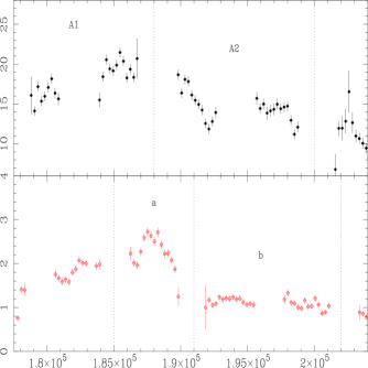
Figure 8: RXTE (top) and ASCA (bottom) light curves corresponding to the most prominent ASCA flare. Intervals a and b in bottom panel correspond to the flare and post-flare phases discussed in Iwasawa et al. (1999).

Figure 9: RXTE light curve depicting the intervals of interest preceding and following the most prominent flare a seen by ASCA .

Figure 10: RXTE light curve depicting the intervals of interest preceding and following the most prominent flare seen by ASCA .

4.3.2 The RXTE flare

We next investigate the time intervals surrounding the RXTE flare (Fig. 11); due unfortunately to an absence of ASCA data during this time interval, we cannot make analogous comparisons. However, we find that changes to the intrinsic power law slope during these intervals follow similar trends presented for the RXTE counterpart of the ASCA flare in the previous section, although events surrounding this bright RXTE flare event appear to be much more erratic and complicated. (We remind the reader that this is also apparent in hardness ratio comparisons during this time interval.) The similarities with the ASCA flare lie in observed trends to changes in $\Gamma_{3-10}$. In particular, there is a noticeable flattening of $\Gamma_{3-10}$ in the transition between ‘ pre- ’ and ‘ post- ’ flare states X1 to X2, which continues through interval m, before suddenly steepening in the following interval n. Unfortunately, errors are such that again we are unable to make any statements regarding changes to $F_{\rm K\alpha}$ or $\Gamma_{10-20}$. However, we note that $F_{\rm K\alpha}$ is generally high for these time intervals associated with this hard RXTE flare event. Table 6 details these results. As with the ASCA flare, Fig. 12 for the RXTE flare hints at changes in $F_{\rm K\alpha}$ on short time intervals (e.g. X1 and m)

Figure 11: RXTE light curve depicting the intervals of interest preceding and following the most prominent flare seen by RXTE .

Figure 12: RXTE light curve depicting the intervals of interest preceding and following the most prominent flare seen by RXTE .

Change in $\Gamma$ for time periods previous to and following RXTE flare
Interval	$\rm\Gamma_{3-10}^{a}$	$E_{\rm K\alpha}^{b}$	$F_{\rm K\alpha}^{c}$	$\rm\Gamma_{10-20}^{d}$	$W_{\rm K\alpha}^{e}$ (eV)	$\rm Flux^{f}$
v	$1.97\pm 0.03$	$6.47\pm 0.14$	$2.13\pm 0.37$	$1.74^{+0.22}_{-0.21}$	$361\pm 63$	4.65
X1	$2.05\pm 0.03$	$6.40\pm 0.12$	$2.50\pm 0.38$	$1.73^{+0.19}_{-0.18}$	$357\pm 54$	5.46
X2	$1.93\pm 0.03$	$6.35\pm 0.10$	$2.19\pm 0.30$	$1.69^{+0.19}_{-0.18}$	$409\pm 57$	4.09
m	$1.83\pm 0.03$	$6.49\pm 0.10$	$1.94\pm 0.24$	$1.57^{+0.16}_{-0.17}$	$457\pm 56$	3.35
n	$1.98\pm 0.03$	$6.46\pm 0.11$	$2.22\pm 0.30$	$1.83^{+0.24}_{-0.23}$	$497\pm 68$	3.58
p	$1.94\pm 0.02$	$6.45\pm 0.07$	$2.48\pm 0.22$	$1.61^{+0.14}_{-0.14}$	$501\pm 45$	3.96

Table 6: Results are quoted from simple power law fits; the diskline model of Fabian et al. (1989) is used to model the line emission. ^a Power-law photon index for 3 keV $<$ E $<$ 10 keV. ^b Centroid energy of iron K$\alpha$ line. ^c Flux of iron emission line in units of $10^{-4}$ ${\rm\thinspace ph}{\rm\thinspace cm}^{-2}{\rm\thinspace s}^{-1}\,$. ^d Power-law photon index for 10 keV $<$ E $<$ 20 keV. ^e Equivalent width of the iron emission line. ^f 3-10 keV flux in units of $10^{-11}$ ${\rm\thinspace erg}{\rm\thinspace cm}^{-2}{\rm\thinspace s}^{-1}\,$.

4.4 The intervals i1 to i7

It is clear from the spectral analysis thus far that conditions can alter suddenly and erratically. In order to assess whether a more simplified picture exists, we investigate spectral features of the deep minima in contrast with flare type events, using a model that consist of simple power law and redshifted Gaussian component. Table 8 confirms the findings of Section 4.2.1 such that in general, $\Gamma_{3-10}$ tends to be flatter during the minima in contrast to the flare states. A close comparison of $\Gamma_{3-10}$ versus $\Gamma_{10-20}$ for the differing states suggests that we are largely seeing intrinsic changes in the power law slope rather than reflection, although it is likely that we are seeing contributions from both effects. Additionally, ratio plots of data against model using a power law fit show that there is a noticeable change in the line flux, profile, as well as the reflection component, similar to that seen in Fig. 7a.

Interval	Exposure	2-60 keV	Time range
	$\rm 10^{3}$ s	$\rm ct$ $\rm s^{-1}$	$\rm 10^{4}s$
i1	6.74	9.59 $\pm$ 0.12	3.0-4.8
i2	9.52	15.86 $\pm$ 0.10	6.0-8.0
i5	5.50	15.78 $\pm$ 0.14	51.0-53.5
i6	17.65	10.50 $\pm$ 0.07	54.0-58.0
i7	19.95	16.47 $\pm$ 0.07	62.0-66.0

Table 7: i1-i7 correspond to the nine intervals of interest for the light curve given in Fig. 1. The intervals i1 and i6 correspond to the deep minima, whereas i2, i5, and i7 have comparable fluxes. Count rates for the intervals are given for the 2-60 keV energy band of the RXTE PCA.

Change in $\Gamma$ for different states of MCG$-$6-30-15
Interval	$\rm\Gamma_{3-10}^{a}$	$F_{\rm K\alpha}^{b}$	$\rm\Gamma_{10-20}^{c}$	$\rm W^{d}$ (eV)	$\rm Flux^{e}$
i1	1.80 $\pm$ 0.06	$1.79^{+0.59}_{-0.45}$	1.77 $\pm$ 0.30	$539^{+178}_{-136}$	2.47
i2	1.97 $\pm$ 0.03	$1.73^{+0.35}_{-0.29}$	1.59 $\pm$ 0.19	$322^{+65}_{-54}$	3.98
i5	1.94 $\pm$ 0.03	$1.91^{+0.62}_{-0.47}$	1.58 $\pm$ 0.16	$318^{+103}_{-78}$	4.17
i6	1.82 $\pm$ 0.03	$1.85^{+0.32}_{-0.28}$	1.56 $\pm$ 0.16	$494^{+85}_{-75}$	2.68
i7	1.98 $\pm$ 0.02	$1.98^{+0.36}_{-0.32}$	1.83 $\pm$ 0.14	$305^{+56}_{-59}$	4.33

Table 8: Results are quoted from simple power law fits; a redshifted Gaussian is used to model the line emission. ^a Power-law photon index for 3 keV $<$ E $<$ 10 keV. ^b Flux of iron emission line in units of $10^{-4}$ ${\rm\thinspace ph}{\rm\thinspace cm}^{-2}{\rm\thinspace s}^{-1}\,$. ^c Power-law photon index for 10 keV $<$ E $<$ 20 keV. ^d Equivalent width of the iron emission line. ^e 3-10 keV flux in units of $10^{-11}$ ${\rm\thinspace erg}{\rm\thinspace cm}^{-2}{\rm\thinspace s}^{-1}\,$.

4.5 Summary of spectral findings

We find evidence from flux-correlated studies that $\Gamma_{3-10}$ steepens significantly with flux ($\rm\Delta\Gamma_{3-10}\sim 0.06$ for a doubling of the flux from f1 to f4; Fig. 13a) while surprisingly, the iron line strength appears to remain constant (at most differing by $\sim 1.5\times 10^{-5}$ ${\rm\thinspace ph}{\rm\thinspace cm}^{-2}{\rm\thinspace s}^{-1}\,$from flux-correlated studies). Changes to $\Gamma_{10-20}$ ($\rm\Delta\Gamma_{10-20}\sim 0.3$) and $W_{\rm K\alpha}$ ($\Delta W_{\rm K\alpha}\sim 200$ eV) are also evident and anticorrelate with flux (Fig. 13b for the latter).

A close look at events corresponding to deep minima versus flares reinforces the finding that changes to the intrinsic power law slope are evident, with a comparably steeper $\Gamma_{3-10}$ value during the flares. Figs. 13 illustrate that the behaviour of the intrinsic photon index and $W_{\rm K\alpha}$ during the flares is consistent with the flux-correlated behaviour.

We find that reflection increases with flux when fitting flux-separated data with a complex model that includes the reflected spectrum. Curiously, reflection fraction $R$ anticorrelates with $W_{\rm K\alpha}$; similarly the absolutely normalization of the reflection component ($Rnorm$) anticorrelates with $F_{\rm K\alpha}$. We note that contrary to findings from simple power law fits, $F_{\rm K\alpha}$ is seen to decrease with flux, when non-unity abundances are assumed. We caution however about the large degeneracies associated with complex fits when only the 3$-$20 keV RXTE data are considered. (The case for requiring supersolar abundances is discussed in Lee et al. 1999). With the exception of the behaviour of $F_{\rm K\alpha}$, all other parameters as e.g. $\Gamma$ display similar trends using complex and simple power law fits. The apparent discrepancy between $F_{\rm K\alpha}$ from simple and complex fits in conjunction with the large errors associated with $F_{\rm K\alpha}$ would suggest that an ambiguity exists in measurements of the iron line itself, which RXTE is unable to resolve.

     

Figure 13: 2$-$10 keV flux versus (a) $\rm\Gamma_{3-10}$, and (b) equivalent width $W_{\rm K\alpha}$. Filled circles represent the different flux states; filled squares and dashed lines represent the ASCA flare intervals; triangles and dot-dashed lines represent RXTE flare intervals.

A detailed investigation of the time intervals surrounding the bright ASCA and RXTE flare reveal further complexities. While changes to $\Gamma_{3-10}$ are consistent with flux-correlated studies, we find that there is evidence to suggest that a change in $F_{\rm K\alpha}$ occurs during the time intervals immediately associated with the flare event; in other words, tentative evidence for changes to $F_{\rm K\alpha}$ are apparent on short time scales. In particular, a large increase in the line flux (e.g A2) is evident in the interval immediately following the flare; $W_{\rm K\alpha}$ increases similarly. It is curious that $F_{\rm K\alpha}$ shows a significant increase after the flare rather than during, and may be an indication that are we witnessing some type of response to the flare (e.g. Fig. 10), but also caution that the evidence is very tentative. We note also that $F_{\rm K\alpha}$ is comparably high ($\sim$ factor of 1.7 increase) during the times surrounding the RXTE flare, and times following the ASCA flare, in contrast to values presented in Tables 2, 3, and 8.

5 Time Lags, Leads, and Reverberation

Motivated by the temporal findings of e.g. Miyamoto et al. (1988) and Cui et al. (1997) for Cygnus X-1, we next wish to investigate whether the collecting area of RXTE coupled with this long observation is sufficient to discern time lags, time leads, and in particular whether reverberation effects can finally be seen. We acknowledge that a good assessment can be hampered by unevenly sampled data, the nature of which has been investigated by a number of workers (e.g. Edelson & Krolik 1998; Yaqoob et al. 1997) for AGN to In‘t Zand & Fenimore (1996) for application to gamma-ray bursts. We adopt a method similar to that presented by Edelson & Krolik (1998). Accordingly, we define the following formalism for our calculations of the autocorrelation function (ACF), and cross correlation function (CCF).

$$CCF(\tau_{i})=\frac{1}{M}\sum_{\it i=-n}^{\it n}\frac{y^{\prime}({\it i}){\it z^{\prime}}({\it i+\tau})}{n_{\tau}}\qquad\mbox{for }\qquad\tau\neq 0$$ (4)

$$\qquad\mbox{where }\qquad z^{\prime}=z_{i}-\frac{\sum_{\it i=1}^{\it n}z_{i}}{n}$$

$$\qquad\mbox{and }\qquad CCF(\tau_{0})=\sum_{\it i=1}^{\it n}(y_{i}-\bar{y})(z_{i}-\bar{z})=M$$

The time interval $\tau$ is incremented by n multiples of 64s ($\tau=n\times 64$); the subsequent definition of $n_{\tau}$ is the number of bins for which the difference in time between consecutive time intervals satisfy the present value for $\tau$. The variables $K$ and $M$ correspond respectively to the ACF and CCF value at $\tau=0$; these terms are used in order to normalize the ACF and CCF so that coherent noise addition at $\tau=0$ is eliminated.

In order to better understand the nature of our findings shown in Figs. 15-17, we run our CCF algorithm on simulated light curves. The light curves over which the CCFs are evaluated are identical except that one has a specified fraction shifted in phase or time. In principle, time- and phase-shifted light curves are identical at certain Fourier frequencies as for example, for the case in which the power spectrum can be represented by a single sine curve. However, if the light curve is the addition of e.g. several sine curves (more representative of actual physical systems), then a time shift will have the effect of shifting the entire pattern by the specified time interval, whereas a phase shift will shift each individual sine curve along by that phase. The final outcome of the phase-shifted light curve will consist of the additive components of the individual sine curves that have been shifted, i.e. the individual frequencies are added together separately. The CCF of the simulated phase- and time-shifted light curves are shown in Figs. 14; solid lines correspond to the CCF, and dashed lines to the mirror image of this. We point out that the CCFs show subtle differences. For the phase-shifted light curve of Fig. 14a, a constant offset from zero is seen between the CCF and its mirror image (represented by respectively the solid and dashed lines). This is contrasted with the time-shifted light curve in which the CCF and its mirror image become comparable (i.e. there is no persistent offset) at $\sim$ 30 bins (i.e. $\sim$1900s). Simulated light curves are generated using Monte Carlo techniques for the flux, with power inversely proportional to frequency, while times are identical to those in the real data. We note that the similarity between the phase- and time-shifted data between 0 and $\sim$10 bins (i.e. $\sim$ 0-640 s) is due to the fact that only 20 per cent of the light curve has been shifted, with the other 80 per cent of the light curve that remain identical between the phase-shifted and time-shifted simulations.

Assessment of the CCFs between the upper continuum (E3 : 7.5-10 keV) and lower continuum (E1 : 3-4.5 keV) and iron line region (E2 : 5-7 keV) shown in Fig. 15, reveal evidence for a possible phase shift. In a comparison with the CCF of the simulated light curve shown in Fig. 14a, in which an artificial phase lag of $\phi\sim$ 0.6 rad is introduced, we find that a similar trend exists in the actual data. This would suggest that $\sim$ 10-20 per cent of the upper continuum band lags that of the lower energy bands E1 and E2.

We next assess the nature of the (10-20 keV) reflection component with the other lower energy bands. In contrast to the previous findings, the CCFs of the reflection component (E4) with the lower continuum (E1), and iron line region (E2) points at possible time shifts ($\mathrel{\hbox to0.0pt{\lower 3.0pt\hbox{$\sim$}\hss}\raise 2.0pt\hbox{$<$}}$ 1000s) as suggested in Fig. 16. Fig. 14b illustrates that the CCFs of a time shifted light curve is marked by a non-symmetric bodily shift of the CCF, whereas this is not the case of the CCF of a light curve with a phase shift.

Fig. 17 shows that neither a time nor phase shift is seen in a comparison of the iron line region (E2) with the lower continuum (E1), and the reflection component (E4) and upper continuum (E3). CCFs of the individual energy bands with itself for all energy bands mentioned thus far look nearly identical to Figs. 17.

We note that errors are such that we are unable to make definitive statements either about a phase or time lag at this time.

     

Figure 14: (a) CCF of simulated light curve with a 20 per cent phase shift of $\sim$ 0.6 radians (solid lines); dashed lines represent the mirror image to this. (b) CCF of simulated light curve with a 20 per cent time shift of 1000s (solid lines); dashed lines represent the mirror image to this.

     

Figure 15: Data points indicate possible phase lag in (a) CCF between the E1 (2$-$4.5 keV) and E3 (7.5$-$10 keV) light curves and (b) CCF between the E2 (5$-$7 keV) and E3 (7.5$-$10 keV) light curves; superimposed on each CCF is its mirror image as represented by the solid lines. For both cases, the pattern between the CCF and its mirror image is similar to that of Fig. 14a for the simulated data, when a phase shift of $\phi=0.6$ rad is applied.

     

Figure 16: Data points indicate possible time lag in (a) CCF between the E1 (2$-$4.5 keV) and E4 (10$-$20 keV) light curves and (b) CCF between the E2 (5$-$7 keV) and E4 (10$-$20 keV) light curves; superimposed on each CCF is its mirror image as represented by the solid lines. For both cases, the pattern between the CCF and its mirror image is similar to that of Fig. 14b for the simulated data, when a time shift of $\mathrel{\hbox to0.0pt{\lower 3.0pt\hbox{$\sim$}\hss}\raise 2.0pt\hbox{$<$}}$ 1000s is applied.

     

Figure 17: There are no indications for obvious shifts, either in phase or time for the CCF of the (a) E1 (2$-$4.5 keV) and E2 (5$-$7 keV) light curves, and (b) the E3 (7.5$-$10 keV) and E4 (10$-$20 keV) light curves.

5.1 Large scale bumps versus small scale flicker

It is interesting to compare our time-lag results with those of Nowak & Chiang (1999) and Reynolds (1999). Nowak & Chiang use similar cross-correlation techniques to those employed here to search for time lags between the soft band (0.5–1.0 keV) ASCA light curve and the hard band (8–15 keV) RXTE light curve. They found that the hard band lags the soft band by $1.6\pm 0.5$ ksec. In this work, we find lags $\mathrel{\hbox to0.0pt{\lower 3.0pt\hbox{$\sim$}\hss}\raise 2.0pt\hbox{$<$}}1000$ s between RXTE bands E1 (2–4.5 keV) and E4 (10–20 keV). Noting that thermal Comptonization predicts a time lag that varies logarithmically with energy, our results are consistent with those of Nowak & Chiang.

Reynolds (1999) uses an interpolation method to constrain trial transfer functions linking two given bands. He found a lag of 50–100 s between the 2–4 keV and 8–15 keV RXTE bands, rather smaller than that found here. To reconcile these results, one must appreciate that these methods probe lags at different Fourier frequencies. The CCF methods tend to probe lags across a broad spectrum of Fourier frequencies. Due to the red nature of the power spectrum, such methods are naturally biased towards the lower Fourier frequencies. The method of Reynolds (1999), instead, probes the higher Fourier frequencies since he uses fairly spiky trial transfer functions. Hence, to paraphrase these technical results, the rapid flickering seems to get transmitted up the observed energy spectrum with a smaller time lag (by an order of magnitude) than experienced by the slower variations.

6 Power spectra and periodicity ?

While spectral studies of X-ray variability in time sequence may hold the key to understanding the underlying processes that are responsible for producing the observed dramatic flux changes, it is insufficient for constraining the size of the emitting region in the absence of a good understanding of the flare mechanisms. The line profile obtained from ASCA observations suggest that the X-ray emission originates from $\sim$ 10-20 gravitational radii of the black hole. This together with a periodic signal can constrain the size of the emitting region. Alternatively, we can attempt to estimate the black hole mass by assessing where the break frequency in the PDS occurs (assuming that the break frequency scales with mass).

We calculate the power density spectrum using the Lomb-Scargle method (Lomb 1976; Scargle 1982; Press et al. 1992) appropriate for unevenly sampled data, and fit a power law slope independently to the RXTE and ASCA data between $10^{-5}$ and $10^{-4}$ Hz. (We ignore data above the latter in order to avoid contamination to the fit from the 96 minute orbital period of RXTE .) Figs. 18 show that respectively, $f^{-1.3}$ and $f^{-1.5}$ is sufficiently representative of the RXTE and ASCA data down to $\sim$ $4-5\times 10^{-6}$ Hz, where the break in the power spectrum may occur. (We note that this value is only given as a limit to $f_{br}$ - while there appears to be no additional evidence for a break below $4-5\times 10^{-6}$ Hz, the observations are insufficiently long to claim a definitive determination.) This is consistent with the findings of Hayashida et al. (1998) for MCG$-$6-30-15. Since the count rate throughout these observations remain steadily between 6-24 ct $\rm s^{-1}$ for RXTE and 0.5-3 ct $\rm s^{-1}$ for ASCA , the findings above would suggest that large scale power does not exist in abundance even though much shorter time scale variability is highly evident.

We note that Papadakis & Lawrence (1993) caution against standard Fourier analysis techniques for estimating power spectra, in the form of a bias of the periodogram due to a windowing effect, in addition to a possible ‘red noise leak’. The former is tied to a concern that the sampling window function can alias power from frequencies above and below the central frequency $\omega_{p}$, thereby distorting the true shape of the power spectrum; the latter ‘red noise leak’ effect is concerned with a transfer of power from low to high frequencies. (The problem of the ‘red noise leak’ was first noted by Deeter & Boyton (1982) and Deeter (1984).) However, we conclude according to subsequent equations (6) and (7) that the effects of this bias is negligible for the data sets in question. The expected value of the periodogram is defined such that :

$$E[I(\omega_{p})]=\int^{\frac{\pi}{\Delta T}}_{-\frac{\pi}{\Delta T}}f(\omega)F_{N}(\omega-\omega_{p})d\omega$$ (5)

where $F_{N}(\omega-\omega_{p})$ is the Fejer kernel (Priestley 1981) which assumes the shape of the $sine^{2}$ function for frequencies $\sim\omega_{p}$. It follows that the bias is :

$$b(\omega)=E[I(\omega_{p})]-f(\omega)$$ (6)

For lengthy time series (e.g. 400 ks), the mean value of the periodogram would tend increasingly more towards the true value of the power spectrum at frequency $\omega_{p}$, as the Fejer kernel becomes increasingly concentrated around this frequency. In any case, we only wish to note that a potential break is seen in the power spectrum at $4-5\times 10^{-6}$ Hz. (A similar break is noted in this object from Ginga data by Hayashida et al. 1998.)

     

Figure 18: Lomb power as function of frequency for (a) RXTE 2-60 keV PCA energy band and (b) ASCA 0.6-10 keV. A power law model was used to fit the data; best fit values for the slope are labeled in the figures.

We wish additionally to point out an interesting possibility for a 33hr periodicity. This is illustrated in Fig. 19 with 33hr interval tickmarks superimposed upon the ASCA and RXTE light curves. This has been determined by taking the mean of the times of the 2 brightest flares in the RXTE light curve (the peak of the RXTE flare X1 and i5, shown in Fig. 1). We note that the power of these peaks is not sufficient to be significant in Lomb-Scargle power spectra (i.e. the sharp peaks do not carry very much power). Accordingly, we have not attempted to quantify the significance of the peaks, and in part also because of the red noise nature of the PDS. We merely point out that 5 out of the 6 tickmarks in the RXTE light curve with flux $\rm>14\thinspace ct\thinspace s^{-1}$ occur in 33 hr intervals, with the same trend seen in the ASCA light curve.

Figure 19: RXTE (upper) and ASCA (lower) lightcurves of MCG$-$6-30-15 from August 1997. Numbering the six tickmarks from left to right, ticks 2 to 5 correspond to small sharp flares seen in the RXTE data; 2, 4 and 5 are also seen in the ASCA data. There is a peak near tick 6 and tick 1 corresponds to the (jagged) exit from a dip. Ticks 2 to 5 are regular to within about 1 per cent.

7 Discussion

There is evidence that the observed spectral variability is complex. However, all evidence points predominantly to a steepening of the spectral index with increasing flux. (Other AGNs that have exhibited spectral variability include NGC7314 Turner 1987; NGC2992 Turner & Pounds 1989; NGC4051 Matsuoka et al. 1990; NGC3227 Turner & Pounds 1989, Pounds et al. 1990; 3C273 Turner et al. 1989, 1990; NGC5548 Nandra et al. 1991, Chiang et al. 1999; NGC4151 Perola et al. 1986, Yaqoob & Warwick 1991;) 1H0419-577 Guainazzi et al. 1998.) This may be indicative of changes in the temperature or optical depth of the Comptonizing medium or of the soft local radiation field. For instance, we can postulate that during periods of intense flux, a substantial amount of the hard X-rays are absorbed by the disk, and thermalized resulting in a source of soft photons. These will pass through the corona and Compton cool it, thereby giving rise to a steeper spectral slope. However, unless we fully understand the nature of the competition between coronal heating and Compton cooling, it is not clear what physics dominates to give the observed behaviour.

The ejection model of Beloborodov (1998) can explain the observed relationship between reflection fraction and spectral index shown in Table 3. In this model, observed spectral features are due to a non static corona, in which flares are accompanied by plasma ejection from the active regions. In other words, the bulk velocity ( $\beta\equiv v/c$ ) in the flare is $>$ 0. As the ‘blobs’ move away (are ejected) from the disk, a decrease in reflection is seen as a result of diminished reprocessing due to special relativistic beaming of the primary continuum radiation away from the disk. The model does not however account for the constancy of the iron line flux.

We note that the possibility that some of the the iron line and reflection may be due to some distant material such as e.g. a torus is ruled out for this data based on (1) I96, and I99 findings for a non-constant, and sometimes absent narrow core seen in long ASCA observations of MCG$-$6-30-15 in 1994 and 1996, and (2) RXTE findings in this paper that the reflection fraction is seen to increase with flux.

7.1 Reflection and the iron line

A major result from the present observations is the enigmatic behaviour of the iron line; the inverse proportionality between $W_{\rm K\alpha}$ and $R$ and of $Rnorm$ with $F_{\rm K\alpha}$. GF91 predict that the bulk of the line arises from fluorescence in optically thick material. In this simple reflection picture, we would expect $R$ and $W_{\rm K\alpha}$ to be proportional to each other provided (1) the Compton reflection continuum does not dominate the iron line region, (2) the state of the illuminated region does not change, and (3) the primary continuum has a fixed spectral shape. We note for the last point that GF91 point out that differences in the photon index up to $\Delta\Gamma\sim 0.2$ (as compared to our flux-correlated findings for $\Delta\Gamma\sim 0.06$) will contribute less than a 10 per cent effect to $W_{\rm K\alpha}$.

This lack of proportionality between $W_{\rm K\alpha}$ and $R$ (and $Rnorm$ with $F_{\rm K\alpha}$), in conjunction with an apparently constant iron line may point at changes to the ionization of the disk in MCG$-$6-30-15, which is explored further below. We note that tentative evidence for observed changes in $F_{\rm K\alpha}$ does exist during time intervals surrounding flare events. Such variability is clear from the ASCA analysis (I99). It is possible that $F_{\rm K\alpha}$ changes on time scales shorter than is resolvable from time-averaged spectra; in other words, changes to $F_{\rm K\alpha}$ may only become resolvable during bright flares.

We note that Chiang et al. (1999) find similar results for the constancy of the iron line and inverse proportionality between $W_{\rm K\alpha}$ and $R$ in their multi-wavelength campaign of the Seyfert 1 galaxy NGC5548.

7.2 A simple model for the observed spectral variations

We propose the following model in order to explain some of the enigmatic properties of the observed variability phenomena. Spectral variability is no doubt complex, and does not conform to the present picture of a cold disk geometry for MCG$-$6-30-15. If however the variable emission from MCG$-$6-30-15 is from a part of the disc which is more ionized, say with an ionization parameter $\xi\sim 100$ (see spectra in Ross & Fabian 1993, Ross et al 1999), then the reflection continuum will respond to the flux while the iron line does so only weakly. At that ionization parameter the iron line can be resonantly scattered by the matter in the surface of the disc and its energy lost to the Auger process (Ross, Fabian & Brandt 1996).

The more highly ionized region could either be the innermost regions of the disc, perhaps within say $6r_{\rm g}$, or the regions directly beneath the most energetic flares. We note that flux-correlated changes in the surface density of the disk can lead to changes to ionization states without incorporating large changes to luminosities (Young et al. 1999, in preparation).

To illustrate in the context of the RXTE light curve shown in Fig. 1, assume that the flux below 10 $\rm ct\thinspace s^{-1}$ reflect physical processes that occur within the radius $6-40r_{g}$. Next, assume that this is enhanced in the $>10\rm\thinspace ct\thinspace s^{-1}$ variability, by flares within $6r_{g}$, where the Auger destruction effect becomes important. Accordingly, this will lead to observable changes in reflection (i.e stronger reflection during the higher flux periods), with minimal changes in $F_{\rm K\alpha}$.

We note that our interpretation that variability largely comes from within the innermost stable orbit for a Schwarzschild black hole may be consistent with the scenario for a very active corona (and hence strong hard X-ray emission) within $6r_{g}$, proposed by Krolik (1999). In this model, magnetic fields within the radius of marginal stability are strong and amplified through shearing of their footpoints, which can enhance variability.

7.3 Implications for Mass Estimates

7.3.1 Constraints from spectral studies

The constancy of the iron line on day-to-day scales suggests that the timescale for variability (i.e. the observed periods for which dramatic flux changes are observed) we are naively probing are much larger (in the ‘standard’ scenario) than the fluorescing region. In other words, slow changes would imply on a naive model much larger crossing times and hence large regions for the crossing times of the continuum. A light-crossing time of the fluorescing region larger than $\sim$ 50 ks (assuming an average radius $\sim 20r_{s}$) will lead to an estimate for the black hole mass $\rm\sim 10^{8}M_{\odot}$. Reynolds (1999) points out however that the bulge/hole mass relationship of Magorrian et al. (1998) implies a much lower mass estimate for MCG$-$6-30-15, by an order of magnitude, of about $\rm\sim 10^{7}M_{\odot}$.

In the scenario of the simple model presented above, and given evidence for short timescale variability of the iron line (here and I99) as well as the location of the flare line found in I99, the constancy of the line suggests that the timescale for variability for which we are probing is much smaller than the fluorescing region and reconciles the above mass problem.

7.3.2 PDS : Analogies with Galactic Black Hole Candidates

Of further interest is the apparent break in the power spectrum of MCG$-$6-30-15 seen in both the RXTE and ASCA data. The origin of the break is not yet known (but see e.g. Edelson & Nandra 1999; Poutanen & Fabian 1999; Kazanas, Hua, & Titarchuk 1997; and Cui et al. 1997 for possible explanations) , but does provide a useful means to determine the black hole mass, through scaling from similar breaks in the power spectrum of the famous galactic black hole candidate (GBH) Cygnus X-1, and other objects like it.

The behaviour of the PDS in MCG$-$6-30-15 is not unlike that of GBHs in the ‘low’ (hard) state (see e.g. Belloni & Hasinger 1990; Miyamoto et al. 1992; van der Klis 1995). Power law slopes (with form $f^{\alpha}$) of order $\alpha\sim\$-1 to -2 are observed at high frequencies and flatten to $\sim 0$ at lower frequencies. If we bridge the gap between AGNs and GBHs and assume that similar physics are at play, we can make predictions for the black hole mass in MCG$-$6-30-15 (using the values for the cutoff frequencies $f_{br}$) by a simple scaling relation with Cygnus X-1. Belloni & Hasinger (1990) report that $f_{br}\sim$ 0.04-0.4 Hz for Cygnus X-1; for MCG$-$6-30-15, we find evidence that $f_{br}\sim 4-5\times 10^{-6}$ Hz. The resulting ratio between the 2 cutoff frequencies is $\sim 10^{4}-10^{5}$. Herrero et al. (1995) argue that the black hole mass in Cygnus X-1 is $\rm\sim 10M_{\odot}$, which leads us to conclude that the mass of the black hole in MCG$-$6-30-15 is $\sim 10^{5}-10^{6}$, smaller than anticipated.

Our mass estimate agrees with that of Hayashida et al. (1998) and Nowak & Chiang (1999) who also used the break frequency and scaling arguments. However, such mass estimates should be treated with extreme caution. The break frequencies in any one given GBHC can vary by one or two orders of magnitude depending upon the exact flux/spectral state of the source. Given that we do not know how to map AGN spectral states into analogous GBHC states, the mass estimate derived above (and that of Nowak & Chiang 1999) will also be uncertain by up to two orders of magnitude. Additionally, it is not entirely clear what timescales to identify the cutoff frequency with. A small black hole mass (i.e. $<$ $\rm 2\times 10^{6}M_{\odot}$) would also imply the presence of a super-Eddington black hole in MCG$-$6-30-15.

7.3.3 A possible 33 hour period

Finally, we address what implications a 33 hr period would have on the black hole mass in MCG$-$6-30-15. If we make the assumption that this is the orbital time scale for e.g. a flare to circumnavigate the black hole in MCG$-$6-30-15, then we can estimate the mass via the relation :

$$M_{BH}(R)=3.1\times 10^{7}\thinspace t_{orb}\thinspace(\frac{R}{10R_{s}})^{-1.5}M_{\odot}$$ (7)

where $R$ is the distance from the center, and $R_{s}\equiv 2r_{g}$ is the Schwarzschild radius (the gravitational radius of the black hole $r_{g}\equiv GM/c^{2}$, and $t_{orb}$ is in days).

The diskline model constrains $R_{in}$ and $R_{out}$ assuming some power law emissivity function ($\propto R^{-\alpha}$) that declines to larger radii. (We note that beyond $r_{out}$ the line emission is negligible.) Accordingly, we expect that most of the power is concentrated in the inner radii. I96 and I99 constrain using time averaged ASCA data $r_{in}\sim(6.7\pm 0.8)r_{g}$ for MCG$-$6-30-15. This combined with $t_{orb}\sim$ 33hr (= 1.375 days) give a mass for the black hole in MCG$-$6-30-15 $\rm\sim 2.6\times 10^{7}\thinspace M_{\odot}$.

8 Conclusion

We summarize below the spectral and timing results of this paper. It is clear that complicated processes are present, the nature of which is not obviously apparent, and may prove to be a challenge to present theoretical models.

$\bullet$ Hardness ratios reveal that spectral variability may be largely attributed to changes in the intrinsic photon index. In particular, spectral hardening is observed during periods of diminished intensity in comparisons of the (7.5$-$10 keV) upper continuum, (5$-$7 keV) iron line region, and (10$-$20 keV) reflection hump with the (3$-$4.5 keV) lower continuum. Particularly hard spectra are noted in a time interval corresponding to $\rm\sim 260~{}ks$ that begins shortly after the hard RXTE flare.

$\bullet$ We find from flux correlated studies that changes to the photon index are evident. In particular, $\Gamma_{3-10}$ steepens while $\Gamma_{10-20}$ flattens with flux; for a doubling of the flux, $\Delta\Gamma_{3-10}\sim 0.06$ and $\Delta\Gamma_{10-20}\sim 0.3$. This coupled with findings for a constant iron line can contribute to the reduced fractional variability in the iron line band noted by Reynolds (1999). We note that changes to $\Gamma_{10-20}$ are significant only with large changes in flux whereas changes in $\Gamma_{3-10}$ are apparent even with subtle changes in flux. This point is well illustrated in detailed studies of the time intervals surrounding the ASCA and RXTE flares. Nevertheless, it would appear that both changes in the intrinsic power law slope (reflected by changes to $\Gamma_{3-10}$), and reflection (reflected by changes to $\Gamma_{10-20}$) both contribute in varying degrees to the overall spectral variability.

$\bullet$ We find curiously that the iron line flux is consistent with being constant over large time intervals on the order of days (but this is not the case on much shorter time intervals of order $\mathrel{\hbox to0.0pt{\lower 3.0pt\hbox{$\sim$}\hss}\raise 2.0pt\hbox{$<$}}$ 12 ks), and the equivalent width anitcorrelates with the continuum flux. (Observed changes to $F_{\rm K\alpha}$ on short time intervals are summarized in the next point.) This may point at evidence for a partially ionized disk.

$\bullet$ From concentrated studies of the time intervals surrounding the RXTE and ASCA flares, we find tentatively that $F_{\rm K\alpha}$ shows a noticeable increase after the flare events. (This is less significant for the periods of the RXTE flare.) This may be an indication that we are witnessing some type of response to the flare. We note that $F_{\rm K\alpha}$ is comparably high ($\sim$ factor of 1.7 larger) during the times surrounding the RXTE flare, and times following the ASCA flare, in contrast to time averaged analysis of flux-correlated data.

$\bullet$ We find tentative evidence from cross correlation techniques for a possible phase lag comparable to $\phi\sim 0.6$ between the (7.5$-$10 keV) upper continuum, and (5$-$7 keV) iron line band and (3$-$4.5 keV) lower continuum.

$\bullet$ CCFs further reveal possible time lags (time delays $\mathrel{\hbox to0.0pt{\lower 3.0pt\hbox{$\sim$}\hss}\raise 2.0pt\hbox{$<$}}$ 1 ks) between the (10$-$20 keV) reflection hump and iron line band, and reflection hump with lower continuum.

$\bullet$ We report an apparent break (from $f^{0}$ to $\sim$ $f^{-1.5}$) of MCG$-$6-30-15 at $\sim 4-5\times 10^{-6}$ Hz ($\sim 56-70$ hrs) seen by both ASCA and RXTE . Scaling with the mass of the GBH Cygnus X-1 gives a smaller than expected black hole mass of $\rm\sim 10^{5}-10^{6}M_{\odot}$ for MCG$-$6-30-15. However, this is unlikely to be a proper estimate of the mass for the black hole in MCG$-$6-30-15. (A black hole mass $<$ $\rm 2\times 10^{6}M_{\odot}$ would make the black hole in MCG$-$6-30-15 super-Eddington.)

$\bullet$ We report on the possibility for a 33 hr period seen in both the ASCA and RXTE light curves. This combined with a value of $\sim 7r_{g}$ for the inner radius, implies black hole mass $\rm\sim 2.6\times 10^{7}\thinspace M_{\odot}$ for MCG$-$6-30-15.

References

- [] Barr P., Mushotzky R.F., 1986, Nat., 320, 421
- [] Belloni T., Hasinger G. 1990, A&A, 230, 103
- [] Beloborodov A.M., 1998, MNRAS, 297, 739
- [] Chiang J., Reynolds C.S., Blaes O.M., Nowak M.A., Murray N., Madejski G., Marshall H.L., Magdziarz P., 1999, ApJ, submitted
- [] Cui W., Zhang S. N., Focke W., Swank J. H., 1997, ApJ, 484, 383
- [] Cui W., Heindl W. A., Rothschild R. E., Zhang S. N., Jahoda, K., Focke, W., 1997, ApJ, 474, L57
- [] Deeter J.E., 1984, ApJ, 281, 482
- [] Deeter J.E., Boynton P.E., 1982, ApJ, 261, 337
- [] Edelson R.A., Krolik J.H., 1998, ApJ, 333, 646
- [] Edelson R., Nandra K., 1999, ApJ, 514, 682
- [] Fabian A.C., Rees M.J., Stella L., White N.E., 1989, MNRAS, 238,729
- [] George I. M., Fabian A. C., 1991, MNRAS, 249, 352
- [] Guainazzi M., Matt G., Molendi S., Orr A., Fiore F., Grandi P., Matteuzzi A., Mineo T., Perola G. C., Parmar A.N., Piro L., 1999, A&A, 341, L27
- [] Guainazzi M., Comastri A., Stirpe G. M., Brandt W. N., Fiore F., Leighly K. M., Matt G., Molendi S., Puchnarewicz E. M., Piro L., Siemiginowska A., 1998, A&A 339, 327
- [] Guilbert P. W., Rees M. J., 1998, MNRAS, 233, 475
- [] Herrero A., Kudritzki R., Gabler R.P., Vilchez J.M., Gabler A., 1995, A&A, 297, 556
- [] Hayashida K., Miyamoto S., Kitamoto S., Negoro H., 1998, 500, 642
- [1] Iwasawa K., Fabian A.C., Brandt W.N., Kunieda H., Misaki K., Reynolds C.S., Terashima Y., 1998, MNRAS, 295L, 201
- [] Iwasawa K., Fabian A. C., Reynolds C. S., Nandra K., Otani C., Inoue H., Hayashida K., Brandt W. N., Dotani T., Kunieda H., Matsuoka M., Tanaka Y., 1996, MNRAS, 282, 1038
- [] Iwasawa, K. , Fabian A.C., Young A.J., Inoue H., Matsumoto C., 1999 MNRAS, 306L, 191
- [] Kazanas D., Hua, X. M., Titarchuk L., 1997, ApJ, 480, 735
- [] Krolik J.H., 1999, ApJ, 515, L73
- [] Lawrence A., Watson M.G., Pounds K.A., Elvis M., 1987, Nat., 325, 694
- [] Lightman A. P., White T. R., 1988, ApJ., 335, 57
- [] Lomb N.R., 1976, Ap&SS, 39, 447
- [] Lee, J.C., Fabian A.C., Reynolds C.S., Iwasawa K., Brandt W.N., 1998, MNRAS, 300, 583
- [] Lee, J.C., Fabian A.C., Brandt W.N., Reynolds C.S., Iwasawa K., 1999, MNRAS, 310, 973
- [] Magdziarz P., Zdziarski A.A., 1995, MNRAS, 273, 837
- [] Magorrian J., Scott T., Richstone D., Bender R., Bower G., Dressler A., et al., 1998, AJ, 115, 2285
- [] Martocchia A., Matt G., 1996, MNRAS, 282, L53
- [] Matsuoka M., Piro L., Yamauchi M., Murakami T., 1990, 361, 440
- [] Matt G., Perola G.C., Piro L., 1991, A&A, 247, 25
- [] McHardy I., Czerny B., 1987, Nat, 325, 696
- [] McHardy I.M., Papadakis I.E., Uttley P., 1998, in The Active X-ray Sky - Results from BeppoSAX and it RXTE , eds. L. Scarsi, H. Bradt, P. Giommi, F. Fiore, Nuclear Physics B (Proc. Suppl.) vol. 69/1-3, p509
- [] Miyamoto S., Kitamoto S., Iga S., Negoro H., Terada K., 1992, ApJ, 391, L21
- [] Miyamoto S., Kitamoto S., Mitsuda K., Dotani T., 1988, Nat, 336, 450
- [] Nandra K., George I.M., Mushotzky R.F., Turner T.J., Yaqoob T., 1997, MNRAS, 476, 602
- [] Nandra K., Pounds K.A., 1994, MNRAS, 268, 405
- [] Nowak M.A., Chiang J., 1999, ApJ., L-, submitted
- [] Papadakis I.E., Lawrence A., 1993, MNRAS, 261, 612
- [] Papadakis I.E., Lawrence A., 1995, MNRAS, 272, 161
- [] Pounds K.A., Nandra K., Stewart G.C., George I.M., Fabian A.C., 1990, Nat, 344, 132
- [] Poutanen J., Fabian A.C., 1999, 306, L31
- [] Press W., et al. 1992, Numerical Refipes : The Art of Scientific Computing, 2nd ed., Cambridge University Press
- [] Priestley M.B., 1981, Spectral Analysis and Time Series. Academic Press, pp 323, 418
- [] Rees M.J., 1984, A&AR, 22, 471
- [] Reynolds C.S., 1999, ApJ, submitted
- [] Reynolds C.S., Fabian A.C., 1997, 290, L1
- [] Reynolds C.S., Fabian A.C., Nandra K., Inoue H., Kunieda H., Iwasawa K., 1995, MNRAS, 277, 901
- [] Ross R.R., Fabian A.C., 1993, 261, 74
- [] Ross R.R., Fabian A.C., Brandt W.N. 1996, 278, 1082
- [] Ross R.R., Fabian A.C., Young A.J., 1999, 306, 461
- [] Scargle J.D., 1982, ApJ, 263, 835
- [] Tanaka Y., Nandra k., Fabian A. C. , Inoue H., Otani C., Dotani T., Hayashida K., Iwasawa K., Kii T., Kunieda H., Makino F., Matsuoka M., 1995, Nat., 375, 659
- [] van der Klis M., 1995, in X-ray Binaries, ed. W. Lewin, J. van Paradijs, & van E. van den Heuvel, Cambridge University Press, 252
- [] Wandel A., Mushotzky R.F., 1986, ApJ, 306, L61
- [] Yaqoob T., McKernan B., Ptak A., Nandra K., Servemitsos P.J., 1997, ApJ, 490, L25
- [] Young A.J., et al. 1999, in preparation
- [] in ‘t Zand, J.J.M., Fenimore E.E., 1996, ApJ, 464, 622
- [] Zdziarski A.A., Fabian, A.C.; Nandra, K.; Celotti, A.; Rees, M.J.; Done, C.,Coppi, P.S.; Madejski, G.M, 1994, MNRAS, 269, L55