Precession of a Freely Rotating Rigid Body.
Inelastic Relaxation in the Vicinity of Poles.

Abstract

When a solid body is freely rotating at an angular velocity ${\bf\Omega}$, the ellipsoid of constant angular momentum, in the space $\Omega_{1},\;\Omega_{2},\;\Omega_{3}$, has poles corresponding to spinning about the minimal-inertia and maximal-inertia axes. The first pole may be considered stable if we neglect the inner dissipation, but becomes unstable if the dissipation is taken into account. This happens because the bodies dissipate energy when they rotate about any axis different from principal. In the case of an oblate symmetrical body, the angular velocity describes a circular cone about the vector of (conserved) angular momentum. In the course of relaxation, the angle of this cone decreases, so that both the angular velocity and the maximal-inertia axis of the body align along the angular momentum. The generic case of an asymmetric body is far more involved. Even the symmetrical prolate body exhibits a sophisticated behaviour, because an infinitesimally small deviation of the body’s shape from a rotational symmetry (i.e., a small difference between the largest and second largest moments of inertia) yields libration: the precession trajectory is not a circle but an ellipse. In this article we show that often the most effective internal dissipation takes place at twice the frequency of the body’s precession. Applications to precessing asteroids, cosmic-dust alignment, and rotating satellites are discussed.

I Introduction

A complex rotational motion of a free solid body is an evidence of its rotation-axis’ wobbling about the angular momentum. Indeed, a solid body in a long-established regime of free rotation must have its axis of rotation parallel to the angular momentum: this configuration will minimise the kinetic energy, the angular momentum being fixed. The body achieves this minimisation by aligning both its axis of rotation and axis of maximal inertia parallel to the angular momentum. By the end of this relaxation the body comes to steady spinning about its maximal-inertia axis. Any deviation from this regime witnesses either of the influence of the tidal forces, or (in the case of comets) of the result of jetting, or of an impact experienced by the body within its characteristic time of relaxation, or of the entire body being a wobbling fragment of an asteroid disrupted by a collision (Giblin & Farinella 1997 )¹, (Giblin et al 1998)², (Asphaug & Scheeres 1999)³. The contest between the impacts (or the tidal forces, or the cometary jetting) on the one hand, and the relaxation mechanism(s) on the other hand, determines the dynamics of the body rotation.

A study of the rotation of asteroids and comets may thus provide valuable information about their recent history. Several examples of complex motion have already been registered. Among the asteroids, 4179 Toutatis furnishes another example of wobble (Ostro et al 1993)⁴, (Ostro et al 1995)⁵, (Ostro et al 1999)⁶; see also    http://www.eecs.wsu.edu/ hudson/asteroids.html ). Among the comets, P/Halley is certainly an example of such a tumbling object (Sagdeev et al 1989)⁷, (Peale & Lissauer 1989)⁸, (Peale 1991)⁹, (Belton et al 1991 )¹⁰, (Samarasinha & A’Hearn 1995)¹¹. Another example is comet 46/P Wirtanen. ROSETTA mission is supposed to explore this comet soon (Hubert & Schwehm 1991)¹². The spacecraft will be carrying a high-resolution OSIRIS imaging system (Thomas et al 1998)¹³ that, probably, will enable the astronomers not only to see the precession but also to observe its relaxation during the 2.5 years of the spacecraft’s escorting the comet. Our estimates^14,41 show that the angular resolution of the currently available equipment gives to such sort of experiment a good chance of success, provided the experiment includes measurements performed at least half a year apart from one another. An important factor influencing the success or failure of such an experiment is the jetting intensity of the particular comet.

Another field of application for this study is the cosmic-dust alignment: some of the alignment mechanisms are very sensitive to coupling between the angular velocity and angular momentum of the interstellar grains (Lazarian & Draine 1999)¹⁵, (Lazarian & Efroimsky 1999)¹⁶.

The third possible application of the developed formalism could be spin stabilisation of spacecrafts, including spacecrafts with a precession damper (Chinnery and Hall 1995)¹⁷, (Hughes 1986)¹⁸, (Levi 1989)¹⁹. An interest in studies of nonrigid-body dynamics with applications to spacecraft motion emerged after launch of ”Explorer” satellite in 1958. (I am thankful to Vladislav Sidorenko for drawing my attention to this example.) The satellite was a very prolate body with 4 small deformable antennas on it. It had been supposed that it would rotate about its minimal-inertia axis. Instability of this motion was a major surprise for mission experts (Modi 1974)²⁰.

On general grounds, the necessity of relaxation is evident: the system must reduce its

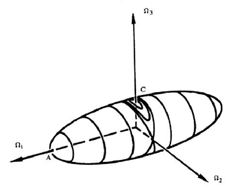
FIG. 1.: The ellipsoid of constant angular momentum in the angular-velocity space ($\Omega_{1}\,,\;\Omega_{2}\,,\;\Omega_{3}$). Lines on its surface denote its intersections with the ellipsoids appropriate to different values of the rotation energy $T_{kin}$. Pole A corresponds to the maximal value of $T_{kin}$ and, thereby, to rotation about the minimal-inertia axis. Pole C corresponds to a complete relaxation, when $T_{kin}$ is minimal and the body is spinning about its major-inertia axis. In the course of precession, the angular-velocity vector $\bf\Omega$ moves along the constant-energy lines, and slowly shifts from one line to another, in the direction from A to C. The above picture describes the case of an almost prolate body: $I_{3}\stackrel{{\scriptstyle>}}{{\sim}}I_{2}>I_{1}$. The trajectories are circular near A and, in this case, remain almost circular all the way from A to the separatrix. Crossing over the separatrix may yield chaotic flipovers, whereafter the body will begin libration. The trajectories will again become circular only in the closemost vicinity of C.

kinetic energy down to the value that is minimal available for a fixed angular momentum. What particular physical effects provide this relaxation? One phenomenon, relevant to tiny grains (like those of the interstellar dust) but feeble for large samples, is the Barnett dissipation called into being by the oscillating (due to the precession) remagnetisation of the material, caused by the Barnett effect. (See, for example, (Lazarian 1994)²¹, (Lazarian & Draine 1997)²², and references therein.) Another process, relevant in small granules, and overwhelmingly leading for large bodies, is the inelastic dissipation. It is produced by the precession-caused alternating stresses and strains.

A pioneering paper on the inelastic dissipation was published by Burns & Safronov²³ back in 1973. Later the inelastic dissipation in small and in large freely-rotating oblate bodies was addressed in (Lazarian & Efroimsky 1999)¹⁶ and (Efroimsky & Lazarian 2000)²⁴, correspondingly. In the present article we shall tackle to the dynamics of a body of arbitrary values of its moments of inertia. The issue is nontrivial. For example, a perfectly biaxial prolate spheroid has two axes of equal maximum moment of inertia and, therefore, really does not have a stable rotation pole. For a triaxial figure of a shape slightly deviating from a symmetrical prolateness, the situation is that the precession trajectory is not a circle but an elongated ellipse, with long axis around the ”waist” of the ”cigar” figure (Fig.1). For the tumbling case, the spin axis circulates all the way around the body, and in fact the circulation is more or less around the long axis. This leads to the curious effect, observed in computer simulations of the rotation of asteroid (433) Eros, that the body appears much of the time to be spinning nearly about its long axis (Black, Nicholson, Bottke, Burns $\&$ Harris 1999)²⁵.

In what follows we briefly review the main facts and formulae describing the solid-body rotation (section II), dwelling comprehensively upon the case of an almost symmetrical prolate body (section III). We divide the motion into four distinct stages (section IV). Then we discuss the relaxation rate (section V) and explain the nature of the nonlinearity emerging in this problem (section VI), whereafter we compute the stresses arising in a precessing body, and calculate the energy density of the appropriate deformations (section VII). In sections VIII and IX we calculate the rate of internal dissipation. In section X we draw conclusions and mention some practical applications of the formalism developed. In section  XI we briefly account of the vississitudes of the generic case.

II Notations and Assumptions

We shall discuss free rotation of a solid body, using two Cartesian coordinate systems, each with an origin at the centre of mass of the body. The inertial coordinate system ($X$, $Y$, $Z$), with unit vectors ${\mathbf{e}}_{X}$, ${\mathbf{e}}_{Y}$, ${\mathbf{e}}_{Z}$, will have its $Z$ axis parallel to the (conserved) angular momentum $\mathbf{J}$. Coordinates with respect to this frame are denoted by the same capital letters: $X$, $Y$, and $Z$. We shall also use the body frame defined by the three principal axes of inertia: $1$, $2$, and $3$, with coordinates $x$, $y$, $z$ and unit vectors $\mathbf{e}$₁, $\mathbf{e}$₂, $\mathbf{e}$₃.

We denote the angular velocity by $\bf{\Omega}$, while $\bf{\omega}$ will stand for the rate of precession. Components of $\bf{\Omega}$ in the body frame will be called $\;\Omega_{1,2,3}\;$.

Due to the lack of an established convention on notations, we present a table that hopefully will prevent misunderstandings.

	Principal moments	Components of angular	Frequency of
	of inertia	velocity	precession
(Purcell 1979),
(Lazarian &
Efroimsky 1999),
(Efroimsky 2000),
(Efroimsky &	$I_{3}\;\geq\;I_{2}\;\geq\;I_{1}$	$\Omega_{3}\;\;,\;\;\;\Omega_{2}\;\;,\;\;\;\Omega_{1}$	$\omega$
Lazarian 2000),
present article
(Synge & Griffiths 1959)	$A\geq B\geq C$	$\omega_{1}\;\;,\;\;\;\omega_{2}\;\;,\;\;\;\omega_{3}$	$p$
(Black et al. 1999)	$C\geq B\geq A$	$\omega_{c}\;\;,\;\;\;\omega_{b}\;\;,\;\;\;\omega_{a}$	$\nu$

A free rotation of a body obeys the Euler equations

$$\frac{d}{dt}\;\left(I_{i}\;\Omega_{i}\right)\;=\;\left(I_{j}\;-\;I_{k}\right)\;\Omega_{j}\;\Omega_{k}$$ (1)

where $\;(i,j,k)\;=\;(1,2,3)\;$ (with cyclic transpositions), and the principal moments of inertia are assumed to obey:

$$I_{1}\;\leq\;I_{2}\;\leq\;I_{3}\;\;\;\;.$$ (2)

In the approximation of an absolutely solid body, the equations simplify:

$$I_{i}\;{\dot{\Omega}}_{i}\;=\;\left(I_{j}\;-\;I_{k}\right)\;\Omega_{j}\;\Omega_{k}\;\;\;\;.$$ (3)

This neglect of $\;{\dot{I}}_{i}\,\Omega_{i}\;$ against $\;I_{i}\;{\dot{\Omega}}_{i}\;$ does need a justification, because the inelastic relaxation we are going to describe is due to small deformations that yield nonzero $\;\dot{I_{i}}\;$. To validate the neglection, i.e., to prove that $\;\dot{I_{i}}/{I_{i}}\;\ll\;\dot{\Omega_{i}}/{\Omega_{i}}\;$, one must recall that for a rotational period $\tau$

$${\dot{\Omega}}_{i}/{\Omega}_{i}\;\approx\;{\tau}^{-1}\;\;\;,\;\;\;\;\;{\dot{I}}_{i}/{I}_{i}\;\approx\;{\tau}^{-1}\,\epsilon\;\;\;$$ (4)

$\epsilon$ being a typical value of the relative strain (which in real life rarely exceeds $10^{-6}$).

Conservation of the angular momentum $\;\bf{J}\;$ and the kinetic energy $\;T_{kin}\;$ entails:

$$I_{1}^{2}\,{\Omega}_{1}^{2}\;+\;I_{2}^{2}\,{\Omega}_{2}^{2}\;+\;I_{3}^{2}\,{\Omega}_{3}^{2}\;=\;{\bf{J}}^{2}\;\;\;,$$ (5)

$$I_{1}\,{\Omega}_{1}^{2}\;+\;I_{2}\,{\Omega}_{2}^{2}\;+\;I_{3}\,{\Omega}_{3}^{2}\;=\;2\;T_{{kin}}$$ (6)

In the context of our study (which is aimed at estimating the rate of relaxation), equation (6) is applicable as long as we accept the adiabatic approach, i.e., assume the relaxation to be a ”slow process”, compared to the ”fast processes” of rotation and precession. A rigorous formulation of this assertion is based on formulae (173) and (270) obtained below. These formulae are to become the main result of our article. They give the relaxation rate $\;d{<\sin^{2}\theta>}/dt\;$, $\;\theta\;$ being the angle between the angular momentum and the major-inertia axis of the body, and averaging being performed over the precession period (Appendix A, formula (A1)). The exact formulation of the adiabatic approach will read:

$$-\;\frac{d\,<\sin^{2}\theta>}{dt}\,\ll\,\omega\;\;,$$ (7)

$\omega\;$ being the precession rate. This condition will adumbrate the applicability realm of the solutions (173) and (270) to be derived.

Equations (5) and (6) may be resolved with respect to $\;{\Omega}_{1}^{2}\;$ and $\;{\Omega}_{2}^{2}\;$:

$${\Omega}_{3}^{2}\;=\;P\;-\;Q\,{\Omega}_{2}^{2}\;\;\;\;,\;\;\;\;\;\;P\;\equiv\;\frac{2\,I_{1}\,T_{kin}\;-\;{\bf J}^{2}}{I_{3}\,(I_{1}\,-\,I_{3})}\;\;\;\;,\;\;\;\;\;\;\;\;Q\;\equiv\;\frac{I_{2}}{I_{3}}\;\frac{I_{1}\,-\,I_{2}}{I_{1}\,-\,I_{3}}\;\;\;\;\;\;\;\;$$ (8)

(9)

$${\Omega}_{1}^{2}\;=\;R\;-\;S\,{\Omega}_{2}^{2}\;\;\;\;,\;\;\;\;\;\;R\;\equiv\;\frac{2\,I_{3}\,T_{kin}\,-\,{\bf J}^{2}}{I_{1}\,(I_{3}\,-\,I_{1})}\;\;\;\;,\;\;\;\;\;\;\;\;S\,\equiv\,\frac{I_{2}}{I_{1}}\,\frac{I_{3}\,-\,I_{2}}{I_{3}\,-\,I_{1}}\,\;\;\;\;\;\;\;\;$$ (10)

substitution whereof in (3), for $\;{\mathit{i}}=2\;$, gives:

$${\dot{\Omega}}_{2}^{2}\;=\;\left(\frac{I_{3}\;-\;I_{1}}{I_{2}}\right)^{2}\;\left(P\;-\;Q\,{\Omega}_{2}^{2}\right)\;\left(R\;-\;S\,{\Omega}_{2}^{2}\right)\;\;\;\;.$$ (11)

It is possible (Synge & Griffith 1959)²⁶ to pick up such positive functions $\;\beta\;$, $\;\omega\;$, $\;k\;$ of the arguments $\;I_{1,2,3},\;T_{kin},\;{\bf{J}}^{2}\;$ that the rescaled time and second component of the angular velocity,

$$t^{\prime}\;\equiv\;\omega\,t\;\;\;,\;\;\;\;\xi\;\equiv\;\Omega_{2}/\beta\;\;\;\;,$$ (12)

satisfy

$$\left(d\xi/dt^{\prime}\right)^{2}\;=\;\left(1\;-\;\xi^{2}\right)\left(1\;-\;k^{2}\;\xi^{2}\right)$$ (13)

with $\;k\;<\;1\;$. Solution to this equation is the Jacobian elliptic function $\;{\textit{sn}}{(t^{\prime})}\;$, so that

$$\Omega_{2}\;=\;\beta\,\;sn\left[\omega(t\,-\,t_{0}),\;k^{2}\right]$$ (14)

$t_{o}$ being an arbitrary constant. It is known (Ibid.) that substitution of the latter in (9) yields, for $\;\;{\bf{J}}^{2}\;>\;2\;I_{2}\;T_{{kin}}\;$ :

$$\Omega_{1}\;=\;\gamma\;\,{\it{cn}}\left[\omega(t\,-\,t_{0}),\;k^{2}\right]\;\;\;,\;\;\;\;\;\;\Omega_{3}\;=\;\alpha\;\,{\it{dn}}\left[\omega(t\,-\,t_{0}),\;k^{2}\right]$$ (15)

(Recall that what we call $\;{\Omega_{3}}\;$, in (Synge & Griffiths)²⁶ is called ${\omega_{1}}$, while (Black et al)²⁵ denote it $\;{{\omega}_{c}}$.) In the above formulae

(16)

$$\alpha\;=\;\sqrt{\frac{{\bf{J}}^{2}\;-\;2\;I_{1}\;T_{{kin}}}{I_{3}\;(I_{3}-I_{1})}}\;\;\;,\;\;\;\;\beta\;=\;\sqrt{\frac{2\;I_{3}\;T_{{kin}}\;-\;{\bf{J}}^{2}}{I_{2}\;(I_{3}-I_{2})}}\;\;\;,\;\;\;\;\gamma\;=\;\sqrt{\frac{2\;I_{3}\;T_{{kin}}\;-\;{\bf{J}}^{2}}{I_{1}\;(I_{3}-I_{1})}}$$ (17)

$$\omega\;=\;\sqrt{\frac{\left({\bf{J}}^{2}\;-\;2\;I_{1}\;T_{{kin}}\right)\;\left(I_{3}\;-\;I_{2}\right)}{I_{1}\;I_{2}\;I_{3}}}\;\;\;,\;\;\;\;k\;=\;\sqrt{\frac{I_{2}\;-\;I_{1}}{I_{3}\;-\;I_{2}}\;\;\frac{2\;I_{3}\;T_{{kin}}\;-\;{\bf{J}}^{2}}{{\bf{J}}^{2}\;-\;2\;I_{1}\;T_{{kin}}}}\;\;\;,$$ (18)

while for $\;{\bf{J}}^{2}\;<\;2\;I_{2}\;T_{{kin}}\;$ one arrives to:

$$\Omega_{1}\;=\;\gamma\;\,{\it{dn}}\left[\omega(t\,-\,t_{0}),\;k^{2}\right]\;\;\;,\;\;\;\;\;\;\Omega_{3}\;=\;\alpha\;\,{\it{cn}}\left[\omega(t\,-\,t_{0}),\;k^{2}\right]$$ (19)

where

(20)

$$\alpha\;=\;\sqrt{\frac{{\bf{J}}^{2}\;-\;2\;I_{1}\;T_{{kin}}}{I_{3}\;(I_{3}-I_{1})}}\;\;\;,\;\;\;\;\beta\;=\;\sqrt{\frac{{\bf{J}}^{2}\;-\;2\;I_{1}\;T_{{kin}}}{I_{2}\;(I_{2}-I_{1})}}\;\;\;,\;\;\;\;\gamma\;=\;-\;\sqrt{\frac{2\;I_{3}\;T_{{kin}}\;-\;{\bf{J}}^{2}}{I_{1}\;(I_{3}-I_{1})}}$$ (21)

$$\omega\;=\;\sqrt{\frac{\left(2\;I_{3}\;T_{{kin}}\;-\;{\bf{J}}^{2}\right)\;\left(I_{2}\;-\;I_{1}\right)}{I_{1}\;I_{2}\;I_{3}}}\;\;\;,\;\;\;\;k\;=\;\sqrt{\frac{I_{3}\;-\;I_{2}}{I_{2}\;-\;I_{1}}\;\;\frac{{\bf{J}}^{2}\;-\;2\;I_{1}\;T_{{kin}}}{{2\;I_{3}\;T_{{kin}}\;-\;{\bf{J}}^{2}}}}\;\;\;,$$ (22)

In some books (like for example in Abramovitz & Stegun 1964)²⁷ notation $\,m\,\equiv\,k^{2}\,$ is used

Mind that in ${Synge\;\&\;Griffith}^{26}$ expression (14.116a) for $\gamma$ is given with a wrong sign. Our expression for $\gamma$, as given by our formula (18), makes the expressions (14 - 15) coincide, in the limit of oblate symmetry ($\;I_{1}\;=\;I_{2}\;$), with the well-known Eulerian solution: $\;\Omega_{1}\,=\,\Omega_{\perp}\,\cos\omega(t-t_{0})\;$, $\;\Omega_{2}\,=\,\Omega_{\perp}\,\sin\omega(t-t_{0})\;$, $\;\Omega_{3}\,=\,const\;$, for $\;\Omega_{3}\,>\,0\;$. Our choice of signs is correct since it leaves $\;\bf\Omega\;$ parallel to $\;\bf J\;$ in the relaxation limit.

Our ultimate goal is to compute the rate of inelastic dissipation caused by alternating stresses in a wobbling body. To know the picture of stresses, one should begin with derivation of the acceleration experienced by a point $\;(x,\;y,\;z)\;$ inside the body. We mean, of course, the acceleration with respect to the inertial coordinate system $\;(X,\;Y,\;Z)\;$, but for convenience of the further calculations we shall express it in terms of coordinates $\;(x,\;y,\;z)\;$ of the body frame $\;(1,\;2,\;3)\;$. The position, velocity and acceleration in the inertial frame will be denoted as $\;{\bf{r}},\;{\bf{v}},\;{\bf{a}}\;$, while those relative to the body frame $\;(1,\;2,\;3)\;$ will be called $\;{\bf{r}}^{\prime},\;{\bf{v}}^{\prime}\;$ and $\;{\bf{a}}^{\prime}\;$ (where $\;{\bf{r}}^{\prime}\;=\;{\bf{r}}\;$). The proper acceleration (i.e., that relative to the inertial frame) will read:

$${\bf{a}}\;\;=\;\;{\bf{a}}^{\prime}\;+\;{\bf{{\dot{\Omega}}}}\;\times\;{\bf{r}}^{\prime}\;+\;2\;{\bf{\Omega}}\;\times\;{\bf{v}}^{\prime}\;+\;{\bf{\Omega}}\;\times\;({\bf{\Omega}}\times{\bf{r}}^{\prime})\;\;\;\;.$$ (23)

In the beginning of this section we justified, on the grounds of the strains being small, our neglect of $\;{\dot{I_{j}}}\,{\Omega}\;$ against $\;{I_{j}}\,{\dot{\Omega}}\;$. In a similar manner we shall justify the neglection of the first and third terms in the right-hand side of the above formula: rotation with a period $\;\tau\;$, of a body of size $\;\mathit{l}\;$ will yield deformations $\;\delta{\mathit{l}}\;\approx\;\epsilon\,{\mathit{l}}$ and deformation-caused velocities $\;v^{\prime}\,\approx\,\delta\mathit{l}/\tau\;\approx\;\epsilon\,\mathit{l}/\tau\;$ and accelerations $\;a^{\prime}\,\approx\,\delta\mathit{l}/\tau^{2}\;=\;\epsilon\,\mathit{l}/\tau^{2}\;$, $\;\epsilon\;$ being the relative strain. We see that $\;v^{\prime}\;$ and $\;a^{\prime}\;$ are much less than the velocities and accelerations of the body as a whole (that are about $\;{\mathit{l}}/\tau\;$ and $\;{\mathit{l}}/{\tau}^{2}\;$, correspondingly). Henceforth,

$${\bf{a}}\;\;\approx\;\;{\bf{{\dot{\Omega}}}}\;\times\;{\bf{r}}^{\prime}\;+\;{\bf{\Omega}}\;\times\;({\bf{\Omega}}\times{\bf{r}}^{\prime})\;=$$ (24)

$${{\bf{e}}_{1}}\;\{\;\left[{\dot{\Omega}}_{2}\;z\;-\;{\dot{\Omega}}_{3}\;y\right]\;+\;{\Omega}_{2}\;\left(\Omega_{1}\;y\;-\;\Omega_{2}\;x\right)\;-\;{\Omega}_{3}\;\left(\Omega_{3}\;x\;-\;\Omega_{1}\;z\right)\;\}$$ (25)

$$+\;\;{{\bf{e}}_{2}}\;\{\;\left[{\dot{\Omega}}_{3}\;x\;-\;{\dot{\Omega}}_{1}\;z\right]\;+\;{\Omega}_{3}\;\left(\Omega_{2}\;z\;-\;\Omega_{3}\;y\right)\;-\;{\Omega}_{1}\;\left(\Omega_{1}\;y\;-\;\Omega_{2}\;x\right)\;\}$$ (26)

$$+\;\;{{\bf{e}}_{3}}\;\{\;\left[{\dot{\Omega}}_{1}\;y\;-\;{\dot{\Omega}}_{2}\;x\right]\;+\;{\Omega}_{1}\;\left(\Omega_{3}\;x\;-\;\Omega_{1}\;z\right)\;-\;{\Omega}_{2}\;\left(\Omega_{2}\;z\;-\;\Omega_{3}\;y\right)\;\}\;\;=$$ (27)

(28)

$$=\;\;{{\bf{e}}_{1}}\;\{\;{\dot{\Omega}}_{2}\;z\;-\;{\dot{\Omega}}_{3}\;y\;-\;x\;\left(\Omega_{2}^{2}\;+\;\Omega_{3}^{2}\;\right)\;+\;y\;\Omega_{1}\;\Omega_{2}\;+\;z\;\Omega_{1}\;\Omega_{3}\;\}$$ (29)

$$+\;\;{{\bf{e}}_{2}}\;\{\;{\dot{\Omega}}_{3}\;x\;-\;{\dot{\Omega}}_{1}\;z\;-\;y\;\left(\Omega_{3}^{2}\;+\;\Omega_{1}^{2}\;\right)\;+\;z\;\Omega_{3}\;\Omega_{2}\;+\;x\;\Omega_{1}\;\Omega_{2}\;\}$$ (30)

$$+\;\;{{\bf{e}}_{3}}\;\{\;{\dot{\Omega}}_{1}\;y\;-\;{\dot{\Omega}}_{2}\;x\;-\;z\;\left(\Omega_{1}^{2}\;+\;\Omega_{2}^{2}\;\right)\;+\;x\;\Omega_{1}\;\Omega_{3}\;+\;y\;\Omega_{2}\;\Omega_{3}\;\}\;\;\;.$$ (31)

where, according to (9) and (14):

$$\Omega_{3}^{2}+\Omega_{2}^{2}\;=\;P+(1-Q)\;\beta^{2}\;{\mathit{sn}}^{2}\left[\omega(t-t_{0}),\;k^{2}\right]\;\;\;,$$ (32)

$$\Omega_{1}^{2}+\Omega_{2}^{2}\;=\;R+(1-S)\;\beta^{2}\;{\mathit{sn}}^{2}\left[\omega(t-t_{0}),\;k^{2}\right]\;\;\;,$$ (33)

$$\Omega_{3}^{2}\;+\;\Omega_{1}^{2}\;=\;(P\;+\;R)\;-\;(Q\;+\;S)\;\beta^{2}\;{\mathit{sn}}^{2}\left[\omega(t\;-\;t_{0}),\;k^{2}\right]\;\;,$$ (34)

$$\Omega_{3}\;\Omega_{1}\;=\;\alpha\;\gamma\;\,{\mathit{dn}}\left[\omega(t\;-\;t_{0}),\;k^{2}\right]\;\,{\mathit{cn}}\left[\omega(t\;-\;t_{0}),\;k^{2}\right]\;\;\;\;,$$ (35)

$${\dot{\Omega}}_{2}\;=\;\beta\;\omega\;{\mathit{cn}}\left[\omega(t-t_{0}),\;k^{2}\right]\;\,{\mathit{dn}}\left[\omega(t-t_{0}),\;k^{2}\right]$$ (36)

the derivative being written in compliance with (Abramovitz & Stegun 1964)²⁷, equation 16.16.1. The other items emerging in (31) will read, for $\;{\textbf{J}}^{2}\;>\;2\,I_{2}\,T_{{kin}}\;$:

$$\Omega_{3}\;\Omega_{2}\;=\;\alpha\;\beta\;\,{\mathit{dn}}\left[\omega(t\;-\;t_{0}),\;k^{2}\right]\;\,{\mathit{sn}}\left[\omega(t\;-\;t_{0}),\;k^{2}\right]\;\;\;\;,$$ (37)

$$\Omega_{2}\;\Omega_{1}\;=\;\beta\;\gamma\;\,{\mathit{cn}}\left[\omega(t\;-\;t_{0}),\;k^{2}\right]\;\,{\mathit{sn}}\left[\omega(t\;-\;t_{0}),\;k^{2}\right]\;\;\;\;,$$ (38)

$${\dot{\Omega}}_{1}\;=\;-\;\gamma\;\omega\;{\mathit{sn}}\left[\omega(t-t_{0}),\;k^{2}\right]\;\,{\mathit{dn}}\left[\omega(t-t_{0}),\;k^{2}\right]\;\;\;\;,$$ (39)

and

$${\dot{\Omega}}_{3}\;=\;-\;\alpha\;\omega\;k^{2}\;{\mathit{cn}}\left[\omega(t-t_{0}),\;k^{2}\right]\;\,{\mathit{sn}}\left[\omega(t-t_{0}),\;k^{2}\right]\;\;\;\;,$$ (40)

while for $\;{\textbf{J}}^{2}\;<\;2\,I_{2}\,T_{{kin}}\;$:

$$\Omega_{3}\;\Omega_{2}\;=\;\alpha\;\beta\;\,{\mathit{cn}}\left[\omega(t\;-\;t_{0}),\;k^{2}\right]\;\,{\mathit{sn}}\left[\omega(t\;-\;t_{0}),\;k^{2}\right]\;\;\;\;,$$ (41)

$$\Omega_{2}\;\Omega_{1}\;=\;\beta\;\gamma\;\,{\mathit{dn}}\left[\omega(t\;-\;t_{0}),\;k^{2}\right]\;\,{\mathit{sn}}\left[\omega(t\;-\;t_{0}),\;k^{2}\right]\;\;\;\;,$$ (42)

$${\dot{\Omega}}_{1}\;=\;-\;\gamma\;\omega\;k^{2}\;{\mathit{sn}}\left[\omega(t-t_{0}),\;k^{2}\right]\;\,{\mathit{cn}}\left[\omega(t-t_{0}),\;k^{2}\right]\;\;\;\;,$$ (43)

and

$${\dot{\Omega}}_{3}\;=\;-\;\alpha\;\omega\;{\mathit{sn}}\left[\omega(t-t_{0}),\;k^{2}\right]\;\,{\mathit{dn}}\left[\omega y(t-t_{0}),\;k^{2}\right]$$ (44)

III Almost Prolate Body

Before pursuing the generic case, let us dwell for a minute on the case of an almost symmetric prolate top of $\;I_{3}\;$ and $\;I_{2}\;$ having close values:

$$I_{3}\;\stackrel{{\scriptstyle>}}{{\sim}}\;I_{2}\;>\;I_{1}\;\;\;,$$ (45)

i.e.,

$$I_{3}\;-\;I_{1}\;\stackrel{{\scriptstyle>}}{{\sim}}\;I_{2}\;-\;I_{1}\;\gg\;I_{3}\;-\;I_{2}\;\stackrel{{\scriptstyle>}}{{\sim}}\;0\;\;\;\;.$$ (46)

As we saw above, the solution depends upon the sign of $\;({\textbf{J}}^{2}\;-\;2\,I_{2}\,T_{{kin}})\;$. According to (5 - 6),

$${\textbf{J}}^{2}\;-\;2\,I_{2}\,T_{{kin}}\;=\;\Omega_{3}^{2}\;I_{3}^{2}\;-\;\Omega_{3}^{2}\;I_{3}\;I_{2}\;+\;\Omega_{1}^{2}\;I_{1}^{2}\;-\;\Omega_{1}^{2}\;I_{1}\;I_{2}\;=\;\Omega_{3}^{2}\;I_{3}^{2}\;\left[\frac{I_{3}\;-\;I_{2}}{I_{3}}\;-\;\frac{\Omega_{1}^{2}}{\Omega_{3}^{2}}\;\frac{I_{1}}{I_{3}}\;\frac{I_{2}\;-\;I_{1}}{I_{3}}\right]$$ (47)

Based on (45 - 46), one can introduce the following parameters:

$$q\;\equiv\;\frac{I_{3}\;-\;I_{2}}{I_{3}}\;\;\;\;,$$ (48)

and

$$s\;\equiv\;\frac{I_{1}}{I_{3}}\;\;\;\;.$$ (49)

Besides, we shall use a time-dependent quantity $\;{\Omega_{1}^{2}}/{\Omega_{3}^{2}}\;$. It is not, of course, a geometrical parameter worthy of the name, though formally one may consider it as a sort of parameter in (47). This wanna-be parameter may be used as a measure of the system’s approaching the steady regime: if $\;{\Omega_{1}^{2}}/{\Omega_{3}^{2}}\;\ll\;1\;$ over the entire time of one wobble then the relaxation is almost over, and the angular velocity $\;{\bf{\Omega}}\;$ is precessing about $\;{\bf{J}}\;$, with a small amplitude (i.e., describing a narrow cone). Below, the meaning of the words like small and narrow will become understandable. Meanwhile, one can write down (47) as

$${\textbf{J}}^{2}\;-\;2\;I_{2}\;T_{{kin}}\;=\;\Omega_{3}^{2}\;I_{3}^{2}\;\left[q\;-\;\frac{\Omega_{1}^{2}}{\Omega_{3}^{2}}\;s\;(1\;-\;s\;-\;q\;)\right]\;\;\;\;,$$ (50)

and easily find that for fixed values of $\;q\;$ and $\;s\;$ (i.e., for a particular prolate body) the narrowness of the precession cone yields:

$${\textbf{J}}^{2}\;-\;2\;I_{2}\;T_{{kin}}\;\approx\;\Omega_{3}^{2}\;I_{3}^{2}\;q\;\;\;.$$ (51)

This approximation becomes true at the late stage of relaxation, when

$$\frac{\Omega_{1}^{2}}{\Omega_{3}^{2}}\;\ll\;q\;\frac{1}{s(1-s-q)}$$ (52)

holds through the duration of one wobble. Assume, following (Black, Nicholson, Bottke, Burns $\&$ Harris 1999)²⁵, that the moments of inertia of asteroid (433) Eros relate as $\;\;\;I_{1}\;:\;I_{2}\;:\;I_{3}\;\;=\;\;1\;:\;3\;:\;3.05\;$. With these numbers plugged in, the above formula will give: $\;|\Omega_{1}/\Omega_{3}|\;\ll\;0.4\;$. Formally, (51) was derived from (50) by keeping $\;q\;$ and $\;s\;$ fixed, and making the ”parameter” $\;{\Omega_{1}^{2}}/{\Omega_{3}^{2}}\;$ approach zero. After this is done, one may consider a variety of geometries, and make $\;q\;$ approach zero. Then $\;{\textbf{J}}^{2}\;-\;2\;I_{2}\;T_{{kin}}\;$ will approach zero, always remaining positive, so that the end of relaxation will be described by the solution (14, 15) with frequency $\;\omega\;$ expressed by (18).

On the other hand, one might as well perform a different, unphysical trick: for a fixed $\;\Omega_{1}\;$, begin with a limit $\;q\;\rightarrow\;0\;$, and only afterwards choose the case of the small-amplitude wobble (i.e., consider $\;{\Omega_{1}^{2}}/{\Omega_{3}^{2}}\;\rightarrow\;0\;$). The first limit will give:

$${\textbf{J}}^{2}\;-\;2\;I_{2}\;T_{{kin}}\;\approx\;-\;\Omega_{3}^{2}\;I_{3}^{2}\;\frac{\Omega_{1}^{2}}{\Omega_{3}^{2}}\;s\;(1-s)\;\;\;,$$ (53)

After the second limit is taken, $\;{\textbf{J}}^{2}\;-\;2\;I_{2}\;T_{{kin}}\;$ will approach zero, always remaining negative, so that the final stage of relaxation would obey the solution (14, 19) with frequency $\;\omega\;$ expressed by (22).

We see that the operations $\;q\;\rightarrow\;0\;$ and $\;{\Omega_{1}^{2}}/{\Omega_{3}^{2}}\;\rightarrow\;0\;$ do not commute. From the physical point of view, an observer studying, for a variety of samples, the end of relaxation should first fix the shape of the body (i.e., assume, for example, that $\;q\;$ is small enough but constant). Only afterwards he may state that he is interested only in the final spin, i.e., assume $\;{\Omega_{1}^{2}}/{\Omega_{3}^{2}}\;\ll\;q\;s^{-1}\;(1-s-q)^{-1}\;$. As explained above, this observer will see that the end of relaxation takes place at frequency $\;\omega\;$ expressed by (18).

An opposite order of limits would be physically meaningless, in that it would not help us to describe the behaviour of a particular body.

We had to dwell on this issue so comprehensively because it would be very important to understand better the following two statements made in (Black, Nicholson, Bottke, Burns $\&$ Harris 1999)²⁵:

1). In the limit where $\;I_{1}\;=\;I_{2}\;$, the circulation region around the maximal-inertia axis vanishes, and

2). All trajectories circulate around the minimal-inertia axis. (This statement is fortified by the following argument: “the slightest perturbation would cause such an object to “roll” about its long axis.”)

To analyse this statement by Black, Nicholson, Bottke, Burns $\&$ Harris ²⁵, let us cast it in a more exact form. First of all, we should understand which of the two possible sequencies of limits these authors implied. In case their statement implied the limit $\;q\;\rightarrow\;0\;$ taken first, and the relaxation limit $\;{\Omega_{1}^{2}}/{\Omega_{3}^{2}}\;\rightarrow\;0\;$ taken afterwards, then according to (22) the frequency of precession $\;\omega\;$ will read as

$$\omega\;=\;\sqrt{\frac{\left(2\;I_{3}\;T_{{kin}}\;-\;{\bf{J}}^{2}\right)\;\left(I_{2}\;-\;I_{1}\right)}{I_{1}\;I_{2}\;I_{3}}}\;=\;\sqrt{\frac{\left(\Omega_{2}^{2}\;I_{2}\;(I_{3}\;-\;I_{2})\;+\;\Omega_{1}^{2}\;I_{1}\;(I_{3}\;-\;I_{1})\right)\;\left(I_{2}\;-\;I_{1}\right)}{I_{1}\;I_{2}\;I_{3}}}\;\rightarrow$$ (54)

(55)

$$\rightarrow\;\sqrt{\frac{\left(I_{3}\;-\;I_{1}\right)\;\left(I_{2}\;-\;I_{1}\right)}{I_{2}\;I_{3}}}\;|\Omega_{1}|\;\;\;,\;\;\;for\;\;\;q\;\rightarrow\;0\;\;\;and\;\;\;\Omega_{1}\;\;being\;\;fixed.\;\;\;\;\;\;\;\;\;$$ (56)

It will then approach zero as $\;|\Omega_{1}|\;$. However, as explained above, such a sequence of limits would be unphysical, while a physical way is to fix the body shape first (i.e., to fix the difference $\;(I_{3}\,-\,I_{2})\;$), then to take the relaxation limit $\;{\Omega_{1}^{2}}/{\Omega_{3}^{2}}\;\rightarrow\;0\;$, and only after that to let $\;q\;$ approach zero. In this case, (18) will yield $\;\omega\;$ approach zero as $\;\sqrt{q}\;$, i.e., as $\;\sqrt{I_{3}\,-\,I_{2}}\;$:

$$\omega\;=\;\sqrt{\frac{\left({\bf{J}}^{2}\;-\;2\;I_{1}\;T_{{kin}}\right)\;\left(I_{3}\;-\;I_{2}\right)}{I_{1}\;I_{2}\;I_{3}}}\;=\;\sqrt{\frac{\left(\Omega_{2}^{2}\;I_{2}\;(I_{2}\;-\;I_{1})\;+\;\Omega_{3}^{2}\;I_{3}\;(I_{3}\;-\;I_{1})\right)\;\left(I_{3}\;-\;I_{2}\right)}{I_{1}\;I_{2}\;I_{3}}}\;\rightarrow$$ (57)

(58)

$$\rightarrow\;\sqrt{\frac{\left(I_{3}\;-\;I_{1}\right)\;\left(I_{3}\;-\;I_{2}\right)}{I_{2}\;I_{3}}}\;|\Omega_{3}|\;\;\;,\;\;\;for\;\;\;\Omega_{2}\;\rightarrow\;0\;\;\;and\;\;the\;\;shape\;\;being\;\;fixed.\;\;\;\;\;\;\;\;\;$$ (59)

The above, physically meaningful, expression coincides with formula (2) in (Black, Nicholson, Bottke, Burns $\&$ Harris 1999)²⁵, which means that the authors chose the right sequence of limits. We certainly agree with the first of the above two statements derived by the authors from this formula: in the limit of $\;I_{3}\;=\;I_{2}\;$, the circulation region around the maximal-inertia axis vanishes. To understand the second of the above two statements made in (Black, Nicholson, Bottke, Burns $\&$ Harris 1999)²⁵, i.e., that “the slightest perturbation would cause such an object to “roll” about its long axis”, note that the relaxation limit was achieved in (59) by letting $\;\Omega_{2}\;$ vanish, with no assumptions made about $\;\Omega_{1}\;$. This happened because $\;\omega\;$ remains $\;\Omega_{1}-$independent as long as (18) (and therefore (59)) may be used. These formulae may be used when the right-hand side of (47) (and that of (50)) is positive, i.e., when in (52) we have at least “$<$” (not necessarily “$\ll$”). In the case of asteroid (433) Eros, for example, this will work as long as, approximately, $\;|\Omega_{1}|\;<\;0.4\,|\Omega_{3}|$. Thus we must agree with the statement about “rolling” around the minimal-inertia axis, but we have to add an important comment to it:

As long as this rolling is slow enough, it will leave the spinning body within the realm of solution (15), (18) appropriate to the final stage of relaxation. Too fast rolling will make it obey a different solution, (19), with $\;\omega\;$ expressed by (22).

As an illustration, let us consider, in the space $\;\Omega_{1}\;,\;\Omega_{2}\;,\;\Omega_{3}\;,$ the angular-momentum ellipsoid

$${\bf{J}}^{2}\;=\;I_{1}^{2}\;\Omega_{1}^{2}\;+\;I_{2}^{2}\;\Omega_{2}^{2}\;+\;I_{3}^{2}\;\Omega_{3}^{2}\;\;\;,$$ (60)

and mark on its surface the lines of its intersection with the kinetic-energy ellipsoids

$$2\;T_{{kin}}\;=\;I_{1}\;\Omega_{1}^{2}\;+\;I_{2}\;\Omega_{2}^{2}\;+\;I_{3}\;\Omega_{3}^{2}\;\;\;,$$ (61)

at different values of energy. Let, on $\;Fig.\,1\;$, the starting point of motion be somewhere close to the pole $\,A\,$: the vector $\;{\bf{\Omega}}\;$ initially is almost perpendicular to the major-inertia axis (3). Precession of the body will correspond to vector $\;{\bf{\Omega}}\;$ describing a constant-energy “circle” in $\;Fig.\,1\;$. The word “circle” is standing in quotation marks because this trajectory is circular as long as we do not approach the separatrix too close. In the cause of the body rotation, $\;{\bf{\Omega}}\;$ will be gradually changing the “circles” it describes, and will eventually approach the separatrix, $\;{\it{en\;\,route}}$ whereto the “circles” will be getting more and more distorted. If the dissipation is slow, i.e., if the kinetic-energy loss through one precession period is less than a typical energy of an occational interaction (like, say, a tidal-force-caused perturbation) then chaotic motion is possible when $\;{\bf{\Omega}}\;$ is crossing the separatrix: the body may perform flip-overs. After that the body will embark on the stage of tumbling. As one can see from $\;Fig.\,1\;$, the tumbling will eventually turn into the final spin, i.e., into an almost circular small-amplitude precession of $\;{\bf{\Omega}}\;$ around point $\,C\,$. However, this point will never be reached because the alignment of $\;{\bf{\Omega}}\;$ along $\;{\bf{J}}\;$ has a vanishing rate for small residual angles: it is evident from formulae (173) and (270) below, that at the end of the relaxation process the relaxation rate approaches zero, so that small-angle nutations can persist for long times.

Now we understand that if the afore mentioned “rolling” becomes too swift, this will look as a “jump” over the separatrix in Fig.1. If we assume that $\;(I_{3}\,-\,I_{2})/I_{3}\;$ is infinitesimally small, then the separatrix will approach pole $C$ infinitesimally close, and the smallest tidal interaction will be able to push the vector $\;{\bf{\Omega}}\;$ across the separatrix. In other words, the body, during the most part of its history, will be precessing about its minimal-inertia axis. For the first time this fact was pointed out in (Black, Nicholson, Bottke, Burns $\&$ Harris 1999)²⁵.

Dependent upon the particular value of $\;(I_{3}\,-\,I_{2})/I_{3}\;$ and upon the intensity of the occational tidal interaction, the vector $\;{\bf{\Omega}}\;$ will be either driven from pole $\;C\;$ back to the separatrix, without crossing it, or will be forced to “jump” over it. In the latter case, chaotic flipovers will emerge while $\;{\bf{\Omega}}\;$ is crossing the separatrix.

As already mentioned, $\;{\bf{\Omega}}\;$ will never approach pole $\;C\;$ too close because in the vicinity of $\;C\;$ the relaxation rate asymptotically vanishes. The behaviour of $\;{\bf{\Omega}}\;$ after its crossing the separatrix will be determined by two factors: on the one hand, occasional tidal interactions will push $\;{\bf{\Omega}}\;$ towards or over the separatrix; on the other hand, the inelastic-dissipation process will always drive $\;{\bf{\Omega}}\;$ in the direction of pole $\;C\;$ (though, once again, it will never manage to bring it too close to $\;C\;$, for the above mentioned reason). Sometimes this regime will be interrupted by collisions which may drive $\;{\bf{\Omega}}\;$ far away from the separatrix, in the direction of pole $\;A\;$.

IV Stages of Motion

We shall consider motion of a freely rotating body moving through four stages of relaxation.

The first stage will be called “the initial spin”. It begins when the body rotates about some axis (almost) perpendicular to that of major inertia. This motion is characterised by negative $\;({\textbf{J}}^{2}\;-\;2\;I_{2}\;T_{{kin}})\;$, so that the frequency $\;\omega\;$ and parameter $\;k\;$ are expressed by (22). The initial spin starts when $\;\Omega^{2}_{3}\;$ is small. Namely, according to (47),

$$\frac{\Omega^{2}_{1}}{\Omega^{2}_{3}}\;>\;\frac{I_{3}-I_{2}}{I_{2}-I_{1}}\;\frac{I_{3}}{I_{1}}\;=\;\frac{q}{s\;(1\,-\,q\,-\,s)}\;\;\;\;\;.$$ (62)

Note that $\;\Omega^{2}_{2}\;$ does not enter this condition at all.

Now suppose that the body starts its rotation about an axis that is, for example, close to the minimal-inertia axis, so that $\;\Omega^{2}_{2}\;$ is much less than $\;\Omega^{2}_{1}\,$. Then, according to (5), (6) and (22),

$$\omega\;=\sqrt{\left(\frac{I_{3}-I_{1}}{I_{2}}\;\Omega_{1}^{2}\;+\;\frac{I_{3}-I_{2}}{I_{1}}\;\Omega_{2}^{2}\right)\frac{I_{2}-I_{1}}{I_{3}}}\;=$$ (63)

(64)

$$=\;\sqrt{\left(\frac{1-s}{1-q}\;\Omega_{1}^{2}\;+\;\frac{q}{s}\;\Omega_{2}^{2}\right)(1-s-q)}\;\;\approx\;|{\Omega_{1}}|\;(1\,-\,s)\;\;\;\;\;\;\;\;\;\;$$ (65)

and

$$k^{2}\;=\;\frac{I_{3}-I_{2}}{I_{2}-I_{1}}\;\;\frac{I_{2}\;\left(I_{2}\;-\;I_{1}\right)\Omega_{2}^{2}\;+\;I_{3}\;\left(I_{3}\;-\;I_{1}\right)\Omega_{3}^{2}}{I_{1}\;\left(I_{3}\;-\;I_{1}\right)\Omega_{1}^{2}\;+\;I_{2}\;\left(I_{3}\;-\;I_{2}\right)\Omega_{2}^{2}}\;<\;1\;\;\;\;,$$ (66)

the inequality ensuing from (45). In particular, for

$$\Omega^{2}_{2}\;\ll\;\Omega^{2}_{1}\;\frac{I_{1}}{I_{2}}\;\frac{I_{3}-I_{1}}{I_{3}-I_{2}}\;=\;\Omega^{2}_{1}\;\frac{s}{1-q}\;\frac{1-s}{q}$$ (67)

and

$$\Omega^{2}_{3}\;\ll\;\Omega^{2}_{1}\;\,\frac{I_{1}}{I_{3}}\;\,\frac{I_{2}-I_{1}}{I_{3}-I_{2}}\;=\;\Omega^{2}_{1}\;s\,\;\frac{1-s-q}{q}$$ (68)

one gets:

$$k^{2}\;\ll\;1\;\;\;\;.$$ (69)

The initial spin comes to its end when the (negative) quantity $\;{\bf{J}}^{2}\,-\,2\,I_{2}\,T_{{kin}}\;$ approaches zero, and $\;k\;\rightarrow\;1\;$. The next, second stage will be precession in the vicinity of separatrix (though without crossing it yet). Crossing of the separatrix may result in chaotic flipovers. The third stage is that of tumbling. It begins when $\;({\textbf{J}}^{2}\;-\;2\;I_{2}\;T_{{kin}})\;=\;0\;$ and $\;k\;=\;1\;$. It ends when $\;({\textbf{J}}^{2}\;-\;2\;I_{2}\;T_{{kin}})\;>\;0\;$ and $\;k\;$ is smaller than unity, though not small enough to approximate the Jacobi functions by trigonometric functions. Mind that the transition from the initial spin to tumbling leaves parameters $\,\alpha\,$, $\,\beta\,$, $\,\gamma\,$, $\,\omega\,$ and $\,k\,$ continuous: none of these undergo a stepwise change. The fourth stage will be called “the final spin”: it takes place when the relaxation is almost over and $\;k\;\rightarrow\;0\;$. At this stage (as well as during the initial spin) the Jacobi functions may be well approximated by trigonometric functions.

As explained in the previous section, the suggested scenario is, of course, too idealised: on the one hand, small occasional interactions will easily force a nearly-prolate body to rotate around its minimal-inertia axis for most time; on the other hand, the relaxation rate will vanish in the vicinity of pole $\;C\;$, so that the perfect relaxation will never be achieved.

V Dynamics of a Freely Precessing Body. Relaxation Rate.

We are interested in the rate at which a freely spinning body changes its orientation in space, i.e., in the rate of alignment of the maximal-inertia axis along the (conserved) angular momentum.

In the case of an oblate body ($\;I_{3}\,>\,I_{2}\,=\,I_{1}\;$), one could start with a trivial formula $\;d\theta/dt\;=\;\left(dT_{kin}/d\theta\right)^{-1}\;\left(dT_{kin}/dt\right)\;$ where $\;\theta\;$ stands for the angle between the major-inertia axis and the angular momentum (Efroimsky & Lazarian 2000)²⁴. This formula would work since in the oblate case $\;\theta\;$ remains almost unchanged through a precession cycle. Unfortunately, in the general case of a triaxial rotator, even in the absence of dissipation, this angle evolves in time. Luckily though, its evolution is periodic (formulae (A1) - (A4) in Appendix A), so that instead of using $\;\theta\;$ one can use its average over a cycle. In practice, it turns out to be easier to operate with the time-average of $\;\sin^{2}\theta\;$:

$$\frac{d\;<\sin^{2}\theta>}{dt}\;=\;\frac{d\;<\sin^{2}\theta>}{dT_{kin}}\;\;\frac{dT_{kin}}{dt}\;\;\;.\;\;\;\;$$ (70)

As shown in Appendix A, formula (A10),

$${\bf J}^{2}\;\,<\sin^{2}\theta>\;=\;\;\;\;\;\;\;\;\;\;\;\;$$ (71)

(72)

$$=\;\frac{I_{1}}{I_{3}\,-\,I_{1}}\,\left(2\,I_{3}\,T_{kin}\;-\;{\bf J}^{2}\right)\;+\;I_{2}\;I_{3}\;\frac{I_{2}\,-\,I_{1}}{I_{3}\,-\,I_{1}}\;\beta^{2}\;\frac{1}{2}\;\left(1\;+\;\frac{k^{2}}{8}\;+\;\frac{k^{4}}{16}\;+\;O(k^{6})\right)\;\;.\;$$ (73)

A substitution of (18) for $\;\beta\;$ and $\;k\;$ into the above formula entails (see Appendix A, equation (A12)):

$${\bf J}^{2}\;\left(\frac{d\;<\sin^{2}\theta>}{dT_{kin}}\right)_{(near\;C)}=\;\frac{I_{3}\,(I_{1}\,I_{3}\,+\,I_{2}\,I_{3}\,-\,2\,I_{1}\,I_{2})}{(I_{3}\,-\,I_{1})\,(I_{3}\,-\,I_{2})}\;+$$ (74)

(75)

$$+\;\frac{1}{4}\;\frac{2\,I_{3}\,T_{kin}\;-\;{\bf J}^{2}}{{\bf J}^{2}\,-\,2\,I_{1}\,T_{kin}}\;\left(\frac{I_{2}\,-\,I_{1}}{I_{3}\,-\,I_{2}}\right)^{2}\;\frac{I_{3}^{2}}{I_{3}\,-\,I_{1}}\;+\;O(k^{4})\;\;.\;$$ (76)

while a substitution of (22) into (73) yields (Appendix A, formula (A15)):

$${\bf J}^{2}\;\left(\frac{d\;<\sin^{2}\theta>}{dT_{kin}}\right)_{(near\;A)}=\;\frac{I_{1}\,I_{3}}{I_{3}\,-\,I_{1}}\;-\;\frac{1}{4}\;\frac{I_{1}\,I_{3}\,(I_{3}\,-\,I_{2})}{(I_{3}\,-\,I_{1})\,(I_{2}\,-\,I_{1})}\;\frac{{\bf J}^{2}\,-\,2\,I_{1}\,T_{kin}}{2\,I_{3}\,T_{kin}\;-\;{\bf J}^{2}}\;+\;O(k^{4})\;.\;$$ (77)

Formulae (76) and (77) explain how the losses of the kinetic energy of rotation make $\;<\sin^{2}\theta>\;$ change. Since the kinetic energy decreases because of the inelastic dissipation,

$$\dot{T}_{kin}\;=\;\dot{W}\;\;\;,\;\;\;$$ (78)

what we have to find is the rate of the elastic-energy losses $\;\dot{W}$, quantity $W$ being the time-dependent part of the elastic energy stored in the body due to the alternating stresses. Then, with aid of (70), (76), (77), we shall compute the rate of alignment:

$$\frac{d\,<\sin^{2}\theta>}{dt}\;=\;\frac{d\,<\sin^{2}\theta>}{dT_{kin}}\;\frac{dW}{dt}\;$$ (79)

The next four sections will be devoted to the calculation of the dissipation rate $\;dW/dt\;$.

VI Essential Nonlinearity in the Precession-Caused
Dissipation. Cases of Hot and Cold Bodies.

Our goal now is to describe the kinetic-energy dissipation caused by the deformations of the body, experienced in the course of its precession. The deformation of body is neither purely elastic nor purely plastic, but is a superposition of the former and the latter. It is then to be described by the tensor $\epsilon_{\it{ij}}$ of viscoelastic strains and by the velocity tensor consisting of the time-derivatives $\dot{\epsilon}_{\it{ij}}$. The stress tensor will consist of two components: the elastic stress and the plastic (viscous) stress. In the simpliest, so-called Maxwell-Voigt model, the components are additive (Tschoegl 1989)²⁸:

$$\sigma_{\it{ij}}\;\;=\;\;\sigma_{\it{ij}}^{(e)}\;\;+\sigma_{\it{ij}}^{(p)}~{}~{}~{},$$ (80)

where the components of the elastic stress tensor are interconnected with those of the strain tensor (Landau and Lifshitz 1970)³⁶:

$$\epsilon_{ij}\;\;=\;\;\delta_{ij}\;\;\frac{Tr\;\sigma^{(e)}}{9\;K}\;\;+\;\;\left(\;\sigma_{\it{ij}}^{(e)}\;\;-\;\;\frac{1}{3}\;\;\delta_{ij}\;\;Tr\;\sigma^{(e)}\right)\;\frac{1}{2\;\mu}\;\;\;~{}~{}~{},$$ (81)

$$\sigma_{ij}^{(e)}\;\;=\;\;K\;\delta_{ij}\;\;Tr\;\epsilon\;\;+\;\;2\;\mu\;\left(\epsilon_{ij}\;-\;\frac{1}{3}\;\delta_{ij}\;\;Tr\;\epsilon\right)~{}~{}~{},$$ (82)

$\mu$ and $K$ being the adiabatic shear and bulk moduli, and $Tr$ standing for the trace of a tensor. Components of the plastic stress are connected with the strain derivatives as

$$\dot{\epsilon}_{ij}\;\;=\;\;\delta_{ij}\;\frac{Tr\;\sigma^{(p)}}{9\zeta}\;\;+\;\;\left(\sigma_{ij}^{(p)}\;-\;\frac{1}{3}\;\delta_{ij}\;\;Tr\;\sigma^{(p)}\right)\;\frac{1}{2\eta}~{}~{}~{},$$ (83)

$$\sigma_{\it{ij}}^{(p)}\;\;=\;\;\zeta\;\delta_{ij}\;\;Tr\;{\dot{\epsilon}}\;\;+\;\;2\;\eta\;\left(\dot{\epsilon}_{ij}\;-\;\frac{1}{3}\;\delta_{ij}\;\;Tr\;\dot{\epsilon}\right)~{}~{}~{},$$ (84)

where $\;\eta\;$ and $\;\zeta\;$ are the shear and stretch viscosities.

Dissipation may be taking place at several modes:

$$\dot{W}\;=\;\sum_{\omega_{n}}\;\dot{W}{({\omega_{n}})}\;=\;-\;\sum_{\omega_{n}}\;\frac{\omega_{n}\;W_{0}({\omega}_{n})}{Q({\omega_{n}})}\;=\;-\;2\;\sum_{\omega_{n}}\;\frac{\omega_{n}\;\,<W({\omega}_{n})>}{Q({\omega_{n}})}\;\;\;,\;\;$$ (85)

$\;Q(\omega)\;$ being the so-called quality factor of the material, and $\;W_{0}({\omega}_{n})\;$ and $\;\,<W({\omega}_{n})>\,\;$ being the maximal and the average (over a period) values of the appropriate-to-$\omega_{n}\;$ fraction of elastic energy stored in the body. The average (over the precession cycle) of the total elastic energy reads

$$<W>\;=\;\frac{1}{2}\;\int\;dV\;<\sigma_{ij}\;\epsilon_{ij}>\;\;\;\;,\;\;\;$$ (86)

and it must be decomposed in a sum over the frequencies:

$$<W>\;=\;\sum_{n}\;\,<W(\omega_{n})>\;\;\;\;,\;\;\;$$ (87)

For example, in the case of a symmetrical oblate body, studied in (Lazarian & Efroimsky 1999) and (Efroimsky & Lazarian 2000), both the stress tensor $\;\sigma\;$ and the strain tensor $\;\epsilon\;$ contain only the precession frequency $\;\omega\;$. Therefore their contraction $\;\sigma_{ij}\,\epsilon_{ij}\;$ contains two frequencies: $\;\omega\;$ and $\;2\omega\;$, and hence in this case $\;dW/dV\;=\;dW^{(\omega)}/dV\;+\;dW^{(2\omega)}/dV\;$.

All in all, the general expression (85) entails:

$$\dot{W}\;=\;-\;2\;\sum_{\omega_{n}}\;\int\;dV\;\left\{\frac{\omega_{n}}{Q({\omega_{n}})}\;\,\frac{d\;<W(\omega_{n})>}{dV}\right\}\;\;\;,\;\;$$ (88)

where the integral is taken over the entire volume $V$ of the body. In the latter expression we have deliberately put the quality factor under the integral, implying its possible coordinate-dependence. The coordinate dependence of attenuation should be taken into account whenever one is dealing with precession of an inhomogeneous body. We mean, for example, the problem of rotational stability of a spacecraft. Wobble of a strongly inhomogeneous asteroid is another example of relevance of the coordinate dependence of $Q$.

Returning to (85), it is important to stress that the dissipation process is essentially nonlinear: the generation of the higher modes in (85) is no way to be a higher-order correction. Instead, it is the higher-than-$\omega$ frequencies that contribute the overwhelming share of the entire effect. This, crucial circumstance had gone unnoticed in the preceding studies (Burns and Safronov 1973)²³, (Purcell 1979), and was studied only this year in (Lazarian & Efroimsky 1999)¹⁶ and (Efroimsky & Lazarian 2000)²⁴. In the latter two articles we were considering a simple case of a symmetrical oblate body ($I_{1}=I_{2}$). In that case, the second mode was generated due to the quadratic dependence of the centripetal acceleration upon the angular velocity $\;\Omega\;$: since the angular velocity of an oblate body precesses at a rate $\;\omega\,=\,(h-1)\Omega_{3}\;$ (where $\;h\equiv\,I_{3}/I_{1}\,=\,I_{3}/I_{2}$), the emergence of double-frequency terms in the expression for acceleration (and therefore, in the expressions for stresses, strains, elastic energy, and finally, in the expression for the relaxation rate) is unavoidable. For the first time the presence and role of the double-frequency terms was discussed in (Lazarian & Efroimsky 1999)¹⁶, in the context of cosmic-dust alignment, and in (Efroimsky & Lazarian 2000)²⁴, in the context of cometary and asteroid wobbling. It turns out that this second mode often gives a leading input into the dissipation process. This is an example of a nonlinearity giving birth to a leading-order effect. It remains a puzzle as to why this, leading, effect had not been studied thitherto. It would be though unfair to say that the effect had gone completely unnoticed. After our two articles had been published, Vladislav Sidorenko drew our attention to the fact that the second mode had been mentioned back in fifties by (Prendergast 1958)²⁹ and then forgotten. Prendergast took into account the centripetal acceleration but missed the term $\;{\dot{\bf\Omega}}\,\times\,{\bf r}\;$ in his analysis. He also ignored the emergence of the higher modes. Anyway, we would credit Prendergast for first noticing the nonlinear nature of the process.

In 1973 Peale published an article (Peale 1973) devoted to inelastic relaxation of nearly spherical bodies, where he did take the second harmonic into account.

Since in the case of an oblate symmetrical body only two modes are present, formula (85) for $\dot{W}$ simplifies a lot: ${\dot{W}}_{oblate}=\,\dot{W}({\omega})\,+\,\dot{W}{(2{\omega})}\,=\,-\,2\,[\,\omega\;<{W{({\omega})}}>/{Q{({\omega})}}\;+\;2\omega\;<{W{({2\omega})}}>/{Q{({2\omega})}}]\;\approx\;-\,2\,{\omega}\;\,<W{({\omega})}\;+\;2W{({2\omega})}{>}\,/Q(\omega)\;$ where we used the fact that the quality factor depends upon the frequency very slowly: $\;Q{({2\omega})}\,\approx\,Q{({\omega})}\,$. This neglection of the frequency-dependence of $Q$ is certainly valid when we consider inputs from frequencies differing from one another by a factor of two. However, in the generic case, when a broader band of frequencies comes into play, the frequency-dependence of the quality factor in (85) must be respected. This dependence may be crucial if the body is a composite structure with resonant eigenfrequencies of its own: attenuation at these may be especially effective.

As we shall see below, whenever the rotation axis is (almost) parallel either to the maximal- or minimal-inertia axis of the body, the dissipation is taking place on two frequencies solely: $\;\omega\;$ and $\;2\omega\;$. This situation will be reminiscent of the above-mentioned case of a symmetrical oblate body. Relaxation in the vicinity of the separatrix is a far more complicated case; in that case numerous frequencies will be generated, and the frequency dependence $\;Q(\omega)\;$ will be relevant.

The quality factor $\;Q\;$ is empirically introduced in acoustics and seismology to make up for our inability to describe the total effect of a whole variety of the attenuation mechanisms (Nowick and Berry 1972)³⁰, (Burns 1986)³¹, (Burns 1977)³², (Knopoff 1963)³³. A discourse on the frequency- and temperature-dependence of the Q-factor is given in Appendix B.

Another issue worth touching here is that of elasticity and plasticity demonstrated by materials at various temperatures. In order to calculate the terms entering (87), one must know the stress tensor (that can be found from knowing the acceleration of an arbitrary point of the body) and the strain tensor (that depends upon the stress tensor through the system of equations (80), (82) and (84)). In general, it is difficult to resolve the system (80), (82) and (84) with respect to $\;\varepsilon_{ij}(x,\,y\,,z)\;$. Fortunately, in two simple practical cases the system solves easily. These are the cases of cold and hot (plastic) body.

As well known, at low temperatures materials are fragile: when the deformations exceed some critical threshold, the body will rather break than flow. At the same time, at these temperatures the materials are elastic, provided the deformations are beneath the said threshold: the sound absorption, for example, is almost exclusively due to the thermal conductivity rather than to the viscosity. These facts may be summarised like this: at low temperatures, the viscosity coefficient $\;\eta\;$ has, effectively, two values: one value - for small deformations (and this value is almost exactly zero); another value - for larger-than-threshold deformations (and that value is high. (Effectively it may be put infinity because, as explained above, the body will rather crack than demonstrate fluidity.) Therefore, within the range from the absolute zero up to at least several hundred degrees of Celsius the plastic part of the stress tensor may be well neglected.

At high temperatures materials become plastic, which means that the shear viscosity $\;\eta\;$ gets its single value, deformation-independent in the first approximation. On the one hand, this value will be far from zero (so that the scattering of vibrations will now be predominantly due to the viscosity, not due to the thermal conductivity). On the other hand, this value will not be that high: a plastic body will rather yield than break. All this is certainly valid for the stretch viscosity $\;\zeta\;$ as well. As a result, at temperatures higher than about three quarters of the melting temperature one may neglect the elastic part of the stress tensor, compared to its plastic part. (I am deeply thankful to Shun-Ichiro Karato for a consultation on this topic.)

To simplify the stress tensor, we model the body by a rectangular prizm of dimensions $\,2\,a\,\times\,2\,b\,\times\,2\,c$. The tensor must obey three demands. First, it must satisfy the relation

$$\partial_{i}\sigma_{ij}\;=\;\rho\;a_{j}\;\;\;\;$$ (89)

$a_{j}$ being the time-dependent parts of the acceleration components, and $\,\rho\,a_{j}$ being the time-dependent parts of the components of the force acting on a unit volume. Second, tensor $\,\sigma_{ij}$ must be symmetrical and, third, it should obey the boundary conditions, i.e., the product of the stress tensor and the normal unit vector, $\,\sigma_{ij}n_{j}$ should vanish on the boundaries of the body (this condition was not fulfilled in (Purcell 1979)³⁴).

It would be important to emphasise that the above assumption of the body being a prism brings almost no error into claculations performed for real irregular-shaped physical objects, like asteroids or cosmic-dust grains. The reason for this is that an overwhelming share of dissipation is anyway taking place not near the surface but in the depth of the body. This is especially evident from formulae (118) - (156), and it is just another manifestation of Saint-Venant’s principle of elasticity. (I am grateful to Mark Levi for drawing my attention to this fact.) So, whether the body is indeed a rectangular prism or more like an ellipsoid, will not make much difference for an estimate of the relaxation time. Mind though that for shells Saint-Venant’s principle does not work, so that in the case of spinning spacecrafts the subtleties of their shape may be relevant.

VII The elastic energy of alternate deformations

Unless the temperature is too high, the bodies manifest, for small deformations, no viscosity ($\;\omega\eta\,\sim\,\omega\zeta\;\ll\;\mu\,\sim\,K\;$), so that the stress tensor is approximated to a very high accuracy by its elastic part: instead of the system (80) - (84) one may write:

$$\epsilon_{ij}\;\;=\;\;\delta_{ij}\;\;\frac{Tr\;\sigma}{9\;K}\;\;+\;\;\left(\;\sigma_{\it{ij}}\;\;-\;\;\frac{1}{3}\;\;\delta_{ij}\;\;Tr\;\sigma\right)\;\frac{1}{2\;\mu}\;\;\;~{}~{}~{},$$ (90)

This will enable us to derive an expression for the elastic energy stored in a unit volume of the precessing body:

$$\frac{d\;\,<W>}{dV}\;=\;\frac{1}{2}\;\,<\epsilon_{ij}\;\sigma_{ij}>\;=\;\frac{1}{4\mu}\;\left\{\left(\frac{2\;\mu}{9\;K}\;-\;\frac{1}{3}\right)\;\,<\,\left(Tr\;\sigma\right)^{2}\,>\;+\;<\sigma_{ij}\,\sigma_{ij}>\right\}\;=$$ (91)

(92)

$$\frac{1}{4\mu}\;\left\{\,-\,\frac{1}{1\,+\,\nu^{-1}}\;\,<\left(Tr\;\sigma\right)^{2}>\,+\,<\sigma_{xx}^{2}>\,+\,<\sigma_{yy}^{2}>\,+\,<\sigma_{zz}^{2}>\,+\,2\,<\,\sigma_{xy}^{2}\,+\,\sigma_{yz}^{2}\,+\,\sigma_{zx}^{2}\,>\right\}\;\;$$ (93)

where we have made use of the expressions connecting the shear and bulk moduli with the Young modulus $E$ and Poisson’s ratio $\nu$: since $\;K\,=\,E/[3(1-2\nu)]\;$ and $\;\mu\,=\,E/[2(1+\nu)]\;$ then $\;2\mu/(9K)\,-1/3\,=\,-\,\nu/(1+\nu)\;$. As Poisson’s ratio $\nu$ is, for cold solids, typically about $0.25$, one may safely put $\;2\mu/(9K)\,-1/3\;\approx\;-\,1/5\;$.

The above expression (93) must be decomposed into a sum like (87). In what follows we shall be interested in the energies averaged over the precession period. For this reason, in (93) all $\;\sigma^{2}_{ij}\;$’s are averaged. (See Appendices C and D for details.)

VIII Relaxation Rate in the Vicinity of Pole C:
the Relaxation is Almost Completed and the Body is Spinning Almost about its Maximal-Inertia Axis

Near the poles parameter $k$ is close to zero. This justifies the following simple asymptotics for elliptic functions (Abramovitz & Stegun 1964, formulae 16.13.1-3)²⁷:

$$cn(u,\;k^{2})\;=\;\cos\,u\;+\;\frac{1}{4}\;k^{2}\;(u\;-\;\sin u\;\cos u)\;\sin u\;+\;O(k^{4})\;\;,\;\;\;$$ (94)

$$sn(u,\;k^{2})\;=\;\sin\,u\;-\;\frac{1}{4}\;k^{2}\;(u\;-\;\sin u\;\cos u)\;\cos u\;+\;O(k^{4})\;\;,\;\;\;$$ (95)

$$dn(u,\;k^{2})\;=\;1\;-\;\frac{1}{2}\;k^{2}\;\sin^{2}u\;+\;O(k^{4})\;\;,\;\;\;$$ (96)

In the vicinity of pole C, i.e., during the “final spin” (when $\;\bf\Omega\;$ is almost aligned along or opposite $\;\bf J\;$), we substitute (14-18) and (32-40) into (31). Then we must use the asymptotics (94) - (96) neglecting terms of order higher than $\;k^{2}\;$. Mind that, for $\;{\bf J}^{2}\,>\,2\,T_{kin}\,I_{2}\;$, the parameters $\;\beta\;$ and $\;\gamma\;$ are of same order as $\,k\,$ (as evident from (18)), while $R$ is of order $\,k^{2}\,$ (according to (9)). This will give us:

$${\bf a}_{(near\;C)}^{(t)}\;=\;\;\;\;\;\;\;\;\;\;\;\;\;\;\;\;\;\;\;\;\;\;\;\;\;\;\;\;\;\;\;$$ (97)

$$={\bf e}_{1}\;\left\{\,-\,x\,\left[P\,+\,(1\,-\,Q)\,\beta^{2}\;{\it sn}^{2}[u,\,k^{2}]\,\right]\,+\,y\,\left(\alpha\,\omega\,k^{2}\,+\,\beta\,\gamma\right)\;{\it sn}[u,\,k^{2}]\;{\it cn}[u,\,k^{2}]\;+\right.$$ (98)

$$+\;z\,\left.(\beta\,\omega\,+\,\alpha\,\gamma)\;{\it cn}[u,\,k^{2}]\;{\it dn}[u,\,k^{2}]\right\}\;+$$ (99)

(100)

$$+{\bf e}_{2}\;\left\{\,x\,\left(\beta\,\gamma\,-\,\alpha\,\omega\,k^{2}\right)\;{\it sn}[u,k^{2}]\;{\it cn}[u,k^{2}]\,-\,y\,\left[P\,+\,R\,-\,(Q\,+\,S)\,\beta^{2}\;{\it sn}^{2}[u,k^{2}]\right]\;+\right.$$ (101)

$$+\,z\,\left.(\alpha\,\beta\,+\,\gamma\,\omega)\;{\it sn}[u,k^{2}]\;{\it dn}[u,k^{2}]\right\}\;+$$ (102)

(103)

$$+{\bf e}_{3}\;\left\{\,x\,(\,-\,\beta\,\omega\,+\,\alpha\,\gamma)\;{\it cn}[u,\,k^{2}]\;{\it dn}[u,\,k^{2}]\,+\,y\,(\alpha\,\beta\,-\,\gamma\,\omega)\;{\it sn}[u,\,k^{2}]\;{\it dn}[u,\,k^{2}]\;-\right.$$ (104)

$$-\;z\,\left.\left[R\,+\,(1\,-\,S)\,\beta^{2}\;{\it sn}^{2}[u,\,k^{2}]\right]\right\}=\;\;\;\;\;\;\;\;\;\;\;$$ (105)

$$=\;{\bf e}_{1}\;\left\{\,\frac{1}{2}\;x\;(1\,-\,Q)\;\beta^{2}\;\cos 2u\;+\;\frac{1}{2}\;y\;\left(\alpha\;\omega\;k^{2}\;+\;\beta\;\gamma\right)\;\sin 2u\;+\;z\;(\beta\,\omega\,+\,\alpha\,\gamma)\;\cos u\right\}\;+$$ (106)

(107)

$$+{\bf e}_{2}\,\left\{\frac{1}{2}x\left(\beta\gamma-\alpha\omega k^{2}\right)\,\sin 2u\,-y\,\frac{1}{2}\,(Q+S)\beta^{2}\,\cos 2u\,+\,z(\alpha\beta+\gamma\omega)\,\sin u\right\}+$$ (108)

(109)

$$+\;{\bf e}_{3}\;\left\{\,x\;(\,-\,\beta\,\omega\,+\,\alpha\,\gamma)\;\cos u\;+\;y\;(\alpha\,\beta\,-\,\gamma\,\omega)\;\sin u\;+\;z\,\frac{1}{2}\,\left(1\,-\,S\right)\;\beta^{2}\;\cos 2u\,\right\}\;+$$ (110)

(111)

$$+\;\left\{\;time-dependent\;\;k^{2}-order\;\;terms\;\;originating\;\;from\;\;the\right.\;\;\;\;\;\;\;\;\;\;\;\;\;\;\;\;$$ (112)

(113)

$$\left.k^{2}-order\;\;terms\;\;in\;\;expansions\;\;(8.1)-(8.3)\;\right\}\;+\;\;\;\;\;\;\;\;\;\;\;\;\;\;\;$$ (114)

(115)

$$+\;\;\left\{\;time-independent\;\;terms\;\right\}\;\;\;\;\;\;\;\;\;\;\;\;\;\;\;\;\;\;\;\;$$ (116)

where $\;u\;\equiv\;\omega\,(t\,-\,t_{0})\;$. In the further calculations we shall ignore the time-independent terms emerging in (116) because, in order to calculate the inelastic-dissipation rate, we need only time-dependent part of the stress tensor.

Dissipation is taking place in two modes one of which has the frequency of precession, while another one is of twice that frequency. (If one plugs into (105) all the high-order terms from (94) - (96) they will give an infinite amount of the higher modes in (105). In the vicinity of poles, we neglect the high-order terms in (94) - (96), and thereby neglect harmonics higher than second.) As already mentioned in Section VI, the second mode originates from the centripetal term in (23). This fact is understood especially easily if we assume that the body is oblate and symmetric. In this case one component of $\;\bf\Omega\;$ (the one parallel to the axis of maximal inertia) will stay unchanged, while the other two will be proportional to $\;\sin\omega t\;$ and $\;\cos\omega t\;$ (which simply means that $\;\bf\Omega\;$ is precessing at rate $\;\omega\;$ about the maximal-inertia axis). Quite evidently, squaring of $\;\bf\Omega\;$ in (23) yields the double frequency. Mathematically speaking, in the case of an oblate body the realm of applicability of the solution (19) - (22) shrinks to a line, so that the solution (15) - (18) accounts for the entire process. As evident from (18), in the oblate case $\;k\,=\,0\;$ and therefore formulae (94) - (96) contain only terms of order $\,k^{0}\,$.

So we shall strip (105 - 116) off its time-independent terms, and shall plug the ${\bf time-dependent}$ terms into (89). Integration thereof will then give us expressions for the ${\bf time-dependent}$ components of the stress tensor:

$$\sigma_{xx}\;=\;-\;\frac{\rho}{2}\,(1\,-\,Q)\;\beta^{2}\;\left(x^{2}\,-\,a^{2}\right)\;\left\{{\it sn}^{2}[\omega(t\,-\,t_{0}),\,k^{2}]\;-\;<\,{\it sn}^{2}[\omega(t\,-\,t_{0}),\,k^{2}]\,>\;\right\}\;=\;\;$$ (117)

(118)

$$=\;-\;\frac{\rho}{2}\,(1\,-\,Q)\;\beta^{2}\;\left(x^{2}\,-\,a^{2}\right)\;\left\{-\,\frac{1}{2}\;\cos 2[\omega(t\,-\,t_{0})]\;+\;O(k^{2})\right\}\;\;,\;\;\;\;$$ (119)

(120)

$$\sigma_{yy}\;=\;\frac{\rho}{2}\,(S\,+\,Q)\;\beta^{2}\;\left(y^{2}\,-\,b^{2}\right)\;\left\{{\it sn}^{2}[\omega(t\,-\,t_{0}),\,k^{2}]\;-\;<\,{\it sn}^{2}[\omega(t\,-\,t_{0}),\,k^{2}]\,>\;\right\}\;=\;\;$$ (121)

(122)

$$=\;\frac{\rho}{2}\,(S\,+\,Q)\;\beta^{2}\;\left(y^{2}\,-\,b^{2}\right)\;\left\{-\,\frac{1}{2}\;\cos 2[\omega(t\,-\,t_{0})]\;+\;O(k^{2})\right\}\;\;,\;\;\;\;\;$$ (123)

(124)

$$\sigma_{zz}\;=\;-\;\frac{\rho}{2}\,(1\,-\,S)\;\beta^{2}\;\left(z^{2}\,-\,c^{2}\right)\;\left\{{\it sn}^{2}[\omega(t\,-\,t_{0}),\,k^{2}]\;-\;<\,{\it sn}^{2}[\omega(t\,-\,t_{0}),\,k^{2}]\,>\;\right\}\;=\;\;$$ (125)

(126)

$$=\;-\;\frac{\rho}{2}\,(1\,-\,S)\;\beta^{2}\;\left(z^{2}\,-\,c^{2}\right)\;\left\{-\,\frac{1}{2}\cos 2[\omega(t\,-\,t_{0})]\;+\;O(k^{2})\right\}\;\;,\;\;\;\;\;$$ (127)

(128)

$$\sigma_{xy}\,=\,\frac{\rho}{2}\,\left\{\left(\beta\gamma+\alpha\omega k^{2}\right)\left(y^{2}-b^{2}\right)\,+\right.\;\;\;\;\;\;\;\;\;\;\;\;\;\;\;\;\;\;\;\;\;\;$$ (129)

(130)

$$\left.+\;\left(\beta\gamma-\alpha\omega k^{2}\right)\left(x^{2}-a^{2}\right)\right\}\;\left\{{\it sn}[\omega(t-t_{0}),\,k^{2}]\;{\it cn}[\omega((t-t_{0}),\,k^{2}]\,-\right.$$ (131)

(132)

$$\left.-\;<\,{\it sn}[\omega(t-t_{0}),\,k^{2}]\;{\it cn}[\omega((t-t_{0}),\,k^{2}]\,>\;\right\}\;=\;\;\;$$ (133)

(134)

$$=\;\frac{\rho}{2}\,\left\{\left(\beta\,\gamma\,+\,\alpha\,\omega\,k^{2}\right)\;\left(y^{2}\,-\,b^{2}\right)\;+\right.$$ (135)

(136)

$$\left.+\;\left(\beta\,\gamma\,-\,\alpha\,\omega\,k^{2}\right)\;\left(x^{2}\,-\,a^{2}\right)\right\}\;\left\{\frac{1}{2}\;\sin 2[\omega(t\,-\,t_{0})]\;+\;O(k^{2})\right\}\;\;,\;$$ (137)

(138)

$$\sigma_{xz}\,=\,\frac{\rho}{2}\,\left\{\left(\beta\,\omega\,+\,\alpha\,\gamma\right)\,\left(z^{2}\,-\,c^{2}\right)\,+\right.\;\;\;\;\;\;\;\;\;\;\;\;\;\;\;\;\;\;\;\;\;$$ (139)

(140)

$$\left.+\;\left(\,-\,\beta\,\omega\,+\,\alpha\,\gamma\right)\,\left(x^{2}\,-\,a^{2}\right)\right\}\,\left\{{\it dn}[\omega(t\,-\,t_{0}),\,k^{2}]\;{\it cn}[\omega(t\,-\,t_{0}),\,k^{2}]\;-\right.$$ (141)

(142)

$$\left.-\;<\,{\it dn}[\omega(t\,-\,t_{0}),\,k^{2}]\;{\it cn}[\omega(t\,-\,t_{0}),\,k^{2}]\,>\;\right\}\;=\;\;\;$$ (143)

(144)

$$=\;\frac{\rho}{2}\,\left\{\left(\beta\,\omega\,+\,\alpha\,\gamma\right)\;\left(z^{2}\,-\,c^{2}\right)\;+\right.$$ (145)

(146)

$$\left.+\;\left(\,-\,\beta\,\omega\,+\,\alpha\,\gamma\right)\;\left(x^{2}\,-\,a^{2}\right)\right\}\;\left\{\cos[\omega(t\,-\,t_{0})]\;+\;O(k^{2})\right\}\;\;,\;\;$$ (147)

(148)

$$\sigma_{yz}\,=\,\frac{\rho}{2}\,\left\{\left(\alpha\beta+\omega\gamma\right)\left(z^{2}-c^{2}\right)\,+\right.\;\;\;\;\;\;\;\;\;\;\;\;\;\;\;\;\;\;\;\;\;\;$$ (149)

(150)

$$\left.+\;\left(\alpha\beta-\omega\gamma\right)\left(y^{2}-\,b^{2}\right)\right\}\;\left\{{\it dn}[\omega(t-t_{0}),\,k^{2}]\;{\it sn}[\omega(t-t_{0}),\,k^{2}]\;-\right.$$ (151)

(152)

$$-\;\left.<\,{\it dn}[\omega(t-t_{0}),\,k^{2}]\;{\it sn}[\omega(t-t_{0}),\,k^{2}]\,>\right\}\;=\;\;\;$$ (153)

$$=\;\frac{\rho}{2}\,\left\{\left(\alpha\,\beta\,+\,\omega\,\gamma\right)\;\left(z^{2}\,-\,c^{2}\right)\;+\right.$$ (154)

(155)

$$\left.+\;\left(\alpha\,\beta\,-\,\omega\,\gamma\right)\;\left(y^{2}\,-\,b^{2}\right)\right\}\;\left\{\sin[\omega(t\,-\,t_{0})]\;+\;O(k^{2})\right\}\;\;,\;\;\;\;\;$$ (156)

The symbol $\;<...>\;$ stands for averaging over the mutual period $\;\tau\;$ of functions $\;\it sn\;$ and $\;\it cn\;$. (See Appendix A.) In the above expressions, it might be better to write $\;\sigma^{(t)}_{ij}\;$ instead of $\;\sigma_{ij}\;$, in order to stress that we are considering only the time-dependent part, but we would rather omit the superscrips for brevity. The above expressions (116), (119), (123), (127), (137), (147), (156) coincide, in the limit of oblate symmetry ($\,I_{1}\,=\,I_{2}\,$), with formulae (19) - (23) from our previous article (Lazarian and Efroimsky 1999)¹⁶.

The expression (8.5) is exact, while the formulae (8.6) - (8.17) implement the polynomial approximation to the stress tensor. This approximation keeps the symmetry and obeys (6.10). The boundary conditions are satisfied only approximately, for the off-diagonal components. This approximation very considerably simplifies calculations and yields only minor errors in the numerical factors (8.26) - (8.28). A comprehensive analysis of the polynomial approximation will be presented elsewhere.

To calculate the dissipation rate, we shall need averaged over the precession period squares of the above stresses, $\;<\sigma_{ij}^{2}>\;$, as well as $\;<\left(Tr\,\sigma\right)^{2}>\;$. Moreover, for our goals we shall need these calculated up to terms of order $k^{2}$ inclusively. This demand makes it necessary to have the above expressions (119), (123), (123), (127), (137), (147), (156) with all the $k^{2}-$order terms written explicitly. How to get these terms? On the face of it, the answer is trivial and looks like this. In the above formulae we approximated the elliptic functions using only $k^{0}-$order terms of (94 - 96); now, let us keep also the $k^{2}$-order terms. Surprisingly, this is the case when the simpliest shortcut leads to a wrong answer. Plugging of the contained in (94 - 96) $k^{2}-$order terms into (118), (122), (122), (126), (133), (143), (153), with the further squaring thereof, will give birth to secular terms in the expressions for $\;<\sigma_{ij}^{2}>\;$, i.e., to terms linear in $\;u\;\equiv\;\omega(t\,-\,t_{0})\;$. Averaging of these terms will entail ambiguities: one will get into an illusion that it does matter whether to integrate from $\,0\,$ through $\;2\,\pi\;$ or, say, from $\;2\,\pi\;$ through $\;4\,\pi\;$. The secular terms have been long known in nonlinear mechanics and astronomy where they often tarnish calculations and sometimes become a real pain. Luckily, in our case we can sidestep this obstacle by employing directly the fundamental definition of the elliptic functions:

$${\it sn}(u,\,k^{2})\;\equiv\;\sin\phi\;\;,\;\;\;{\it cn}(u,\,k^{2})\;\equiv\;\cos\phi\;\;,\;\;\;{\it dn}(u,\,k^{2})\;\equiv\;\left(1\;-\;k^{2}\;\sin^{2}\phi\right)^{1/2}\;\;$$ (157)

the auxiliary quantity $\;\phi\;$ being connected to $\;u\;$ like that:

$$u\;\equiv\;\int_{0}^{\phi}\frac{d\theta}{\left(1\;-\;k^{2}\;\sin^{2}\theta\right)^{1/2}}\;\;.\;\;\;$$ (158)

This will give us the key to a correct calculation of the averaged-over-period quadratic and quartic forms. For example, the average $\;<{\it sn}^{2}u\;{\it dn}^{2}u>\;$ will read:

$$<{\it sn}^{2}(u,\,k^{2})\;{\it dn}^{2}(u,\,k^{2})>\;\equiv\;\frac{1}{\tau}\;\int_{0}^{\tau}\;{\it sn}^{2}(u,\,k^{2})\;{\it dn}^{2}(u,\,k^{2})\;du\;=$$ (159)

(160)

$$=\;\frac{1}{4\;K}\;\int_{0}^{2\pi}\;\sin^{2}\phi\;\left(1\;-\;k^{2}\;\sin^{2}\phi\right)\;\frac{du}{d\phi}\;d\phi\;=\;\frac{1}{4\;K}\;\int_{0}^{2\pi}\;\sin^{2}\phi\;\left(1\;-\;k^{2}\;\sin^{2}\phi\right)^{1/2}\;d\phi\;=$$ (161)

(162)

$$=\;\frac{2\pi}{4\;K}\;\frac{1}{2\pi}\;\int_{0}^{2\pi}\;\sin^{2}\phi\;\left(1\;-\;\frac{k^{2}}{2}\sin^{2}\phi\right)\;\approx\;\frac{1/2\;-\;k^{2}/16}{1\;+\;k^{2}/4}\;d{\phi}\;\approx\;\frac{1}{2}\;\left(1\;-\;\frac{3}{8}\;k^{2}\right)\;\;\;\;\;\;$$ (163)

where we used (A7). The squared and averaged in the above manner stress components are presented in Appendix C, expressions (C2), (C4), (C6), (C8), (C10), (C12) and (C14). Substitution thereof into (93) will lead us to the expression for dissipation per unit volume:

$$\frac{d\;\,<W>}{dV}\;=\;\frac{d\;\,<W^{(2\omega)}>}{dV}\;+\;\frac{d\;\,<W^{(\omega)}>}{dV}\;$$ (164)

where the first term stands for the dissipation of oscillations at frequency $\;2\,\omega\;$:

$$\frac{d\,\;<W^{(2\omega)}>}{dt}\;=\;\;\;\;\;\;\;\;\;\;\;\;\;\;\;\;\;\;\;\;$$ (165)

(166)

$$\frac{1}{4\,\mu}\;\left\{\,-\,\frac{1}{1\,+\,\nu^{-1}}\;\,<(Tr\,\sigma)^{2}>\;+\;<\sigma_{xx}^{2}>\;+\;<\sigma_{yy}^{2}>\;+\;<\sigma_{zz}^{2}>\;+\;2\;<\sigma_{xy}^{2}>\;\right\}\;\;\;,$$ (167)

while the second term expresses the dissipation at the principal frequency:

$$\frac{d\,\;<W^{(\omega)}>}{dt}\;=\;\frac{1}{4\,\mu}\;\left\{\,2\;\left(\;<\sigma_{yz}^{2}>\;+\;<\sigma_{zx}^{2}>\;\right)\,\right\}\;$$ (168)

Expressions for $\;d\,<W^{(\omega)}>/dV\;$ and $\;d\,<W^{(2\omega)}>/dV\;$ in terms of $\;I_{1,2,3}\;$ are presented in the Appendix (formulae (C20) and (C21)). These expressions should be now multiplied by $\;2\omega/Q(\omega)\;$ and $\;4\omega/Q(2\omega)\;$, correspondingly, and integrated over the volume of the body, as in (88). The outcome of this integration will be the total dissipation rate $\;\dot{W}\;$ that must be plugged, together with (76) into (70). Here follows the result:

$$\frac{d\;<\sin^{2}\theta>}{dt}\;=\;-\;\frac{2\;I_{3}\;\rho^{2}}{\mu\;Q(\omega)}\;\frac{\left(2\,I_{3}\,T_{kin}\,-\,{\bf J}^{2}\right)}{{\bf J}^{2}}\;\left\{\,\omega\;\left({\bf J}^{2}\,-\,2\,I_{1}\,T_{kin}\right)\;H_{1}\;\left[\frac{I_{1}\,I_{3}\,+\,I_{2}\,I_{3}\,-\,2\,I_{1}\,I_{2}}{(I_{3}\,-\,I_{1})\,(I_{3}\,-\,I_{2})}\;+\right.\right.$$ (169)

(170)

$$\left.+\;\frac{1}{4}\;\frac{I_{3}\;\left(I_{2}\,-\,I_{1}\right)^{2}}{\left(I_{3}-I_{1}\right)\,\left(I_{3}-I_{2}\right)^{2}}\;\frac{2\,I_{3}\,T_{kin}\,-\,{\bf J}^{2}}{{\bf J}^{2}\,-\,2\,I_{1}\,T_{kin}}\right]\;-\;\omega\;\frac{}{}\;H_{0}\;\left(2\,I_{3}\,T_{kin}\;-\;{\bf J}^{2}\right)\;+$$ (171)

(172)

$$\left.+\,2\;\omega\;\frac{Q(\omega)}{Q(2\omega)}\;\left(2\,I_{3}\,T_{kin}\,-\,{\bf J}^{2}\right)\;H_{2}\;\frac{I_{1}\,I_{3}\,+\,I_{2}\,I_{3}\,-\,2\,I_{1}\,I_{2}}{(I_{3}-I_{1})\,(I_{2}\,-\,I_{1})}\;+\,O(k^{4})\,\right\}\;\;\;$$ (173)

The ratio $\;Q(\omega)/Q(2\omega)\;$ is typically close to unity, unless the structure of the body or the properties of the material provide resonances. Terms with $\;H_{0}\;$ and $\;H_{1}\;$ are due to the dissipation of oscillations at frequency $\;\omega\;$, while the term with $\;H_{2}\;$ is due to the vibrations at $\;2\,\omega\;$.

Numerical coefficients $\;H_{0}\;$, $\;H_{1}\;$ and $\;H_{2}\;$ emerging in (173) are geometrical factors that depend upon the moments of inertia and dimensions of the body. General expressions for $\;H_{0,1,2}\;$ are given in Appendix C. Obviously, $\;H_{0}\;$ vanishes in the oblate case.

Equation (173), together with (18) and with equation

$${\bf J}^{2}\;\,<\sin^{2}\theta>_{(near\;C)}\;=\;\frac{1}{2}\;\frac{I_{1}\,I_{3}\,+\,I_{2}\,I_{3}\,-\,2\,I_{1}\,I_{2}}{(I_{3}\,-\,I_{1})(I_{3}\,-\,I_{2})}\,\left(2\,I_{3}\,T_{kin}\;-\;{\bf J}^{2}\right)\;+\;O(k^{4})\;\;\;\;$$ (174)

connecting $\;T_{kin}\;$ with $\;<\sin^{2}\theta>\;$, makes a system of equations describing relaxation in the vicinity of pole C. (Equation (174) is a truncated version of (73). For details see (A11) in Appendix A.)

Let us elaborate on the factors $\;H_{0}\;$, $\;H_{1}\;$ and $\;H_{2}\;$. In the case of a homogeneous body of dimensions $\;2a\,\times\,2b\,\times\,2c\;$, expressions for the factors read (see the end of Appendix C):

$$H_{1}\;=\;\frac{317}{m^{4}}\;\;\frac{a\;b\;c^{5}}{\left(b^{2}\,+\,c^{2}\right)\;\left(a^{4}\,-\,c^{4}\right)\;\left(a^{2}\,+\,b^{2}\right)}\;\left(\frac{b^{4}}{b^{4}\,-\,c^{4}}\;+\;\frac{a^{4}}{a^{4}\,-\,c^{4}}\right)\;\;,\;\;$$ (175)

$$H_{2}\;=\;\frac{100}{m^{4}}\;\;\frac{a^{9}\,b^{9}\,c\,-\,a^{9}\,b^{5}\,c^{5}\,-\,a^{5}\,b^{9}\,c^{5}\,+\,0.21\,a^{9}\,b\,c^{9}\,+\,0.19\,a^{5}\,b^{5}\,c^{9}\,+\,0.21\,a\,b^{9}\,c^{9}}{\left(a^{2}\,+\,b^{2}\right)^{2}\;\left(a^{4}\,-\,c^{4}\right)^{2}\;\left(b^{4}\,-\,c^{4}\right)^{2}}\;\;$$ (176)

and

$$H_{0}\;=\;\frac{237}{m^{4}}\;a\;b\;c^{5}\;(a^{2}\,-\,b^{2})\;\frac{(2.67\,a^{4}\,b^{4}\,-\,a^{4}\,c^{4}\,-\,1.67\,b^{4}\,c^{4})\,(a^{4}\,+\,b^{4}\,-\,2\,c^{4})}{(a^{2}\,+\,b^{2})\,(a^{2}\,-\,c^{2})\,(b^{2}\,-\,c^{2})\,(a^{4}\,-\,c^{4})^{2}\,(b^{4}\,-\,c^{4})^{2}}\;\;.\;\;$$ (177)

The denominators of (C22) - (C24) contain expressions $\;(I_{3}\,-\,I_{1})\;$ and $\;(I_{3}\,-\,I_{2})\;$; as a result, the denominators of (175), (176) and (177) contain $\;\left(a^{4}\,-\,c^{4}\right)^{2}\;$ and $\;\left(b^{4}\,-\,c^{4}\right)^{2}\;$. It would be appropriate to make sure that nothing wrong happens when $\;a\,\rightarrow\,c\;$ or $\;a\,\rightarrow\,b\;$. We assumed from the beginning that $\;I_{3}\,\geq\,I_{2}\,\geq\,I_{1}\;$, i.e., that (for a prism) $\;a\,\geq\,b\,\geq\,c\,$. Therefore it would be enough to investigate the case of $\;a\,\rightarrow\,b\;$. Recall also that the parameter $k$ given by (18) and (22) never exceeds unity: $\;k\,=\,0\,$ at the poles and $\;k\,=\,1\,$ at the separatrix. From (18) we see that, for $\;(I_{3}-I_{2})\;\sim\;(b^{2}-c^{2})\;\rightarrow\;0\,$, the condition $\;k\,\leq\,1\,$ is fulfilled only if $\;\Omega_{1}^{2}/\Omega_{3}^{2}\,<\,(I_{3}(I_{3}-I_{2}))/(I_{1}(I_{2}-I_{1}))\;$. In other words, making $\,(I_{3}-I_{2})\,$ (and $\,(b-c)\,$) infinitesimally small leads to infinitesimal squeezing of the region around pole C between the separatrices on Fig.1. Thus the region, where the appropriate solution is applicable, shrinks into a point.

In our analysis it is possible to get rid of the variable $\,T_{kin}\,$ completely: one should express it through $\;<\sin^{2}\theta>\;$ by means of (174), and plug the result into (173). This will give us what we would call Master Equation, a differential equation for $\;<\sin^{2}\theta>\;$:

$$\frac{d\,<\sin^{2}\theta>}{dt}\,=\,-\,\frac{4\,{\bf J}^{2}\,\rho^{2}}{\mu\;Q(\omega)}\,\frac{I_{3}-I_{1}}{I_{1}\,I_{3}\,+\,I_{2}\,I_{3}\,-\,2\,I_{1}\,I_{2}}\;<\sin^{2}\theta>$$ (178)

(179)

$$\left\{\,\omega\,H_{1}\,\left[1\,-\,2\;<\sin^{2}\theta>\;\frac{I_{1}\;(I_{3}\,-\,I_{2})}{I_{1}\,I_{3}\,+\,I_{2}\,I_{3}\,-\,2\,I_{1}\,I_{2}}\right]\,\left[I_{1}\,I_{3}\,+\,I_{2}\,I_{3}\,-\,2\,I_{1}\,I_{2}\;+\right.\right.$$ (180)

(181)

$$\left.\left.+\;\frac{1}{2}\,\frac{(I_{2}\,-\,I_{1})^{2}\;I_{3}^{2}\;\;<\sin^{2}\theta>\;}{(I_{1}\,I_{3}\,+\,I_{2}\,I_{3}\,-\,2\,I_{1}\,I_{2})\;-\;2\;<\sin^{2}\theta>\;I_{1}\,(I_{3}\,-\,I_{2})}\right]\;-\right.$$ (182)

(183)

$$\left.\left.-\;\omega\;H_{0}\;2\;I_{3}\;(I_{3}\;-\;I_{2})\;<\sin^{2}\theta>\;+\right.\right.$$ (184)

(185)

$$\left.+\,4\,\omega\,H_{2}\,\frac{Q(2\omega)}{Q(\omega)}\;<\sin^{2}\theta>\;I_{3}\,(I_{3}\,-\,I_{2})\right\}\;+\;O(k^{4})\;\;\;\;$$ (186)

where, according to (18) and (174),

$$\omega\;=\;\frac{|{\bf J}|}{I_{3}}\;\sqrt{\frac{(I_{3}-I_{2})(I_{3}-I_{1})}{I_{1}\;I_{2}}\left[1\;-\;2\;\,<\sin^{2}\theta>\,\;\frac{I_{1}\,(I_{3}\,-\,I_{2})}{I_{1}I_{3}+I_{2}I_{3}-2I_{1}I_{2}}\right]}$$ (187)

Equation (186) is one of the main results of our study. It describes the relaxation in the vicinity of pole C corresponding to rotation about the maximal-inertia axis. Simply from looking at this equation one can understand several important features of the relaxation process. To start with, it follows from (186) that $\;d\,<\sin^{2}\theta>\,/dt\;$ vanishes in the limit of $\;(I_{3}\,-\,I_{1})\,\rightarrow\,0\;$, which naturally illustrates the absence of relaxation in the case of all moments of inertia being equal to one another. Second, the overall factor $\;<\sin^{2}\theta>\;$ standing before the brackets in the right-hand side of (186) evidences of a gradual decrease in the relaxation rate: the major-inertia axis will be approaching the angular momentum vector but will never align along it exactly.

Technically, the Master Equation (186) becomes a self-consistent differential equation, describing the time-evolution of $\;<\sin^{2}\theta>\;$, only after the expression (187) for $\;\omega\;$ is plugged into it. We did not bother to do this not only for the sake of brevity. In fact, equation (186) as it stands is of more practical interest than the self-consistent differential equation. It enables, for example, an astronomer to use the measurable quantities $\;\omega\;$ and $\;<\sin^{2}\theta>\;$, to predict the relaxation rate in the short run. In the real life “short run” means: the time span during which the currently available resolution of the optical or radio equipment makes it possible to notice the narrowing of the precession cone. Nowadays spacecraft-based equipment provides an angular precision of $\;0.01^{o}\;$ and even better. This gives us a chance of observing precession damping within a period varying from several months to several years, for different objects (Efroimsky 2000)¹⁴. Soon Rosetta mission will give it the first try (Hubert & Schwehm)¹², (Thomas et al)¹³.

Now let us briefly dwell on the limit of an oblate body ($\;I_{2}\,=\,I_{1}\;$). In this case, the precession is known to be circular (Efroimsky & Lazarian 2000)²⁴, so the averaging $\;<...>\;$ may be omitted. The simplified Master Equation will then look:

$$\left(\frac{d\;(\sin^{2}\theta)}{dt}\right)^{(oblate)}\;=\;-\;\frac{4\,{\bf J}^{2}\,\rho^{2}}{\mu\;Q(\omega)}\,\frac{I_{3}-I_{1}}{I_{1}}\;\sin^{2}\theta\;\left\{\,\omega\,H_{1}\,I_{1}\;\cos^{2}\theta+\right.$$ (188)

(189)

$$\left.+\;2\;\omega\,H_{2}\,\frac{Q(2\omega)}{Q(\omega)}\,I_{3}\;\sin^{2}\theta\right\}\;+\;O(k^{4})\;\;\;\;$$ (190)

where

$$\omega\;=\;\frac{|{\bf J}|}{I_{3}}\;\left(\frac{I_{3}}{I_{1}}\;-\;1\right)\;\cos\theta\;\;.\;\;\;$$ (191)

For an oblate homogeneous rectangular prism, the latter and the former, with (175) and (176) plugged in, will give:

$$\left(\frac{d\theta}{dt}\right)^{(oblate)}\;=\;\;\;\;\;\;\;\;\;\;\;\;\;\;\;\;\;\;\;\;\;\;\;\;\;\;\;\;\;\;$$ (192)

(193)

$$-\,\frac{3}{2^{4}}\;\sin^{3}\theta\;\left[63\left(\frac{c}{a}\right)^{4}\,\cot^{2}\theta\,+\,20\,\frac{1-2(c/a)^{4}+0.61(c/a)^{8}}{1\,-\,2\,(c/a)^{4}\,+\,(c/a)^{8}}\right]\,\frac{a^{2}\,\Omega^{3}_{0}\,\rho}{\mu\,Q(\omega)}\,[1+(c/a)^{2}]^{-4}+\,O(k^{4})\;=$$ (194)

(195)

(196)

$$=\;-\;\frac{3}{2^{4}}\;\sin^{3}\theta\;\;\left[\;\frac{63\;(c/a)^{4}\;\cot^{2}\theta\;+\;20}{[1+(c/a)^{2}]^{4}}\;\right]\;\frac{a^{2}\;\Omega^{3}_{0}\;\rho}{\mu\;Q(\omega)}\;+\;O(k^{4}\,,\;(c/a)^{8})\;\;$$ (197)

where

$$\Omega_{0}\;\equiv\;\frac{J}{I_{3}}\;\;\;\;$$ (198)

and it is assumed that $\;Q(\omega)\;\approx\;Q(2\omega)\;$. This perfectly coincides with the exact formula obtained in (Efroimsky & Lazarian 2000)²⁴ by a rigorous treatment possible in the oblate case:

$$\left(\frac{d\theta}{dt}\right)^{(oblate)}_{(E\&L\;2000)}\;=\;-\;\frac{3}{2^{4}}\;\sin^{3}\theta\;\;\left[\;\frac{63\;(c/a)^{4}\;\cot^{2}\theta\;+\;20}{[1+(c/a)^{2}]^{4}}\;\right]\;\;\frac{a^{2}\;\Omega^{3}_{0}\;\rho}{\mu\;Q}\;\;\;\;,$$ (199)

Now let us see what happens with the Master Equation (186) when the shape of the body is almost prolate ($\;I_{3}\,\stackrel{{\scriptstyle>}}{{\sim}}\,I_{2}\;$):

$$\left(\frac{d\,<\sin^{2}\theta>}{dt}\right)^{(prolate)}\;\approx\$$ (200)

(201)

$$\approx\;-\;\frac{4\;{\bf J}^{2}\;\rho^{2}}{\mu\;Q(\omega)}\;<\sin^{2}\theta>\;\left\{\,\omega\;H_{1}\;\left(I_{3}\;-\;I_{1}\right)\,\left(1\,+\,\frac{1}{2}\;<\sin^{2}\theta>\right)\;-\right.$$ (202)

(203)

$$\left.-\;\omega\;H_{0}\;2\;(I_{3}\;-\;I_{2})\;+\;4\;H_{2}\;\omega\;<\sin^{2}\theta>\;(I_{3}\;-\;I_{2})\,\right\}\;+\;O(k^{4})\;\;\;\;$$ (204)

Even though the term containing $\;H_{2}\;$ contains also multiplier $\;(I_{3}\,-\,I_{2})\;$, it diverges in the limit of prolate symmetry (see (C23)). However, there is nothing bad about it, as explained in Section III: one should not make $\;(I_{3}\,-\,I_{2})\;$ approach zero for fixed $\;\theta\;$, but rather fix some value of $\;(I_{3}\,-\,I_{2})\;$, small but finite, and then make $\;\theta\;$ decrease to zero. As already mentioned (see the comment after (176)), as the shape approaches the prolate symmetry, the applicability region of the solution shrinks. Still, the fact is that within the applicability region (called in Section III the final spin) the second-mode term will not necessarily be much less than the first one. The ratio of these terms will depend upon $\;\sin^{2}\theta\;$, which means that the typical time of relaxation may be a steep function of the angle. This typical time must be proportional, for dimensional reasons, to $\;\mu\,Q/(2\,{\bf J}^{2}\,\omega\,\rho^{2}\,(I_{3}-I_{1}))\;$, but the numerical factor may be quite $\;\theta-$dependent, due to the presence of the second term in (204). We had to dwell on this subtlety due to its practical relevance. In the recent literature they sometimes use the formula for relaxation time, derived for oblate bodies, in order to estimate relaxation of a tumbling prolate rotator. We did this in (Efroimsky & Lazarian 2000)²⁴ when discussing asteroid 4179 Toutatis, while (Black et al 1999)²⁵ employed this estimation for asteroid 433 Eros. We see now that this was wrong even for the final spin about pole C. The more so, it was absolutely unjustified to use this estimate for a tumbling body (i.e., in the vicinity of the separatrix) as done in the said articles.

IX Relaxation Rate in the Vicinity of Pole A:
the Body is Spinning Almost about its Minimal-Inertia Axis

In the vicinity of pole A, i.e., during the “initial spin” (when the angular velocity $\;\bf\Omega\;$ is almost perpendicular to the maximal-inertia axis, and $\;\Omega_{3}\approx 0\;$), we substitute asymptotics (94-96) into (15), (19 - 22), (32 - 36) and (41 - 44), the results to be plugged into (31). This leads to the following expression for the acceleration:

$${\bf a}_{(near\;A)}^{(t)}\;=\;\;\;\;\;\;\;\;\;\;\;\;\;\;\;\;\;\;\;\;\;\;\;\;$$ (205)

(206)

$$=\;{\bf e}_{1}\;\left\{\,x\;\left[P\,+\,(1\,-\,Q)\;\beta^{2}\;{\mathit{sn}}^{2}\,u\,\right]\;+\;y\;\left(\alpha\;\omega\;+\;\beta\;\gamma\right)\;{\mathit{s}n}[u,\,k^{2}]\;{\mathit{d}n}[u,\,k^{2}]\;+\right.$$ (207)

$$+\left.\;z\;(\beta\,\omega\,+\,\alpha\,\gamma)\;{\mathit{c}n}[u,\,k^{2}]\;{\mathit{d}n}[u,\,k^{2}]\;\right\}\;+$$ (208)

(209)

$$+\,{\bf e}_{2}\,\left\{\,x\;\left(\beta\,\gamma\,-\,\alpha\,\omega\right)\;{\mathit{s}n}[u,\,k^{2}]\;{\mathit{d}n}[u,\,k^{2}]\,-\,y\,\left[P\,+\,R\,-\,(Q\,+\,S)\,\beta^{2}\;{\mathit{s}n}^{2}[u,\,k^{2}]\right]\;+\right.$$ (210)

$$\left.+\,z\,(\alpha\,\beta\,+\,\gamma\,\omega\,k^{2})\;{\mathit{s}n}[u,\,k^{2}]\;{\mathit{c}n}[u,\,k^{2}]\,\right\}+$$ (211)

(212)

$$+\,{\bf e}_{3}\,\left\{x\,(\,-\beta\,\omega\,+\,\alpha\,\gamma)\;{\mathit{d}n}\,u\;{\mathit{c}n}[u,\,k^{2}]\,+\,y\,(\alpha\,\beta\,-\,\gamma\,\omega\,k^{2})\;{\mathit{s}n}[u,\,k^{2}]\;{\mathit{c}n}[u,\,k^{2}]\,-\right.$$ (213)

(214)

$$-\;z\left[R\,\left.+(1-S)\beta^{2}\;{\mathit{s}n}^{2}[u,\,k^{2}]\,\right]\right\}\;=\;\;\;\;\;\;\;\;\;\;\;$$ (215)

$$=\;{\bf e}_{1}\;\left\{\,\frac{1}{2}\;x\;(1\,-\,Q)\;\beta^{2}\;\cos 2u\;+\;y\;\left(\alpha\;\omega\;+\;\beta\;\gamma\right)\;\sin u\;+\;z\;(\beta\,\omega\,+\,\alpha\,\gamma)\;\cos u\right\}\;+$$ (216)

(217)

$$+\;{\bf e}_{2}\;\left\{\,x\;\left(\beta\,\gamma\,-\,\alpha\,\omega\,\right)\,\sin u\;-\;\frac{1}{2}\;(Q\,+\,S)\;y\;\beta^{2}\;\cos 2u\;+\;\frac{1}{2}\,z\;(\alpha\,\beta\,+\,\gamma\,\omega\,k^{2})\;\sin 2u\right\}\;+$$ (218)

(219)

$$+\;{\bf e}_{3}\;\left\{\,x\;(\,-\,\beta\,\omega\,+\,\alpha\,\gamma)\;\cos u\;+\;\frac{1}{2}\,y\;(\alpha\,\beta\,-\,\gamma\,\omega\,k^{2})\;\sin 2u\;-\;z\;\frac{1}{2}\;(1\,-\,S)\;\beta^{2}\;\cos 2u\right\}\;+\;$$ (220)

(221)

$$+\;\left\{\;time-dependent\;\;\;terms\;\;\;of\;\;\;order\;\;\;k^{2}\;\right\}\;\;+\;\;\left\{\;time-independent\;\;terms\;\right\}\;\;.\;\;$$ (222)

$\,\mathit{E}n\;route\,$ from (215) to (222) we employed asymptotics (94) - (96), then separated out the time-independent terms (which may be dropped, because they do not influence the inner dissipation), and we also neglected terms of order higher than $k^{2}$ (we remind that, according to (22), for $\;{\bf J}^{2}\,<\,2\,T_{kin}\,I_{2}\;$, the parameters $\;\beta\;$ and $\;\alpha\;$ are of order $\,k\,$). In the above expression, $\;u\;\equiv\;\omega\,(t\,-\,t_{0})\;$. Parameters $\,S\,$ and $\,Q\,$ are expressed by (9). Parameters $\,\alpha\,$, $\,\beta\,$, $\,\gamma\,$, $\,\omega\,$ and $\,k\,$ are expressed by (22) and thus are different from $\,\alpha\,$, $\,\beta\,$, $\,\gamma\,$, $\,\omega\,$ and $\,k\,$ used in the preceding section (where they were expressed by (18)).

Similarly to the preceding section, we shall use equation (89) and expression (222) to compute the stress tensor. This will lead us to:

(223)

$$\sigma_{xx}\;=\;-\;\frac{\rho}{2}\,(1\,-\,Q)\;\beta^{2}\;\left(x^{2}\,-\,a^{2}\right)\;\left\{{\it sn}^{2}[\omega((t\,-\,t_{0}),\,k^{2}]\;-\right.$$ (224)

(225)

$$\left.-\;<{\it sn}^{2}[\omega((t\,-\,t_{0}),\,k^{2}]>\;\right\}\;=$$ (226)

(227)

$$=\;-\;\frac{1}{2}\;\rho\;(1\,-\,Q)\;\beta^{2}\;\left(x^{2}\,-\,a^{2}\right)\;\left\{\,-\;\frac{1}{2}\;\cos 2[\omega(t\,-\,t_{0})]\;+\;O(k^{2})\right\}\;,\;\;\;\;\;$$ (228)

(229)

$$\sigma_{yy}\;=\;\frac{\rho}{2}\,(S\,+\,Q)\;\beta^{2}\;\left(y^{2}\,-\,b^{2}\right)\;\left\{{\it sn}^{2}[\omega((t\,-\,t_{0}),\,k^{2}]\;-\right.$$ (230)

(231)

$$-\left.<{\it sn}^{2}[\omega((t\,-\,t_{0}),\,k^{2}]>\;\right\}\;=$$ (232)

(233)

$$=\;\frac{1}{2}\;\rho\;(S\,+\,Q)\;\beta^{2}\;\left(y^{2}\,-\,b^{2}\ \right)\;\left\{\,-\;\frac{1}{2}\,\cos 2[\omega(t\,-\,t_{0})]\;+\;O(k^{2})\right\}\;\;\;,\;\;\;\;\;$$ (234)

(235)

$$\sigma_{zz}\;=\;-\;\frac{\rho}{2}\,(1\,-\,S)\;\beta^{2}\;\left(z^{2}\,-\,c^{2}\right)\;\left\{{\it sn}^{2}[\omega((t\,-\,t_{0}),\,k^{2}]\;-\right.$$ (236)

(237)

$$\left.-\;<{\it sn}^{2}[\omega((t\,-\,t_{0}),\,k^{2}]>\;\right\}\;=$$ (238)

(239)

$$=\;-\;\frac{1}{2}\;\rho\;(1\,-\,S)\;\beta^{2}\;\left(z^{2}\,-\,c^{2}\ \right)\;\left\{\,-\;\frac{1}{2}\;\cos 2[\omega(t\,-\,t_{0})]\;+\;O(k^{2})\right\}\;\;,\;\;\;\;\;$$ (240)

(241)

(242)

$$\sigma_{xy}\;=\;\frac{\rho}{2}\,\left\{\left(\beta\gamma\right.\right.\;\left.\left.+\;\alpha\omega\right)\left(y^{2}-b^{2}\right)\,+\right.\;\;\;\;\;\;\;\;\;\;\;\;\;\;\;\;\;\;\;\;\;\;$$ (243)

(244)

$$\left.\left.+\;\left(\beta\gamma-\alpha\omega\right)\left(x^{2}-a^{2}\right)\right\}\;\left\{{\it sn}[\omega((t-t_{0}),\,k^{2}]\;{\it dn}[\omega((t-t_{0}),\,k^{2}]\;-\right.\right.$$ (245)

(246)

$$\left.-\;<{\it sn}[\omega((t-t_{0}),\,k^{2}]\;{\it dn}[\omega((t-t_{0}),\,k^{2}]>\right\}\,=\;\;\;$$ (247)

(248)

$$=\;\frac{1}{2}\;\rho\;\left\{\left(\beta\,\gamma\,-\,\alpha\,\omega\right)\;\left(x^{2}\,-\,a^{2}\right)\;+\;\left(\beta\,\gamma\,+\,\alpha\,\omega\right)\;\left(y^{2}\,-\,b^{2}\right)\right\}\;\left\{\sin[\omega(t\,-\,t_{0})]\;+\;O(k^{2})\right\}\;,\;\;\;\;\;$$ (249)

(250)

$$\sigma_{xz}\;=\;\frac{\rho}{2}\,\left\{\left(\beta\,\omega\,+\,\alpha\,\gamma\right)\,\left(z^{2}\,-\,c^{2}\right)\,+\right.\;\;\;\;\;\;\;\;\;\;\;\;\;\;\;\;\;\;\;\;\;$$ (251)

(252)

$$\left.+\;\left(\,-\,\beta\,\omega\,+\,\alpha\,\gamma\right)\,\left(x^{2}\,-\,a^{2}\right)\right\}\;\left\{{\it dn}[\omega((t\,-\,t_{0}),\,k^{2}]\;{\it cn}[p((t\,-\,t_{0}),\,k^{2}]\;-\right.$$ (253)

(254)

$$\left.-\;<{\it dn}[\omega((t\,-\,t_{0}),\,k^{2}]\;{\it cn}[p((t\,-\,t_{0}),\,k^{2}]>\right\}\;=\;\;\;$$ (255)

(256)

$$=\;\frac{1}{2}\;\rho\;\left\{\left(\beta\,\omega\,+\,\alpha\,\gamma\right)\;\left(z^{2}\,-\,c^{2}\right)\;+\;\left(\,-\,\beta\,\omega\,+\,\alpha\,\gamma\right)\;\left(x^{2}\,-\,a^{2}\right)\right\}\;\left\{\cos[\omega(t\,-\,t_{0})]\;+\;O(k^{2})\right\}\;\;,\;\;\;\;\;$$ (257)

(258)

$$\sigma_{yz}\;=\;\frac{\rho}{2}\,\left\{\left(\alpha\beta+\omega\gamma k^{2}\right)\left(z^{2}-c^{2}\right)\,+\right.\;\;\;\;\;\;\;\;\;\;\;\;\;\;\;\;\;\;\;\;\;\;$$ (259)

(260)

$$\left.+\;\left(\alpha\beta-\omega\gamma k^{2}\right)\left(y^{2}-\,b^{2}\right)\right\}\;\left\{{\it cn}[\omega((t-t_{0}),\,k^{2}]\;{\it sn}[\omega((t-t_{0}),\,k^{2}]\;-\right.$$ (261)

(262)

$$\left.-\;<{\it cn}[\omega((t-t_{0}),\,k^{2}]\;{\it sn}[\omega((t-t_{0}),\,k^{2}]>\right\}\;=\;\;$$ (263)

(264)

$$=\;\frac{1}{2}\;\rho\;\left\{\left(\alpha\,\beta\,+\,\omega\,\gamma\,k^{2}\right)\;\left(z^{2}\,-\,c^{2}\right)\;+\right.$$ (265)

(266)

$$\left.+\;\left(\alpha\,\beta\,-\,\omega\,\gamma\,k^{2}\right)\;\left(y^{2}\,-\,b^{2}\right)\right\}\;\left\{\frac{1}{2}\;\sin 2[\omega(t\,-\,t_{0})]\;+\;O(k^{2})\right\}\;\;,\;\;\;\;\;$$ (267)

wherefrom we obtain the (averaged over the precession period) quantities that emerge in the expression (93) for the dissipation rate: $\;\sigma_{ij}^{2}\;$ and $\;\left(Tr\,\sigma\right)^{2}\;$. These expressions are written down in Appendix D. Substitution thereof into (93), with the further integration gives the total energy $\;W\;$ of alternating stresses.

Similarly to (8.6) - (8.17), the above formulae give a polynomial approximation to the stress tensor. (See the comment after formula (8.17).)

All the further scheme of calculation exactly repeats that from the preceding section. Energy $\,W\,$ consists of two components, one on the principal frequency, another on the second mode. These should be multiplied by $\;2\,\omega/Q(\omega)\;$ and $\;4\,\omega/Q(2\omega)\;$, correspondingly (as in formula (85)). It will give us the overall dissipation rate $\;\dot{W}\;$. Plugging this rate, along with (77) into (79) yields:

$$\frac{d\,<\sin^{2}\theta>}{dt}\,=\,-\,\frac{2\;\rho^{2}}{\mu\;Q(\omega)\;{\bf J}^{2}}\;\frac{I_{1}\;I_{3}}{I_{3}\,-\,I_{1}}\left({\bf J}^{2}\;-\;2\;I_{1}\;T_{kin}\right)\;\left\{\,\omega\;\left(2\;I_{3}\;T_{kin}\;-\;{\bf J}^{2}\right)\;S_{1}\;\left[1\;-\right.\right.$$ (268)

(269)

$$\left.\left.-\;\frac{1}{4}\;\frac{I_{3}\,-\,I_{2}}{I_{2}\,-\,I_{1}}\;\frac{{\bf J}^{2}\;-\;2\;I_{1}\;T_{kin}}{2\;I_{3}\;T_{kin}\;-\;{\bf J}^{2}}\right]\;-\;\omega\;\left({\bf J}^{2}\;-\;2\;I_{1}\;T_{kin}\right)\;S_{0}\;+\;2\;\omega\;\frac{Q(\omega)}{Q(2\,\omega)}\;\left({\bf J}^{2}\;-\;2\;I_{1}\;T_{kin}\right)\;S_{2}\right\}\;\;\;$$ (270)

where the geometrical factors $\;S_{0}\;$, $\;S_{1}\;$ and $\;S_{2}\;$ are given in Appendix D.

In the case of a homogeneous rectangular prism of dimensions $\;2a\,\times\,2b\,\times\,2c\;$, the factors $\;S_{0}\;$, $\;S_{1}\;$ and $\;S_{2}\;$ read (see Appendix D):

$$S_{1}\;\equiv\;\frac{86.5}{m^{4}}\;\frac{a\;b\;c}{\left(a^{2}\,+\,b^{2}\right)\;\left(b^{2}\,+\,c^{2}\right)\;\left(a^{4}\,-\,c^{4}\right)}\;\left[\frac{a^{8}\,+\,1.7\,a^{4}\,b^{4}\,+\,b^{8}}{a^{4}\,-\,b^{4}}\,+\,\frac{a^{8}\,+\,1.7\,a^{4}\,c^{4}\,+\,c^{8}}{a^{4}\,-\,c^{4}}\right]\;\;,\;$$ (271)

$$S_{2}\;\equiv\;\frac{21}{m^{4}}\;\frac{a\;b\;c}{\left(b^{2}\,+\,c^{2}\right)^{2}\;\left(a^{4}\,-\,c^{4}\right)^{2}\;\left(a^{4}\,-\,b^{4}\right)^{2}}\;\left[a^{8}\,b^{8}\,+\,2.8\,a^{8}\,b^{4}\,c^{4}\,-\,4.8\,a^{4}\,b^{8}\,c^{4}\,+\,a^{8}\,c^{8}\,-\right.$$ (272)

$$\left.-\,4.8\,a^{4}\,b^{4}\,c^{8}\,+\,4.8\,b^{8}\,c^{8}\right]\;\;\;$$ (273)

and

$$S_{0}\;=\;\frac{32.4}{m^{4}}\;a\;b\;c\;\frac{\left(a^{8}\,+\,1.67\,a^{4}\,c^{4}\,+\,c^{8}\right)\,\left(b^{2}\,-\,c^{2}\right)}{(a^{4}\,-\,b^{4})\,(a^{4}\,-\,c^{4})^{2}\,(b^{2}\,+\,c^{2})}$$ (274)

As explained in the end of the preceding section, multipliers like $\;(I_{3}\,-\,I_{1})\;$ and $\;(I_{2}\,-\,I_{1})\;$ in the denominators of the expressions for $\;S_{0},\;S_{1}\;,S_{2}\;$ presented in Apendix D, as well as multipliers $\;\left(a^{4}\,-\,c^{4}\right)^{2}\;$ and $\;\left(a^{4}\,-\,b^{4}\right)^{2}\;$ in the denominators of (271), (273) and (274) are harmless.

Similarly to pole C, in (270) we have two contributions: the one with $S_{0}$ and $S_{1}$ originates from the dissipation of oscillations at frequency $\;\omega\;$, while the one with $S_{2}$ comes from $\;2\,\omega\;$. Often it is the second mode that dominates the dissipation. For the case of an oblate body ($\;I_{3}\;>\;I_{1}\;=\;I_{2}\;$) this fact was proven in (Efroimsky and Lazarian 2000)²⁴. In the case of an almost prolate rotator, the importance of the second mode can be easily understood simply from looking at Fig. 1. We see that the trajectories described by the vector $\;\Omega\;$ remain more or less circular up to a close vicinity of the separatrix, i.e., that the trigonometric approximation of the Jacobi functions is valid through a fairly large region. In this region, therefore, our formalism does work. Let us estimate the input of the second mode at points $D$ and $\,F\,$ on Fig. 1. Point $\,D\,$ depicts the situation when $\,\Omega_{3}\,=\,0\,$ and $\;\Omega_{2}/\Omega_{1}\,=\,1/2\;$, while point $\,F\,$ corresponds to $\;\Omega_{2}/\Omega_{1}\,=\,1/7\,$. Following (Black et al 1999)²⁵ we have prepared the picture so that it corresponds to an example from real life, asteroid (433) Eros. To that end we assumed $\;I_{2}\,=\,3\,I_{1}\;,\;\;I_{3}\,=\,3.05\,I_{1}\;$, which is the same as $\;a\,=\,2.19\,c\;,\;\;b\,=\,1.05\,c\,$. A simple calculation using (271 - 273) and (5 - 6) shows that at point $D$ the second-mode term in (270) is less than one tenth of the principal-mode term with $S_{1}$ ($S_{0}$ being negligibly small):

$$\frac{2\,S_{2}}{S_{1}}\;\left(\frac{{\bf J}^{2}\;-\;2\;I_{1}\;T_{kin}}{2\;I_{3}\;T_{kin}\;-\;{\bf J}^{2}}\right)_{D}\;=\;0.08$$ (275)

At point $F$ though, the second-mode contribution slightly dominates:

$$\frac{2\,S_{2}}{S_{1}}\;\left(\frac{{\bf J}^{2}\;-\;2\;I_{1}\;T_{kin}}{2\;I_{3}\;T_{kin}\;-\;{\bf J}^{2}}\right)_{F}\;=\;1.02\;\;,\;\;\;$$ (276)

though in reality the nonlinear input at $F$ is higher; first, because of the less-than-unity multiplier accompanying $\;\omega\,S_{1}\;$ in (270) and, second, because of the higher-than-second harmonics. It is perhaps pointless to approach the separatrix closer than $F$, because the higher-frequency terms omitted in (94 - 96) will become relevant. Anyway, their relevance will only add to the nonlinearity.

Equation (270), along with (22) and equation

$${\bf J}^{2}\;<\sin^{2}\theta>_{(near\;A)}\;=\;\frac{I_{1}}{I_{3}\,-\,I_{1}}\;\left(2\,I_{3}\,T_{kin}\;-\;{\bf J}^{2}\right)\;+\;\frac{1}{2}\;\frac{I_{3}}{I_{3}\,-\,I_{1}}\;\left({\bf J}^{2}\,-\,2\,I_{1}\,T_{kin}\right)\;+\;O(k^{4})\;\;$$ (277)

that follows from (73) (see also formula (A14) in Appendix A), constitute a self-consistent system of equations describing relaxation in the vicinity of pole A. By means of the latter equation, one may express $\;T_{kin}\;$ through $\;<\sin^{2}\theta>\;$ and plug the result into (270). This would yield a differential Master Equation for $\;<\sin^{2}\theta>\;$:

$$\frac{d\,<\sin^{2}\theta>}{dt}\,=$$ (278)

(279)

$$-\,\frac{4\;\rho^{2}\;{\bf J}^{2}}{\mu\;Q(\omega)}\;\left(I_{3}\,-\,I_{1}\right)\;\left(1\,-\;<\sin^{2}\theta>\,\right)\;\left\{\,\omega\,S_{1}\,\left[2\;<\sin^{2}\theta>\;-\;1\;-\right.\right.$$ (280)

(281)

$$\left.\left.-\;\frac{1}{2}\;\frac{I_{3}\,-\,I_{2}}{I_{2}\,-\,I_{1}}\;\frac{I_{1}}{I_{3}}\;\left(1\,-\;<\sin^{2}\theta>\,\right)\right]\;-\right.$$ (282)

(283)

$$\left.-\;\omega\;S_{0}\;\frac{2\,I_{1}}{I_{3}}\;\left(1\,-\;<\sin^{2}\theta>\,\right)\;+\;2\,\omega\,S_{2}\;\frac{Q(2\omega)}{Q(\omega)}\;\frac{2\,I_{1}}{I_{3}}\;\left(1\,-\;<\sin^{2}\theta>\,\right)\right\}\;.\;\;$$ (284)

where, according to (22) and (277),

$$\omega\;=\;\frac{{|{\bf J}|}}{I_{1}}\;\sqrt{\frac{(I_{3}-I_{1})\,(I_{3}-I_{2})}{I_{2}\,I_{3}}}\;\sqrt{2\;<\sin^{2}\theta>\;-\,1}$$ (285)

For $\;\sin^{2}\theta\,=\,0\;$, i.e., for $\;\bf\Omega\;$ parallel to axis (1), the relaxation rate $\;d\,<\sin^{2}\theta>/{dt}\;$ vanishes. This means that vector $\;\bf\Omega\;$ will be leaving the unstable-equilibrium point (pole A on Fig.1) infinitesimally slowly.

When $\;(I_{3}\,-\,I_{1})\,\rightarrow\,0\;$, the expressions (D18) - (D20) for $\,S_{0,1,2}\,$ diverge as $\;(I_{3}\,-\,I_{1})^{-2}\;$. Therefore the right-hand side of (284) will diverge as $\;(I_{3}\,-\,I_{1})^{-1}\;$, instead of approaching zero as one might expect on physical grounds. The reason for this would-be divergence is that our analysis is applicable, as explained in Section II, only in the adiabatic approximation. Therefore (284), as well as (186), works for as long as inequality (7) holds.

Similarly to the Master Equation (186), the Master Equation (284) becomes a self-consistent differential equation for $\;<\sin^{2}\theta>\;$ only after (285) is substituted into it. Similarly to (186), here we have deliberately abstended from plugging (285) into (284), because without this substitution (284) is of more practical use. (See the explanation in the end of the preceding section, between equations (187) and (LABEL:21)).

X Conclusions and Practical Applications.

Formulae (284), for pole A, and (186), for pole C, constitute the main result of this article. These are differential equations for the relaxation rate of a precessing homogeneous body of arbitrary moments of inertia. The relaxation rate is defined as the rate at which the major-inertia axis approaches the angular momentum about which it is precessing.

Formula (186) describes the relaxation rate of a body spinning approximately about its maximal-inertia axis (pole C), while (284) describes the relaxation of a body rotating almost about its minimal-inertia axis (pole A).

In these formulae the contributions of the modes $\;\omega\;$ and $\;2\,\omega\;$ are manifestly separated ($\omega$ being the precession rate). Often the dissipation at $\;2\,\omega\;$ gives a considerable input (as shown in the example (276) in the end of section IX), or even dominates, as in the case of oblate body, when $\;I_{1}\,=\,I_{2}\;$ - see (Efroimsky & Lazarian 2000)²⁴.

Our formulae (284) and (186) were derived in assumption of parameter $\;k\;$ being small. When does this assumption work? To get a simple answer to this question, let us look again at $\;Fig.\;1\,$. The approximation is valid on the part of the ellipsoid surface, that is covered with almost circular trajectories; a divergence of trajectory shape from a circle signals of inacceptability of the approximation (94 - 96). We see from the picture that, for example, for an almost prolate body our approximation remains valid not only in the vicinity of pole A but almost all way up to the separatrix. However, after the separatrix is crossed and the body begins librations, our approximation will regain its validity only in the closemost vicinity of pole C. Our formula (186) coincides, in the limit of oblate symmetry, with the exact formula (199) derived for oblate bodies in (Efroimsky & Lazarian 2000)²⁴.

The developed formalism has two immediate applications we know of. First of all, it is the study of wobbling asteroids (Harris 1998)³⁵. Wobbling may provide valuable information on the composition and structure of asteroids and on their recent history of external impacts. Astronomers observing precessing asteroids often ask: “Why do we have so few excited rotators in the Solar System?” (Steven Ostro, private communication). One of the reasons for this deficiency is that, due to the dissipation in the second mode (Efroimsky and Lazarian 2000)²⁴ and higher modes, the effectiveness of the inelastic relaxation turns to be much higher that thought previously.

Another obvious application of our formalism is the problem of cosmic-dust alignment. When they talk in astrophysics about the cosmic-dust alignment, they imply not the alignment of $\;\bf\Omega\;$ or the major-inerta axis along the angular momentum $\;\bf J\;$ but the alignment of the major-inerta axis relative to the interstellar magnetic field. This is a well-known phenomenon that manifests itself through the observable polarisation of starlight. There exists a whole bunch of physical mechanisms that make the cosmic dust align with respect to the magnetic field. Different types of these mechanisms dominate under different physical conditions, but all of them are based on the fact that cosmic-dust granules are swiftly precessing about the magnetic field lines. This precession is called into being by the interaction of the magnetic moment of the granule with the field. The magnetic moment is created by the Barnett effect and is thus parallel to the angular velocity $\;\bf\Omega\;$. Some of the known mechanisms of cosmic-dust alignment are very sensitive to the coupling between $\;\bf\Omega\;$ and $\;\bf J\;$, and this is when the inelastic relaxation comes into play. Until recently the Barnett relaxation was believed to be the leading relaxation mechanism. This viewpoint was expressed in the long-standing article by (Purcell 1979)³⁴. Remarkably, Purcell underestimated the effectiveness of the inelastic relaxation in the same manner as (Burns and Safronov 1973))²³ did it for asteroids: he missed the input provided by the second mode. Besides, he failed to satisfy the boundary conditions on the stresses. As a result, he underevaluated the effectiveness of the inelastic dissipation by several orders (see (Lazarian and Efroimsky 2000))²⁴). A study of the role of the inelastic dissipation in various mechanisms of cosmic-dust alignment is now on the way, and some results have already been published by (Lazarian and Draine 1999))¹⁵.

There may be a possibility that the developed formalism finds its third application in the research on spacecraft-rotation damping.

XI The generic case

In the article thus far we have studied the dissipation in the vicinity of poles, i.e., the case when the body rotates about an axis that is close either to that of minimal or maximal inertia. All our formulae were derived up to $\;O(k^{4})\;$, parameter $\;k\;$ being small near poles A and C (Fig. 1).

In the general case, $\;k\;$ is not small. For example, near the separatrix (see Fig. 1) it approaches unity. We have solved the general case in terms of the elliptic integrals. In particular, in the vicinity of the separatrix the solution may be expanded over the small parameter $\;k^{\prime}\,=\,\sqrt{1\,-\,k^{2}}\;$. These results will be published elsewhere.

Acknowledgements

My profoundest gratitude goes to Vladislav Sidorenko who read the manuscript and came up with extremely helpful criticisms. I wish to thank Alex Lazarian, Mark Levi, Steven Ostro and Daniel Scheeres for stimulating discussions. I am also thankful to Brian Marsden and Irwin Shapiro for the encouragement they provided.

A
Derivation of equations (5.2) - (5.4)

In this Appendix we shall compute the derivative $\;d{\,<\sin^{2}\theta>}/dT_{kin}\;$. Angle $\;\theta\;$ is the one between the angular momentum vector $\;\bf J\;$ and the plane determined by the body’s minor- and middle-inertia axes, 1 and 2. In the case of an oblate body, this angle also remains virtually unchanged through a period of precession, and changes slowly through many cycles (Efroimsky and Lazarian 2000)²⁴. In the general case of a triaxial body, this angle is not preserved through a precession period, though after one period of wobble it returns (adiabatically) to its initial value. The word “adiabatically” is in order here because in the course of many cycles angle $\;\theta\;$ slowly decreases and thus deviates from the exact periodicity.

In the body frame ($\,{\bf e}_{1},\;{\bf e}_{2},\;{\bf e}_{3}\,$) associated with the principal axes (1, 2, 3), the angular momentum components look: $\;J_{i}\;=\;\Omega_{i}\;I_{i}\;$. Hence, according to (9),

$$|{\bf J}|\;\sin\theta\;=\;\sqrt{I_{1}^{2}\,\Omega_{1}^{2}\;+\;I_{2}^{2}\,\Omega_{2}^{2}}\;=\;\sqrt{I_{1}^{2}\;R\;+\;(I_{2}^{2}\;-\;I_{1}^{2}\;S)\;\Omega_{2}^{2}}\;\;\;.$$ (A1)

This shows that the angle $\;\theta\;$ evolves with the same period as $\;\Omega_{2}^{2}\;=\;\beta^{2}\;{\it sn}^{2}[\omega(t\,-\,t_{0});\,k^{2}]\;$. We remind that the periods of $\;{\it sn}[\omega(t\,-\,t_{0});\,k^{2}]\;$ and $\;{\it cn}[\omega(t\,-\,t_{0});\,k^{2}]\;$ are equal to

$$\tau\;=\;4\;K(k^{2})\;\equiv\;4\;\int_{0}^{\pi/2}\;(1\,-\,k^{2}\,\sin^{2}\theta)^{-1/2}\;d\,\theta\;=\;2\,\pi\;\left(1\;+\;\frac{k^{2}}{4}\right)\;+\;O(k^{4})\;\;$$ (A2)

which is twice the period of $\;{\it dn}[\omega(t\,-\,t_{0});\,k^{2}]\;$. (See formula (16.1.1) in (Abramovitz and Stegun 1964)²⁷.) The $k^{2}-$approximation in the right-hand side of (A2) follows from the expansion (A7) below. The periods of the squares of $\;sn\;$ and $\;cn\;$ are equal to

$$\frac{\tau}{2}\;=\;2\;K(k^{2})\;\equiv\;2\;\int_{0}^{\pi/2}\;(1\,-\,k^{2}\,\sin^{2}\theta)^{-1/2}\;d\,\theta$$ (A3)

which is easy to understand from Fig. 16.1 in (Abramovitz and Stegun 1964)²⁷.

Squaring and averaging of (A1) yields:

$${\bf J}^{2}\;<\sin^{2}\theta>\;=\;I_{1}^{2}\,R\;+\;(I_{2}^{2}\,-\,I_{1}^{2}\,S)\;<\Omega_{2}^{2}>\;=$$ (A4)

(A5)

$$=\;\frac{I_{1}}{I_{3}\,-\,I_{1}}\,\left(2\,I_{3}\,T_{kin}\;-\;{\bf J}^{2}\right)\;+\;I_{2}\;I_{3}\;\frac{I_{2}\,-\,I_{1}}{I_{3}\,-\,I_{1}}\;\beta^{2}\;<{\it sn}^{2}u>\;\;.$$ (A6)

where $\;u\,\equiv\,\omega\,(t-t_{0})\;$. The trajectories described by the angular velocity vector $\;\bf\Omega\;$ on the surface of the constant-$\bf J$ ellipsoid (Fig.1) are cyclic. The averaging may be performed over one such cycle, i.e., over the period $4K$ given by (A2). We shall though average over quarter of the total period, i.e., over $K$. This will be sufficient since in the above expressions (A1) and (A4) we have only squared components of $\;\bf\Omega\;$. Thus,

$$<{\it sn}^{2}u>\;=\;\frac{{\it Sn}(K)}{K}\;\;\;$$ (A7)

where the function $\;\it Sn\;$ is, by definition (formula (16.25.1) in Abramovitz and Stegun 1964)²⁷, squared $\;\it sn\;$ integrated from zero to $K$. According to formula (16.26.1) in (Abramovitz and Stegun 1964)²⁷, $\;{\it Sn}(K)\,=\,(-\,E(K)\,+\,K)/k^{2}\;$ where $\;E(K(k^{2}))\,\equiv\,\int_{0}^{\pi/2}\;(1\,-\,k^{2}\,\sin^{2}\theta)^{1/2}\,d\theta\,$. Hence,

$$<{\it sn}^{2}u>\;=\;\frac{1}{k^{2}}\;\left\{1\;-\;\frac{E(K)}{K}\right\}\;\;\;.$$ (A8)

Series expansions (formulae (17.3.11) and (17.3.12) in (Abramovitz and Stegun 1964)²⁷

$$K(k^{2})\;=\;\frac{\pi}{2}\;\left[1\;+\;\left(\frac{1}{2}\right)^{2}\,k^{2}\;+\;\left(\frac{1\,\cdot\,3}{2\,\cdot\,4}\right)^{2}\,k^{4}\;+\;\left(\frac{1\,\cdot\,3\,\cdot\,5}{2\,\cdot\,4\,\cdot\,6}\right)^{2}\,k^{6}\;+\;...\right]$$ (A9)

and

$$E(k^{2})\;=\;\frac{\pi}{2}\;\left[1\;-\;\left(\frac{1}{2}\right)^{2}\,k^{2}\;-\;\left(\frac{1\,\cdot\,3}{2\,\cdot\,4}\right)^{2}\,\frac{k^{4}}{3}\;-\;\left(\frac{1\,\cdot\,3\,\cdot\,5}{2\,\cdot\,4\,\cdot\,6}\right)^{2}\,\frac{k^{6}}{5}\;-\;...\right]$$ (A10)

entail:

$$<{\it sn}^{2}u>\;=\;\frac{1}{2}\;+\;\frac{1}{16}\,k^{2}\;+\;\frac{1}{32}\,k^{4}\;+\;O(k^{6})\;\;$$ (A11)

so that

$${\bf J}^{2}\;<\sin^{2}\theta>\;=\;I_{1}^{2}\,R\;+\;(I_{2}^{2}\,-\,I_{1}^{2}\,S)\;<\Omega_{2}^{2}>\;=$$ (A12)

(A13)

$$=\;\frac{I_{1}}{I_{3}\,-\,I_{1}}\,\left(2\,I_{3}\,T_{kin}\;-\;{\bf J}^{2}\right)\;+\;I_{2}\;I_{3}\;\frac{I_{2}\,-\,I_{1}}{I_{3}\,-\,I_{1}}\;\beta^{2}\;\frac{1}{2}\;\left(1\;+\;\frac{k^{2}}{8}\;+\;\frac{k^{4}}{16}\;+\;O(k^{6})\right)\;\;.\;$$ (A14)

It follows from (A10) and (18) that in the vicinity of pole C

$${\bf J}^{2}\;<\sin^{2}\theta>_{(near\;C)}\;=\;\frac{1}{2}\;\frac{I_{1}\,I_{3}\,+\,I_{2}\,I_{3}\,-\,2\,I_{1}\,I_{2}}{(I_{3}\,-\,I_{1})(I_{3}\,-\,I_{2})}\,\left(2\,I_{3}\,T_{kin}\;-\;{\bf J}^{2}\right)\;+$$ (A15)

(A16)

$$+\;\frac{1}{16}\;\frac{I_{3}\;(I_{2}\,-\,I_{1})^{2}}{(I_{3}\,-\,I_{1})\,(I_{3}\,-\,I_{2})^{2}}\;\frac{(2\,I_{3}\,T_{kin}\,-\,{\bf J}^{2})^{2}}{{\bf J}^{2}\,-\,2\,I_{1}\,T_{kin}}\;+\;\frac{1}{32}\;\frac{I_{3}\,(I_{2}\,-\,I_{1})^{3}}{(I_{3}\,-\,I_{1})\,(I_{3}\,-\,I_{2})^{3}}\;\frac{(2\,I_{3}\,T_{kin}\,-\,{\bf J}^{2})^{3}}{({\bf J}^{2}\,-\,2\,I_{1}\,T_{kin})^{2}}$$ (A17)

(A18)

$$+\;O(k^{8})\;\;\;\;\;\;\;\;\;\;\;\;\;\;\;\;\;\;\;\;\;\;\;\;\;\;\;\;\;\;\;$$ (A19)

wherefrom

$${\bf J}^{2}\;\left(\frac{d\,<\sin^{2}\theta>}{dT_{kin}}\right)_{(near\;C)}=\;\frac{I_{3}\,(I_{1}\,I_{3}\,+\,I_{2}\,I_{3}\,-\,2\,I_{1}\,I_{2})}{(I_{3}\,-\,I_{1})\,(I_{3}\,-\,I_{2})}\;+$$ (A20)

(A21)

$$+\;\frac{1}{4}\;\frac{2\,I_{3}\,T_{kin}\;-\;{\bf J}^{2}}{{\bf J}^{2}\,-\,2\,I_{1}\,T_{kin}}\;\left(\frac{I_{2}\,-\,I_{1}}{I_{3}\,-\,I_{2}}\right)^{2}\;\frac{I_{3}^{2}}{I_{3}\,-\,I_{1}}\;+\;O(k^{4})\;\;.\;$$ (A22)

Together, the former and the latter yield:

$${\bf J}^{2}\;\left(\frac{d\,<\sin^{2}\theta>}{dT_{kin}}\right)_{(near\;C)}\;=\;\frac{I_{3}\,(I_{1}\,I_{3}\,+\,I_{2}\,I_{3}\,-\,2\,I_{1}\,I_{2})}{(I_{3}\,-\,I_{1})\,(I_{3}\,-\,I_{2})}\;+$$ (A23)

(A24)

$$+\;\frac{1}{2}\;\frac{(I_{2}\,-\,I_{1})^{2}}{(I_{3}\,-\,I_{2})(I_{3}\,-\,I_{1})}\;\frac{I_{3}^{2}\;<\sin^{2}\theta>}{I_{2}\,I_{3}\,-\,I_{2}\,I_{1}\,-\,2\,(I_{3}-I_{2})\,I_{1}\,<\sin^{2}\theta>}\;+\;O(k^{4})\;\;\;\;.\;\;\;\;\;\;\;\;\;\;\;$$ (A25)

Now we shall derive similar formulae for the vicinity of pole A. Plugging (22) into (A10) we get:

$${\bf J}^{2}\;<\sin^{2}\theta>_{(near\;A)}\;=\;\frac{I_{1}}{I_{3}\,-\,I_{1}}\;\left(2\,I_{3}\,T_{kin}\;-\;{\bf J}^{2}\right)\;+\;\frac{1}{2}\;\frac{I_{3}}{I_{3}\,-\,I_{1}}\;\left({\bf J}^{2}\,-\,2\,I_{1}\,T_{kin}\right)\;+$$ (A26)

(A27)

$$+\;\frac{1}{16}\;\frac{\left({\bf J}^{2}-2\,I_{1}T_{kin}\right)^{2}}{\left(2\,I_{3}T_{kin}-{\bf J}^{2}\right)}\;\frac{(I_{3}\,-\,I_{2})\,I_{3}}{(I_{3}-I_{1})(I_{2}-I_{1})}\;+\;\frac{1}{32}\;\frac{I_{3}\,(I_{3}\,-\,I_{2})^{2}}{(I_{3}-I_{1})(I_{2}-I_{1})^{2}}\;\frac{\left({\bf J}^{2}-2\,I_{1}T_{kin}\right)^{3}}{\left(2\,I_{3}T_{kin}-{\bf J}^{2}\right)^{2}}\;+\;O(k^{8})\;\;.\;\;\;$$ (A28)

This enables us to write down the derivative we need:

$${\bf J}^{2}\;\left(\frac{d\,<\,\sin^{2}\theta\,>}{dT_{kin}}\right)_{(near\;A)}=\;\frac{I_{1}\,I_{3}}{I_{3}\,-\,I_{1}}\;-\;\frac{1}{4}\;\frac{I_{1}\,I_{3}\,(I_{3}\,-\,I_{2})}{(I_{3}\,-\,I_{1})\,(I_{2}\,-\,I_{1})}\;\frac{{\bf J}^{2}\,-\,2\,I_{1}\,T_{kin}}{2\,I_{3}\,T_{kin}\;-\;{\bf J}^{2}}\;+\;O(k^{4})\;.\;$$ (A29)

In the limit of oblate ($\;I_{3}\,>\,I_{2}\,=\,I_{1}\;$) or prolate ($\;I_{3}\,=\,I_{2}\,>\,I_{1}\;$) symmetry, expressions (A13) and (A15) simplify a lot:

$${\bf J}^{2}\;\left(\frac{d\,<\,\sin^{2}\theta\,>}{dT_{kin}}\right)_{(near\;C)}^{oblate}=\;\frac{2\,I_{3}\,I_{1}}{I_{3}\,-\,I_{1}}\;\;\;,\;\;\;\;\;\;\;\;{\bf J}^{2}\;\left(\frac{d\,<\,\sin^{2}\theta\,>}{dT_{kin}}\right)_{(near\;A)}^{prolate}=\;\frac{I_{1}\,I_{3}}{I_{3}\,-\,I_{1}}\;\;\;\;\;\;\;\;\;$$ (A30)

In the general case of a triaxial rotator, it ensues from (A14) and (A15) that

$${\bf J}^{2}\;\left(\frac{d\,<\,\sin^{2}\theta\,>}{dT_{kin}}\right)_{(near\;A)}\;=\;\;\;\;\;\;\;\;\;\;\;\;\;\;\;\;\;\;\;\;\;\;\;$$ (A31)

(A32)

$$=\;\frac{I_{1}\,I_{3}}{I_{3}\,-\,I_{1}}\;-\;\frac{1}{2}\;\frac{I_{1}^{2}}{I_{2}\,-\,I_{1}}\;\frac{I_{3}\,-\,I_{2}}{I_{3}\,-\,I_{1}}\;\frac{1\;-\;<\sin^{2}\theta>}{2\;<\sin^{2}\theta>\,-\,1}\;+\;O(k^{4})\;\;.\;\;\;$$ (A33)

B
Several words on the quality factor

In some situations it is possible to calculate the quality factor $Q(\omega)$ exactly. These are situations when one particular mechanism of attenuation dominates the others. For example, $Q$ may be derived analytically for sound dissipation in a viscous liquid. It is said in (Landau and Lifshitz 1970)³⁶ that the calculation of the quality factor in a solid body would basically follow the same steps as in the case of a viscous liquid, in faith whereof the authors even present some laborious thermodynamical calculations. Unfortunately, in many cases this is not true, and the viscousity of solids contributes almost nothing to the attenuation (unless the body is warmed up to a plastic state). A much larger contribution to the attenuation is brought, in many materials, by phonon scattering on defects, and by a whole variety of related quantum effects (Nowick and Berry 1972)³⁰. In rocks, the attenuation is determined predominantly by displacement of defects. The numerous phenomena participating in the attenuation are subtle and bear a complicated dependence upon the temperature and frequency. Also mind a dramatic dependence of $Q$ upon the humidity, as well as upon the presence of some other saturants. In many minerals, including for example silicate rocks, several monolayers of water may decrease $Q$ by a factor of about 55 (Tittman, Ahlberg, and Curnow 1976)³⁷. It is for this reason that the moonquakes cause an echo that keeps propagating and reflecting for long, almost without any attenuation. The echo would be dumped much faster, should the lunar lithosphere contain even a tiny fraction of water. Presumably, the moisture affects the inter-grain interactions in minerals. Another factor influencing $Q$ is the confining pressure, but the pressure dependence is very weak within a broad (several orders) interval of pressures, and may be neglected.

Returning to the frequency dependence, we would say that, fortunately, the overall frequency-dependence of $Q$ is normally very smooth and slow, like for example, in the case of geological materials. Here follows the empirical temperature- and frequency-dependence of the quality factor, well supported by a vast experimental evidence (Karato 1998)³⁸:

$$\;Q\;\sim\;\left[\omega\;\exp(A^{*}/RT)\right]^{\alpha}\;,$$ (B1)

where $\,A^{*}\,$ may vary from 150 - 200 $\,kJ/mol$ (for dunite and polycristalline forsterite) up to 450 $kJ/mol$ (for olivine). This interconnection between the frequency- and temperature-dependences tells us that whenever we lack a pronounced frequency-dependence, the temperature-dependence is absent too. At room temperature and pressure, at low frequencies ($10^{-3}-\,1\,Hz$) the shear $Q-$factor is frequency-independent for granites, and almost frequency-independent (except some specific peak of attenuation, that makes $Q$ increase twice) for basalts (Brennan 1981)³⁹. It means that within this range of frequencies $\,\alpha\,$ is close to zero, and $Q$ may be assumed also temperature-independent. For higher frequencies ($10Hz-1\,MHz$), the power $\alpha$ is remarkably frequency-insensitive (and equals approximately $0.25$ for most silicate rocks). For a recent discussion and references on the $Q$-factor of asteroids see (Efroimsky and Lazarian 2000)²⁴. As for the $Q$-factor of the cometary nuclei, its value is unknown. Presumably, it should be close to the values of the $Q$-factor that are typical for snow and firn: between 0.5 and 5.

C
Averaged over the precession period squares of the components of the stress tensor, in the vicinity of pole C

Formulae (119) - (156) trivially yield:

$$<\sigma_{xx}^{2}>\;=\;\frac{\rho^{2}}{4}\;\left(x^{2}\;-\;a^{2}\right)^{2}\;\left(1\,-\,Q\right)^{2}\;\beta^{4}\;\;\Xi_{1}\;\;=\;\;\;\;\;\;\;\;\;$$ (C1)

(C2)

$$=\;\frac{\rho^{2}}{32}\;\left(2\;I_{3}\;T_{kin}\;-\;{\bf J}^{2}\right)^{2}\;\left\{\frac{I_{3}\;\left(I_{1}\;-\;I_{3}\right)\;-\;I_{2}\;\left(I_{1}\;-\;I_{2}\right)}{I_{2}\;I_{3}\;\left(I_{1}\;-\;I_{3}\right)\;\left(I_{3}\;-\;I_{2}\right)\;}\right\}^{2}\;\left(x^{2}\;-\;a^{2}\right)^{2}\;\left\{1\;+\;O(k^{4})\right\}\;\;,\;\;\;$$ (C3)

(C4)

$$<\sigma_{yy}^{2}>\;=\;\frac{\rho^{2}}{4}\;\left(y^{2}\;-\;b^{2}\right)^{2}\;\left(S\,+\,Q\right)^{2}\;\beta^{4}\;\;\Xi_{1}\;\;=\;\;\;\;\;\;\;\;\;\;\;\;\;$$ (C5)

(C6)

$$=\;\frac{\rho^{2}}{32}\;\left(2\;I_{3}\;T_{kin}\;-\;{\bf J}^{2}\right)^{2}\;\left\{\frac{I_{3}\;\left(I_{3}\;-\;I_{2}\right)\;-\;I_{1}\;\left(I_{1}\;-\;I_{2}\right)}{I_{1}\;I_{3}\;\left(I_{3}\;-\;I_{1}\right)\;\left(I_{3}\;-\;I_{2}\right)\;}\right\}^{2}\;\left(y^{2}\;-\;b^{2}\right)^{2}\;\left\{1\;+\;O(k^{4})\right\}\;\;,\;\;\;$$ (C7)

(C8)

$$<\sigma_{zz}^{2}>\;=\;\frac{\rho^{2}}{4}\;\left(z^{2}\;-\;c^{2}\right)^{2}\;\left(1\,-\,S\right)^{2}\;\beta^{4}\;\;\Xi_{1}\;\;=\;\;\;\;\;\;\;\;\;\;\;\;\;$$ (C9)

(C10)

$$=\;\frac{\rho^{2}}{32}\;\left(2\;I_{3}\;T_{kin}\;-\;{\bf J}^{2}\right)^{2}\;\left\{\frac{I_{1}\;\left(I_{3}\;-\;I_{1}\right)\;-\;I_{2}\;\left(I_{3}\;-\;I_{2}\right)}{I_{1}\;I_{2}\;\left(I_{3}\;-\;I_{1}\right)\;\left(I_{3}\;-\;I_{2}\right)\;}\right\}^{2}\;\left(z^{2}\;-\;c^{2}\right)^{2}\;\left\{1\;+\;O(k^{4})\right\}\;\;,\;\;\;$$ (C11)

(C12)

$$<\sigma_{xy}^{2}>\;=\;\frac{\rho^{2}}{4}\;\left\{\left(\beta\,\gamma\,+\,\alpha\,\omega\,k^{2}\right)\,\left(y^{2}\,-\,b^{2}\right)\,+\,\left(\beta\,\gamma\,-\,\alpha\,\omega\,k^{2}\right)\,\left(x^{2}\,-\,a^{2}\right)\right\}^{2}\;\;\Xi_{2}\;\;=\;\;\;\;\;\;\;\;\;\;\;\;\;\;$$ (C13)

(C14)

$$=\;\frac{\rho^{2}}{32}\;\frac{\left(2\;I_{3}\;T_{kin}\;-\;{\bf J}^{2}\right)^{2}}{I_{1}\;I_{2}\;I_{3}^{2}\;(I_{3}\;-\;I_{1})\;(I_{3}\;-\;I_{2})}\;\left\{\left(I_{3}\,+\,I_{1}\,-\,I_{2}\right)\,\left(x^{2}\;-\;a^{2}\right)\;+\right.\;\;\;\;\;\;\;\;\;\;\;\;\;\;\;\;\;\;\;\;\;\;$$ (C15)

(C16)

$$+\;\left(I_{3}\,+\,I_{2}\,-\,I_{1}\right)\left.\;\left(y^{2}\;-\;b^{2}\right)\right\}^{2}\;\left\{1\;+\;O(k^{4})\right\}\;\;\;,$$ (C17)

(C18)

$$<\sigma_{xz}^{2}>\;=\;\frac{\rho^{2}}{4}\;\left\{\left(\beta\,\omega\,+\,\alpha\,\gamma\right)\,\left(z^{2}\,-\,c^{2}\right)\,+\,\left(\,-\,\beta\,\omega\,+\,\alpha\,\gamma\right)\,\left(x^{2}\,-\,a^{2}\right)\right\}^{2}\;\;\Xi_{3}\;\;=\;\;\;\;\;\;\;\;\;\;\;$$ (C19)

(C20)

$$=\left\{\frac{\rho^{2}}{8}\;\frac{\left(2I_{3}T_{kin}-{\bf J}^{2}\right)\left({\bf J}^{2}-2I_{1}T_{kin}\right)}{I_{1}\;I_{2}^{2}\;I_{3}\;(I_{3}\;-\;I_{1})^{2}}\left\{\left(z^{2}-c^{2}\right)\left(I_{3}+I_{2}-I_{1}\right)+\left(x^{2}-a^{2}\right)\left(I_{1}+I_{2}-I_{3}\right)\right\}^{2}\;-\right.$$ (C21)

(C22)

$$\left.-\;\frac{3}{8}\;\frac{\rho^{2}}{8}\;\frac{\left(2I_{3}T_{kin}-{\bf J}^{2}\right)^{2}\left(I_{2}\,-\,I_{1}\right)}{I_{1}\;I_{2}^{2}\;I_{3}\;(I_{3}\;-\;I_{1})^{2}\,(I_{3}\;-\;I_{2})}\left\{\left(z^{2}-c^{2}\right)\left(I_{3}+I_{2}-I_{1}\right)\;+\right.\right.$$ (C23)

(C24)

$$\left.\left.+\;\left(x^{2}-a^{2}\right)\left(I_{1}+I_{2}-I_{3}\right)\right\}^{2}\right\}\;\left\{1\,+\,O(k^{4})\right\}\;\;\;\;,\;\;$$ (C25)

(C26)

$$<\sigma_{yz}^{2}>\;=\;\frac{\rho^{2}}{4}\;\left\{\left(\alpha\,\beta\,+\,\omega\,\gamma\right)\,\left(z^{2}\,-\,c^{2}\right)\;+\;\left(\alpha\,\beta\,-\,\omega\,\gamma\right)\,\left(y^{2}\,-\,b^{2}\right)\right\}^{2}\;\;\Xi_{4}\;\;=\;\;\;\;\;\;\;\;\;\;\;$$ (C27)

(C28)

$$=\left\{\frac{\rho^{2}}{8}\;\frac{\left(2I_{3}T_{kin}-{\bf J}^{2}\right)\left({\bf J}^{2}-2I_{1}T_{kin}\right)}{I_{1}^{2}\;I_{2}\;I_{3}\;(I_{3}\;-\;I_{1})\;(I_{3}\;-\;I_{2})}\,\left\{(I_{1}+I_{3}-I_{2})(z^{2}-c^{2})+(I_{1}-I_{3}+I_{2})(y^{2}-b^{2})\right\}^{2}\;-\right.$$ (C29)

(C30)

$$\left.-\;\frac{5}{8}\;\frac{\rho^{2}}{8}\;\frac{\left(2I_{3}T_{kin}-{\bf J}^{2}\right)^{2}\left(I_{2}\,-\,I_{1}\right)}{I_{1}^{2}\;I_{2}\;I_{3}\;(I_{3}\;-\;I_{1})\;(I_{3}\;-\;I_{2})^{2}}\,\left\{(I_{1}+I_{3}-I_{2})(z^{2}-c^{2})\;+\right.\right.$$ (C31)

(C32)

$$\left.\left.+\;(I_{1}-I_{3}+I_{2})(y^{2}-b^{2})\right\}^{2}\right\}\;\left\{1\;+\;O(k^{4})\right\}\;\;,\;\;$$ (C33)

(C34)

$$<(Tr\,\sigma)^{2}>\,=\,\frac{\rho^{2}}{4}\;\beta^{4}\;\left\{\left(x^{2}-a^{2}\right)\,\left(Q-1\right)\,+\,\left(y^{2}-b^{2}\right)\,\left(Q+S\right)\,+\,\left(z^{2}-c^{2}\right)\,\left(1-S\right)\right\}^{2}\;\;\Xi_{1}\;\;=\;\;$$ (C35)

(C36)

$$=\;\frac{\rho^{2}}{32}\;\frac{\left(2\;I_{3}\;T_{kin}\;-\;{\bf J}^{2}\right)^{2}}{I_{1}^{2}\;I_{2}^{2}\;I_{3}^{2}\;(I_{3}\;-\;I_{2})^{2}\;(I_{3}\;-\;I_{1})^{2}}\;\left\{\left[I_{1}I_{2}\left(I_{1}-I_{2}\right)-I_{1}I_{3}\left(I_{1}-I_{3}\right)\right]\left(x^{2}-a^{2}\right)+\;\right.\;$$ (C37)

(C38)

$$+\,\left[I_{2}\,I_{3}\,\left(I_{2}\,-\,I_{3}\right)-I_{2}\,I_{1}\,\left(I_{2}\,-\,I_{1}\right)\right]\left(y^{2}-b^{2}\right)+\left.\left[I_{3}\,I_{1}\,\left(I_{3}\,-\,I_{1}\right)\;-\right.\right.$$ (C39)

(C40)

$$\left.\left.-\;I_{3}\,I_{2}\,\left(I_{3}\,-\,I_{2}\right)\right]\left(z^{2}-c^{2}\right)\right\}^{2}\;\left\{1\;+\;O(k^{4})\right\}\;\;.\;\;$$ (C41)

In the above formulae, factors $\;\Xi_{1}\;$, $\;\Xi_{2}\;$, $\;\Xi_{3}\;$, and $\;\Xi_{4}\;$ stand for averaged powers of the elliptic functions:

$$\Xi_{1}\;\equiv\;<\,\left(\,{\it sn}^{2}(u,\,k^{2})\;-\;<\,{\it sn}^{2}(u,\,k^{2})\,>\,\right)^{2}\,>\;=$$ (C42)

(C43)

$$=\;<\,{\it sn}^{4}(u,\,k^{2})\,>\;-\;<\,{\it sn}^{2}(u,\,k^{2})\,>^{2}\;=\;\frac{1}{8}\;+\;O(k^{4})\;\;,\;\;$$ (C44)

$$\Xi_{2}\;\equiv\;<\,\left(\,{\it sn}(u,\,k^{2})\;{\it cn}(u,\,k^{2})\;-\;<\,{\it sn}(u,\,k^{2})\;{\it cn}(u,\,k^{2})\,>\,\right)^{2}\,>\;=$$ (C45)

(C46)

$$=\;<\,{\it sn}^{2}(u,\,k^{2})\;{\it cn}^{2}(u,\,k^{2})\,>\;-\;<\,{\it sn}(u,\,k^{2})\;{\it cn}(u,\,k^{2})\,>^{2}\;=\;\frac{1}{8}\;+\;O(k^{4})\;\;,\;\;$$ (C47)

$$\Xi_{3}\;\equiv\;<\,\left(\;{\it cn}(u,\,k^{2})\;{\it dn}(u,\,k^{2})\;-\;<\,{\it cn}(u,\,k^{2})\;{\it dn}(u,\,k^{2})\,>\,\right)^{2}\,>\;=$$ (C48)

(C49)

$$=\;<\,{\it cn}^{2}(u,\,k^{2})\;{\it dn}^{2}(u,\,k^{2})\,>\;-\;<\,{\it cn}(u,\,k^{2})\;{\it dn}(u,\,k^{2})\,>^{2}\;=\;\;\;$$ (C50)

(C51)

$$=\;\frac{1}{2}\;\left(1\;-\;\frac{3}{8}\;k^{2}\right)\;+\;O(k^{4})\;,\;\;\;\;\;\;\;\;\;\;\;\;$$ (C52)

(C53)

$$\Xi_{4}\;\equiv\;<\,\left(\,{\it sn}(u,\,k^{2})\;{\it dn}(u,\,k^{2})\;-\;<\,{\it sn}(u,\,k^{2})\;{\it dn}(u,\,k^{2})\,>\,\right)^{2}\,>\;=$$ (C54)

(C55)

$$=\;<\,{\it sn}^{2}(u,\,k^{2})\;{\it dn}^{2}(u,\,k^{2})\,>\;-\;<\,{\it sn}(u,\,k^{2})\;{\it dn}(u,\,k^{2})\,>^{2}\;=\;\;\;$$ (C56)

(C57)

$$=\;\frac{1}{2}\;\left(1\;-\;\frac{5}{8}\;k^{2}\right)\;+\;O(k^{4})\;\;\;\;\;\;\;\;\;\;\;\;\;$$ (C58)

where the averaging implies:

$$<...>\;\equiv\;\frac{1}{\tau}\;\int_{0}^{\tau}\;\,.\,.\,.\,\;du\;\;\;,\;\;\;$$ (C59)

$\tau\;$ being the period expressed by (A2). The approximations were obtained by the trick (157) - (163) explained in Section VIII. (Expansions of $\;\Xi_{i}\;$ over $\,k^{n}\,$ cannot be obtained by plugging (94) - (96) into (C15) - (C18) because this would produce secular terms.)

Plugging of (C2), (C4), (C6), (C8), (C10), (C12) and (C14) into (93) will lead us to the following expression for dissipation per unit volume:

$$\frac{d\,<W>}{dV}\;=\;\frac{d\,<W^{(2\omega)}>}{dV}\;+\;\frac{d\,<W^{(\omega)}>}{dV}\;\;$$ (C60)

where the first term stands for the dissipation associated with oscillations at the second mode:

$$\frac{d\,<W^{(2\omega)}>}{dV}\;=\;\;\;\;\;\;\;\;\;\;\;\;\;\;\;\;\;\;\;\;$$ (C61)

(C62)

$$=\;\frac{1}{4\,\mu}\;\left\{\,-\,\frac{1}{1\,+\,\nu^{-1}}\,<(Tr\,\sigma)^{2}>\;+\;<\sigma_{xx}^{2}>\;+\;<\sigma_{yy}^{2}>\;+\;<\sigma_{zz}^{2}>\;+\;2\;<\sigma_{xy}^{2}>\;\right\}\;=$$ (C63)

(C64)

$$=\;\frac{1}{4\,\mu}\;\frac{\rho^{2}}{32}\;\left(2\,I_{3}\,T_{kin}\;-\;{\bf J}^{2}\right)^{2}\;\frac{1}{I_{1}^{2}\,I_{2}^{2}\,I_{3}^{2}\,(I_{3}\,-\,I_{2})^{2}\,(I_{3}\,-\,I_{1})^{2}}\,\left\{\,-\,\frac{1}{1\,+\,\nu^{-1}}\,\left[\left(x^{2}\,-\right.\right.\right.$$ (C65)

(C66)

$$-\left.\,a^{2}\right)\,\left(I_{1}\,I_{2}\,(I_{1}\,-\,I_{2})\,-\,I_{1}\,I_{3}\,(I_{1}\,-\,I_{3})\,\right)\;+\;\left(y^{2}\,-\,b^{2}\right)\,\left(I_{2}\,I_{3}\,(I_{2}\,-\,I_{3})\,-\,I_{2}\,I_{1}\,(I_{2}\,-\,I_{1})\,\right)\;+$$ (C67)

(C68)

$$+\left.\left(z^{2}-c^{2}\right)\,\left(I_{3}I_{1}(I_{3}-I_{1})-I_{3}I_{2}(I_{3}-I_{2})\right)\right]^{2}\,+\,\left(x^{2}-a^{2}\right)^{2}\,\left[I_{1}I_{2}(I_{1}-I_{2})-I_{1}I_{3}(I_{1}-I_{3})\right]^{2}\,+$$ (C69)

(C70)

$$+\left(y^{2}-b^{2}\right)^{2}\,\left[I_{2}I_{3}(I_{2}-I_{3})-I_{2}I_{1}(I_{2}-I_{1})\right]^{2}\,+\,\left(z^{2}-c^{2}\right)^{2}\,\left[I_{3}I_{1}(I_{3}-I_{1})-I_{3}I_{2}(I_{3}-I_{2})\right]^{2}\,+$$ (C71)

(C72)

$$+\,\left.I_{1}\,I_{2}\,(I_{3}-\,I_{1})\,(I_{3}-\,I_{2})\,\left[(I_{3}+\,I_{1}-\,I_{2})\left(x^{2}-\,a^{2}\right)\;+\;(I_{3}+\,I_{2}-\,I_{1})\left(y^{2}-\,b^{2}\right)\right]^{2}\right\}\;+\;O(k^{6})\;\;\;\;\;\;$$ (C73)

while the second term stands for the dissipation at the frequency of precession:

$$\frac{d\,<W^{(\omega)}>}{dV}\;=\;\;\;\;\;\;\;\;\;\;\;\;\;\;\;\;\;\;\;\;\;\;$$ (C74)

(C75)

$$=\;\frac{1}{4\,\mu}\;\left\{\,2\;\left(<\sigma_{xz}^{2}>\;+\;<\sigma_{yz}^{2}>\;\right)\,\right\}\;=\;\frac{1}{2\,\mu}\;\frac{\rho^{2}}{8}\;\frac{1}{I_{1}\,I_{2}\,I_{3}\,(I_{3}\,-\,I_{1})}\;\left(2\,I_{3}\,T_{kin}\;-\;{\bf J}^{2}\right)\,\left({\bf J}^{2}\;-\right.$$ (C76)

(C77)

$$\left.-\;2\,I_{1}\,T_{kin}\right)\;\left\{\frac{1}{I_{2}\,(I_{3}\,-\,I_{1})}\;\left[(I_{3}\,-\,I_{1})(z^{2}\,-\,x^{2}\,+\,a^{2}\,-\,c^{2})\;+\;I_{2}\,(z^{2}\,+\,x^{2}\,-\,a^{2}\,-\,c^{2})\right]^{2}\;+\right.$$ (C78)

(C79)

$$+\;\left.\frac{1}{I_{1}\,(I_{3}\,-\,I_{2})}\;\left[(I_{3}\,-\,I_{2})(z^{2}\,-\,y^{2}\,+\,b^{2}\,-\,c^{2})\;+\;I_{1}\,(z^{2}\,+\,y^{2}\,-\,b^{2}\,-\,c^{2})\right]^{2}\right\}\;-$$ (C80)

(C81)

$$-\;\frac{1}{2\,\mu}\;\frac{\rho^{2}}{8}\;\frac{1}{I_{1}\,I_{2}\,I_{3}\,(I_{3}\,-\,I_{1})}\;\left(2\,I_{3}\,T_{kin}\;-\right.$$ (C82)

(C83)

$$\left.-\;{\bf J}^{2}\right)^{2}\,\frac{I_{2}\;-\;I_{1}}{I_{3}\;-\;I_{2}}\;\left\{\frac{1}{I_{2}\,(I_{3}\,-\,I_{1})}\;\frac{3}{8}\;\left[(I_{3}\,-\,I_{1})(z^{2}\,-\,x^{2}\,+\,a^{2}\,-\,c^{2})\;+\;I_{2}\,(z^{2}\,+\,x^{2}\,-\,a^{2}\,-\,c^{2})\right]^{2}\;+\right.$$ (C84)

(C85)

$$+\;\left.\frac{1}{I_{1}\,(I_{3}\,-\,I_{2})}\;\frac{5}{8}\;\left[(I_{3}\,-\,I_{2})(z^{2}\,-\,y^{2}\,+\,b^{2}\,-\,c^{2})\;+\;I_{1}\,(z^{2}\,+\,y^{2}\,-\,b^{2}\,-\,c^{2})\right]^{2}\right\}\;\;+\;O(k^{6})\;\;.\;\;\;$$ (C86)

As expected, we have obtained the result, (C20 - C22), in the spectral form (87). After integration (like (88)) this result must be plugged into (77), which will lead to (173). It follows from (C20) and (C21) that the geometrical factors emerging in (173) will read:

$$H_{1}\;=\;\frac{1}{8}\;\frac{1}{I_{1}\,I_{2}\,I_{3}\,(I_{3}\,-\,I_{1})}\;\int_{-a}^{a}dx\int_{-b}^{b}dy\int_{-c}^{c}dz\,\left\{\frac{1}{I_{2}\,(I_{3}\,-\,I_{1})}\,\left[(I_{3}\,-\,I_{1})(z^{2}\,-\,x^{2}\,+\,a^{2}\,-\,c^{2})\,+\right.\right.$$ (C87)

(C88)

$$\left.+\;I_{2}\,(z^{2}\,+\,x^{2}\,-\,a^{2}\,-\,c^{2})\right]^{2}\;+\;\;\;\;\;\;$$ (C89)

(C90)

$$+\;\left.\frac{1}{I_{1}\,(I_{3}\,-\,I_{2})}\;\left[(I_{3}\,-\,I_{2})(z^{2}\,-\,y^{2}\,+\,b^{2}\,-\,c^{2})\;+\;I_{1}\,(z^{2}\,+\,y^{2}\,-\,b^{2}\,-\,c^{2})\right]^{2}\right\}\;\;,\;\;$$ (C91)

$$H_{2}\;=\;\frac{1}{64}\;\frac{1}{I_{1}^{2}\,I_{2}^{2}\,I_{3}^{2}\,(I_{3}\,-\,I_{1})^{2}\,(I_{3}\,-\,I_{2})^{2}}\;\int_{-a}^{a}\;dx\;\int_{-b}^{b}\;dy\;\int_{-c}^{c}\;dz\;\left\{\,-\,\frac{1}{1\,+\,\nu^{-1}}\,\left[\left(x^{2}\,-\right.\right.\right.$$ (C92)

(C93)

$$-\left.\,a^{2}\right)\,\left(I_{1}\,I_{2}\,(I_{1}\,-\,I_{2})\,-\,I_{1}\,I_{3}\,(I_{1}\,-\,I_{3})\,\right)\;+\;\left(y^{2}\,-\,b^{2}\right)\,\left(I_{2}\,I_{3}\,(I_{2}\,-\,I_{3})\,-\,I_{2}\,I_{1}\,(I_{2}\,-\,I_{1})\,\right)\;+$$ (C94)

(C95)

$$+\left.\left(z^{2}-c^{2}\right)\,\left(I_{3}I_{1}(I_{3}-I_{1})-I_{3}I_{2}(I_{3}-I_{2})\right)\right]^{2}\,+\,\left(x^{2}-a^{2}\right)^{2}\,\left[I_{1}I_{2}(I_{1}-I_{2})-I_{1}I_{3}(I_{1}-I_{3})\right]^{2}\,+$$ (C96)

(C97)

$$+\left(y^{2}-b^{2}\right)^{2}\,\left[I_{2}I_{3}(I_{2}-I_{3})-I_{2}I_{1}(I_{2}-I_{1})\right]^{2}\,+\,\left(z^{2}-c^{2}\right)^{2}\,\left[I_{3}I_{1}(I_{3}-I_{1})-I_{3}I_{2}(I_{3}-I_{2})\right]^{2}\,+$$ (C98)

(C99)

$$+\;\left.I_{1}\,I_{2}\,(I_{3}\,-\,I_{1})\,(I_{3}\,-\,I_{2})\,\left[(I_{3}\,+\,I_{1}\,-\,I_{2})\left(x^{2}\,-\,a^{2}\right)\;+\;(I_{3}\,+\,I_{2}\,-\,I_{1})\left(y^{2}\,-\,b^{2}\right)\right]^{2}\right\}\;\;.\;\;\;$$ (C100)

and

$$H_{0}\;=\;\frac{1}{64}\;\frac{I_{1}\,I_{3}\,+\,I_{2}\,I_{3}\,-\,2\,I_{1}\,I_{2}}{(I_{3}\,-\,I_{1})^{2}\,(I_{3}\,-\,I_{2})^{2}}\;\frac{I_{2}\,-\,I_{1}}{I_{1}\,I_{2}\,I_{3}}\;\int_{-a}^{a}dx\int_{-b}^{b}dy\int_{-c}^{c}dz\,\left\{\frac{3}{I_{2}\,(I_{3}\,-\,I_{1})}\,\left[(z^{2}\,-\right.\right.$$ (C101)

(C102)

$$\left.\left.-\,c^{2})(I_{3}\,+\,I_{2}\,-\,I_{1})\;+\;(x^{2}\,-\,a^{2})(I_{1}\,+\,I_{2}\,-\,I_{3})\right]^{2}\;+\;\frac{5}{I_{1}\,(I_{3}\,-\,I_{2})}\,\left[(z^{2}\,-\right.\right.$$ (C103)

(C104)

$$\left.\left.-\,c^{2})(I_{1}\,+\,I_{3}\,-\,I_{2})\;+\;(y^{2}\,-\,b^{2})(I_{1}\,+\,I_{2}\,-\,I_{3})\right]^{2}\right\}\;\;.\;\;\;\;\;\;\;$$ (C105)

For a homogeneous prism of dimensions $\;2a\,\times\,2b\,\times\,2c\;$:

$$H_{1}\;=\;\frac{317}{m^{4}}\;\;\frac{a\;b\;c^{5}}{\left(b^{2}\,+\,c^{2}\right)\;\left(a^{4}\,-\,c^{4}\right)\;\left(a^{2}\,+\,b^{2}\right)}\;\left(\frac{b^{4}}{b^{4}\,-\,c^{4}}\;+\;\frac{a^{4}}{a^{4}\,-\,c^{4}}\right)\;\;,\;\;$$ (C106)

(C107)

$$H_{2}\;=\;\frac{100}{m^{4}}\;\;\frac{a^{9}\,b^{9}\,c\,-\,a^{9}\,b^{5}\,c^{5}\,-\,a^{5}\,b^{9}\,c^{5}\,+\,0.21\,a^{9}\,b\,c^{9}\,+\,0.19\,a^{5}\,b^{5}\,c^{9}\,+\,0.21\,a\,b^{9}\,c^{9}}{\left(a^{2}\,+\,b^{2}\right)^{2}\;\left(a^{4}\,-\,c^{4}\right)^{2}\;\left(b^{4}\,-\,c^{4}\right)^{2}}\;\;$$ (C108)

and

$$H_{0}\;=\;\frac{237}{m^{4}}\;a\;b\;c^{5}\;(a^{2}\,-\,b^{2})\;\frac{(2.67\,a^{4}\,b^{4}\,-\,a^{4}\,c^{4}\,-\,1.67\,b^{4}\,c^{4})\,(a^{4}\,+\,b^{4}\,-\,2\,c^{4})}{(a^{2}\,+\,b^{2})\,(a^{2}\,-\,c^{2})\,(b^{2}\,-\,c^{2})\,(a^{4}\,-\,c^{4})^{2}\,(b^{4}\,-\,c^{4})^{2}}\;\;.\;\;$$ (C109)

Calculating $\,H_{1}\,$ and $\,H_{2}\,$ we assumed that the quantity $\;1/(1+\nu^{-1})\;$ emerging in (93) and (167) is $\;1/5\;$ (as it normally is for solid materials). We also used the standard formulae for the moments of inertia:

$$I_{1}\;=\;\frac{m}{3}\;\left(b^{2}\;+\;c^{2}\right)\;\;\;,\;\;\;\;etc...$$ (C110)

$\;m\;$ being the mass of the homogeneous body.

D
Averaged over the precession period squares of the components of the stress tensor, in the vicinity of pole A

By squaring each of the expressions (228) - (267), and averaging the result, one will easily arrive to the following formulae:

$$<\sigma_{xx}^{2}>\;=\;\frac{\rho^{2}}{4}\,(1\,-\,Q)^{2}\;\beta^{4}\;\left(x^{2}\,-\,a^{2}\right)^{2}\;\;\Xi_{1}\;\;=\;\;\;\;\;\;\;\;\;\;\;\;\;\;\;$$ (D1)

(D2)

(D3)

$$\frac{\rho^{2}}{32}\;\frac{\left({\bf J}^{2}\;-\;2\;I_{1}\;T_{kin}\right)^{2}}{I_{2}^{2}\,I_{3}^{2}\,\left(I_{1}\;-\;I_{3}\right)^{2}\,\left(I_{2}\;-\;I_{1}\right)^{2}}\;\left\{I_{3}\;\left(I_{1}\;-\;I_{3}\right)\;-\;I_{2}\;\left(I_{1}\;-\;I_{2}\right)\right\}^{2}\;\left(x^{2}\;-\;a^{2}\right)^{2}\;\left\{1\,+\,O(k^{4})\right\}\;\;,\;\;\;$$ (D4)

(D5)

$$<\sigma_{yy}^{2}>\;=\;\frac{\rho^{2}}{4}\,(S\,+\,Q)^{2}\;\beta^{4}\;\left(y^{2}\,-\,b^{2}\right)^{2}\;\;\Xi_{1}\;\;=\;\;\;\;\;\;\;\;\;\;\;\;\;\;\;\;\;$$ (D6)

(D7)

(D8)

$$\frac{\rho^{2}}{32}\;\frac{\left({\bf J}^{2}\;-\;2\;I_{1}\;T_{kin}\right)^{2}}{I_{1}^{2}\,I_{3}^{2}\,\left(I_{1}\;-\;I_{3}\right)^{2}\,\left(I_{2}\;-\;I_{1}\right)^{2}}\;\left\{I_{1}\;\left(I_{2}\;-\;I_{1}\right)\;-\;I_{3}\;\left(I_{2}\;-\;I_{3}\right)\right\}^{2}\;\left(y^{2}\;-\;b^{2}\right)^{2}\;\left\{1\,+\,O(k^{4})\right\}\;\;,\;\;\;$$ (D9)

(D10)

$$<\sigma_{zz}^{2}>\;=\;\frac{\rho^{2}}{4}\,(1\,-\,S)^{2}\;\beta^{4}\;\left(z^{2}\,-\,c^{2}\right)^{2}\;\;\Xi_{1}\;\;=\;\;\;\;\;\;\;\;\;\;\;\;\;\;\;$$ (D11)

(D12)

(D13)

$$\frac{\rho^{2}}{32}\;\frac{\left({\bf J}^{2}\;-\;2\;I_{1}\;T_{kin}\right)^{2}}{I_{1}^{2}\,I_{2}^{2}\,\left(I_{1}\;-\;I_{3}\right)^{2}\,\left(I_{2}\;-\;I_{1}\right)^{2}}\;\left\{I_{2}\;\left(I_{3}\;-\;I_{2}\right)\;-\;I_{1}\;\left(I_{3}\;-\;I_{1}\right)\right\}^{2}\;\left(z^{2}\;-\;c^{2}\right)^{2}\;\left\{1\,+\,O(k^{4})\right\}\;\;,\;\;\;$$ (D14)

(D15)

$$<\sigma_{xy}^{2}>\;=\;\frac{\rho^{2}}{4}\,\left\{\left(\beta\gamma+\alpha\omega k^{2}\right)\left(y^{2}-b^{2}\right)\,+\;\left(\beta\gamma-\alpha\omega k^{2}\right)\left(x^{2}-a^{2}\right)\right\}^{2}\;\;\Xi_{2}\;\;=\;\;\;\;\;\;\;\;\;\;\;\;\;\;\;$$ (D16)

(D17)

(D18)

$$\frac{\rho^{2}}{8}\;\frac{\left({\bf J}^{2}\;-\;2\;I_{1}\;T_{kin}\right)\;\left(2\;I_{3}\;T_{kin}\;-\;{\bf J}^{2}\right)}{I_{1}\;I_{2}\;I_{3}^{2}\;(I_{3}\;-\;I_{1})\;(I_{2}\;-\;I_{1})}\;\left\{I_{3}\,\left(x^{2}\;+\;y^{2}\;-\;a^{2}\;-\;b^{2}\right)\;+\right.\;\;\;\;\;\;\;\;\;\;\;\;\;\;\;\;\;\;\;\;\;\;$$ (D19)

(D20)

$$+\;(I_{2}\,-\,I_{1})\left.\;\left(x^{2}\;-\;y^{2}\;+\;b^{2}\;-\;a^{2}\right)\right\}^{2}\;\left\{1\,+\,O(k^{4})\right\}\;\;\;,\;\;\;$$ (D21)

(D22)

$$<\sigma_{xz}^{2}>\;=\;\frac{\rho^{2}}{4}\,\left\{\left(\beta\,\omega\,+\,\alpha\,\gamma\right)\,\left(z^{2}\,-\,c^{2}\right)\,+\;\left(\,-\,\beta\,\omega\,+\,\alpha\,\gamma\right)\,\left(x^{2}\,-\,a^{2}\right)\right\}^{2}\;\;\Xi_{3}\;\;=\;\;\;\;\;\;\;\;\;\;\;\;\;\;\;$$ (D23)

(D24)

$$=\;\left\{\frac{\rho^{2}}{8}\;\frac{\left(2\;I_{3}\,T_{kin}\,-\;{\bf J}^{2}\right)\,\left({\bf J}^{2}\,-\;2\;I_{1}\;T_{kin}\right)}{I_{1}\;I_{2}^{2}\;I_{3}\;(I_{3}\,-\,I_{1})^{2}}\;\left\{(I_{3}\,-\,I_{1})\,(x^{2}-z^{2}+c^{2}-a^{2})\;+\right.\right.\;\;\;\;\;\;\;\;\;\;\;\;\;\;\;\;\;\;\;\;\;$$ (D25)

(D26)

$$+\;\left.\left.I_{2}\,(z^{2}+x^{2}-a^{2}-c^{2})\right\}^{2}\;-\right.$$ (D27)

(D28)

$$\left.-\;\frac{3}{8}\;\frac{\rho^{2}}{8}\;\frac{\left(I_{3}\;-\;I_{2}\right)\,\left({\bf J}^{2}\,-\;2\;I_{1}\;T_{kin}\right)^{2}}{I_{1}\;I_{2}^{2}\;I_{3}\;(I_{3}\,-\,I_{1})^{2}\,(I_{2}\,-\,I_{1})}\;\left\{(I_{3}\,-\,I_{1})\,(x^{2}-z^{2}+c^{2}-a^{2})\;+\right.\right.\;\;\;\;\;\;\;\;\;\;\;\;\;\;\;\;\;\;\;\;\;$$ (D29)

(D30)

$$+\;\left.\left.I_{2}\,(z^{2}+x^{2}-a^{2}-c^{2})\right\}^{2}\;\right\}\;\left\{1\;+\;O(k^{4})\right\}\;,\;\;$$ (D31)

(D32)

$$<\sigma_{yz}^{2}>\,=\,\frac{\rho^{2}}{4}\,\left\{\left(\alpha\,\beta+\omega\,\gamma\,k^{2}\right)\left(z^{2}-c^{2}\right)\,+\;\left(\alpha\,\beta-\omega\,\gamma\,k^{2}\right)\left(y^{2}-\,b^{2}\right)\right\}^{2}\;\;\Xi_{4}\;\;=\;\;\;\;\;\;\;\;\;\;\;\;\;\;\;$$ (D33)

(D34)

(D35)

$$=\;\frac{\rho^{2}}{32}\;\frac{\left({\bf J}^{2}\,-\,2\;I_{1}\;T_{kin}\right)^{2}}{I_{1}^{2}\;I_{2}\;I_{3}\;(I_{3}\;-\;I_{1})\;(I_{2}\;-\;I_{1})}\,\left\{(I_{1}+I_{3}-I_{2})\,(z^{2}-c^{2})\,+\,(I_{1}-I_{3}+I_{2})\,(y^{2}-b^{2})\right\}^{2}\;\left\{1\;+\;O(k^{2})\right\}\;,$$ (D36)

(D37)

$$<(Tr\,\sigma)^{2}>\;=\;\frac{\rho^{2}}{4}\;\beta^{4}\;\left\{\left(x^{2}-a^{2}\right)\,\left(Q-1\right)\,+\,\left(y^{2}-b^{2}\right)\,\left(Q+S\right)\,+\,\left(z^{2}-c^{2}\right)\,\left(1-S\right)\right\}^{2}\;\;\Xi_{1}\;\;=\;\;\;\;\;$$ (D38)

(D39)

(D40)

$$=\;\frac{\rho^{2}}{32}\;\frac{\left({\bf J}^{2}\,-\,2\;I_{1}\;T_{kin}\right)^{2}}{I_{1}^{2}\;I_{2}^{2}\;I_{3}^{2}\;(I_{1}\;-\;I_{2})^{2}\;(I_{3}\;-\;I_{1})^{2}}\;\left\{\left[I_{1}I_{2}\left(I_{1}-I_{2}\right)-I_{1}I_{3}\left(I_{1}-I_{3}\right)\right]\left(x^{2}-a^{2}\right)+\;\right.\;$$ (D41)

(D42)

$$+\,\left[I_{2}\,I_{3}\,\left(I_{2}\,-\,I_{3}\right)-I_{2}\,I_{1}\,\left(I_{2}\,-\,I_{1}\right)\right]\left(y^{2}-b^{2}\right)+\left.\left[I_{3}\,I_{1}\,\left(I_{3}\,-\,I_{1}\right)\;-\right.\right.$$ (D43)

(D44)

$$-\;\left.\left.I_{3}\,I_{2}\,\left(I_{3}\,-\,I_{2}\right)\right]\left(z^{2}-c^{2}\right)\right\}^{2}\;\left\{1\;+\;O(k^{4})\right\}.$$ (D45)

where $\;\Xi_{1,2,3,4}\;$ are given by (C15) - (C18). Just as in the preceding case of pole C, the above expressions (D2), (D4), (D6), (D8), (D10), (D12), (D14) form pole A are to be plugged in (93). It will entail:

$$\frac{d\,<W>}{dV}\;=\;\frac{d\,<W^{(\omega)}>}{dV}\;+\;\frac{d\,<W^{(2\omega)}>}{dV}\;\;$$ (D46)

where

$$\frac{d\,<W^{(\omega)}>}{dV}\;=\;\frac{1}{4\,\mu}\;\left\{\,2\;<\sigma_{xy}^{2}>\;+\;2\;<\sigma_{zx}^{2}>\,\right\}\;=\;\;\;\;\;\;\;\;\;\;\;\;\;\;\;\;\;\;\;\;\;\;\;\;\;\;\;\;\;\;\;\;\;\;$$ (D47)

(D48)

$$=\;\frac{1}{2\,\mu}\;\frac{\rho^{2}}{8}\;\frac{\left({\bf J}^{2}\;-\;2\;I_{1}\;T_{kin}\right)\;\left(2\;I_{3}\;T_{kin}\;-\;{\bf J}^{2}\right)\;}{I_{1}\,I_{2}\,I_{3}\,(I_{3}\,-\,I_{1})}\;\left\{\frac{1}{I_{2}\,(I_{3}\,-\,I_{1})}\left[\left(I_{3}\,-\,I_{1}\right)\,\left(x^{2}\,-\,a^{2}\,-\,z^{2}\,+\,c^{2}\right)\,+\right.\right.$$ (D49)

(D50)

$$\left.\left.+\,I_{2}\,\left(x^{2}\,-\,a^{2}\,+\,z^{2}\,-\,c^{2}\right)\right]^{2}\;+\right.$$ (D51)

(D52)

$$+\;\left.\frac{1}{I_{3}\,(I_{2}\,-\,I_{1})}\left[I_{3}\,\left(x^{2}\,-\,a^{2}\,+\,y^{2}\,-\,b^{2}\right)\,+\,(I_{2}\,-\,I_{1})\,\left(x^{2}\,-\,a^{2}\,-\,y^{2}\,+\,b^{2}\right)\right]^{2}\right\}\;-$$ (D53)

(D54)

$$-\;\frac{1}{2\,\mu}\;\frac{\rho^{2}}{8}\;\frac{3}{8}\;\frac{\left({\bf J}^{2}\;-\;2\;I_{1}\;T_{kin}\right)^{2}\;\left(I_{3}\;-\;I_{2}\right)\;}{I_{1}\,I_{2}^{2}\,I_{3}\,(I_{3}\,-\,I_{1})^{2}\;(I_{2}\;-\;I_{1})}\;\left\{\left(I_{3}\,-\,I_{1}\right)\,\left(x^{2}\,-\,a^{2}\,-\,z^{2}\,+\,c^{2}\right)\;+\right.$$ (D55)

(D56)

$$\left.+\;I_{2}\,\left(x^{2}\,-\,a^{2}\,+\,z^{2}\,-\,c^{2}\right)\right\}\;+\;O(k^{6})\;\;\;\;\;\;\;\;\;$$ (D57)

and

$$\frac{d\,<W^{(2\omega)}>}{dV}\;=\;\;\;\;\;\;\;\;\;\;\;\;\;\;\;\;\;\;\;\;\;$$ (D58)

(D59)

$$=\;\frac{1}{4\,\mu}\;\left\{\,-\,\frac{1}{1+\nu^{-1}}\,<\left(Tr\,\sigma\right)^{2}>\;+\;<\sigma_{xx}^{2}>\;+\;<\sigma_{yy}^{2}>\;+\;<\sigma_{zz}^{2}>\;+\;2\;<\sigma_{yz}^{2}>\,\right\}\;=\;\;\;\;\;\;\;\;$$ (D60)

(D61)

$$=\frac{1}{4\mu}\;\frac{\rho^{2}}{32}\;\frac{\left({\bf J}^{2}\;-\;2\;I_{1}\;T_{kin}\right)^{2}}{I_{1}^{2}I_{2}^{2}I_{3}^{2}(I_{3}-I_{1})^{2}(I_{2}-I_{1})^{2}}\;\left\{\left[I_{1}I_{3}(I_{1}-I_{3})-I_{1}I_{2}(I_{1}-I_{2})\right]^{2}\left(x^{2}-a^{2}\right)^{2}+\right.$$ (D62)

(D63)

$$+\;\left[I_{2}I_{1}\,(I_{2}\,-\,I_{1})\,-\,I_{2}I_{3}\,(I_{2}\,-\,I_{3})\right]^{2}\,\left(y^{2}\,-\,b^{2}\right)^{2}\;+$$ (D64)

(D65)

$$+\;\left[I_{3}I_{2}\,(I_{3}\,-\,I_{2})\,-\,I_{3}I_{1}\,(I_{3}\,-\,I_{1})\right]^{2}\,\left(z^{2}\,-\,c^{2}\right)^{2}\;+$$ (D66)

(D67)

$$+\;2\,I_{2}\,I_{3}\,(I_{3}-I_{1})\,(I_{2}-I_{1})\,\left[(I_{1}+I_{2}+I_{3})\,(z^{2}-c^{2})\,+\,(I_{1}-I_{3}+I_{2})\,(y^{2}-b^{2})\right]^{2}\,-$$ (D68)

(D69)

$$-\;\frac{1}{1+{\nu}^{-1}}\;\left\{\left[I_{1}\,I_{2}\left(I_{1}-\,I_{2}\right)\,-\,I_{1}\,I_{3}\left(I_{1}-\,I_{3}\right)\right]\left(x^{2}-\,a^{2}\right)\;+\;\left[I_{2}\,I_{3}\,\left(I_{2}\,-\,I_{3}\right)\;-\right.\right.$$ (D70)

(D71)

$$\left.\left.-\;I_{2}\,I_{1}\,\left(I_{2}\,-\,I_{1}\right)\right]\left(y^{2}-b^{2}\right)+\left.\left[I_{3}\,I_{1}\,\left(I_{3}\,-\,I_{1}\right)-I_{3}\,I_{2}\,\left(I_{3}\,-\,I_{2}\right)\right]\left(z^{2}-c^{2}\right)\right\}^{2}\right\}\;+\;O(k^{6})\;\;.\;\;$$ (D72)

Integration of the two above expressions over the volume of the body gives expressions for the two components of the time-dependent elastic energy deposited in the body: $\;W^{(\omega)}\;$ and $\;W^{(2\omega)}\;$, plugging whereof into (85) will yield (270). Expressions for the geometrical factors emerging in (270) are:

$$S_{1}\;=\;\;\;\;\;\;\;\;\;\;\;\;\;\;\;\;\;\;\;\;\;\;\;\;\;\;\;\;\;\;\;\;\;\;\;$$ (D73)

(D74)

$$\frac{1}{16}\;\frac{1}{I_{1}\,I_{2}\,I_{3}\,(I_{3}\,-\,I_{1})}\;\int_{-a}^{a}dx\,\int_{-b}^{b}dy\,\int_{-c}^{c}dz\;\left\{\frac{1}{I_{2}\,(I_{3}\,-\,I_{1})}\left[\left(I_{3}\,-\,I_{1}\right)\,\left(x^{2}\,-\,a^{2}\,-\,z^{2}\,+\,c^{2}\right)\,+\right.\right.$$ (D75)

(D76)

$$\left.\left.+\,I_{2}\,\left(x^{2}\,-\,a^{2}\,+\,z^{2}\,-\,c^{2}\right)\right]^{2}\;+\right.$$ (D77)

(D78)

$$+\;\left.\frac{1}{I_{3}\,(I_{2}\,-\,I_{1})}\left[I_{3}\,\left(x^{2}\,-\,a^{2}\,+\,y^{2}\,-\,b^{2}\right)\,+\,(I_{2}\,-\,I_{1})\,\left(x^{2}\,-\,a^{2}\,-\,y^{2}\,+\,b^{2}\right)\right]^{2}\right\}$$ (D79)

$$S_{2}\;=\;\;\;\;\;\;\;\;\;\;\;\;\;\;\;\;\;\;\;\;\;\;\;\;\;\;\;\;\;\;\;\;\;\;\;$$ (D80)

(D81)

$$\frac{1}{128}\;\frac{1}{I_{1}^{2}\,I_{2}^{2}\,I_{3}^{2}\,(I_{3}-I_{1})^{2}\,(I_{2}-I_{1})^{2}}\;\int_{-a}^{a}dx\,\int_{-b}^{b}dy\,\int_{-c}^{c}dz\;\left\{\left[I_{1}I_{3}(I_{1}-I_{3})-I_{1}I_{2}(I_{1}-I_{2})\right]^{2}\left(x^{2}-a^{2}\right)^{2}+\right.$$ (D82)

(D83)

$$+\;\left[I_{2}I_{1}\,(I_{2}\,-\,I_{1})\,-\,I_{2}I_{3}\,(I_{2}\,-\,I_{3})\right]^{2}\,\left(y^{2}\,-\,b^{2}\right)^{2}\;+$$ (D84)

(D85)

$$+\;\left[I_{3}I_{2}\,(I_{3}\,-\,I_{2})\,-\,I_{3}I_{1}\,(I_{3}\,-\,I_{1})\right]^{2}\,\left(z^{2}\,-\,c^{2}\right)^{2}\;+$$ (D86)

(D87)

$$+\;2\,I_{2}\,I_{3}\,(I_{3}-I_{1})\,(I_{2}-I_{1})\,\left[(I_{1}+I_{2}+I_{3})\,(z^{2}-c^{2})\,+\,(I_{1}-I_{3}+I_{2})\,(y^{2}-b^{2})\right]^{2}\,-$$ (D88)

(D89)

$$-\;\frac{1}{1+{\nu}^{-1}}\;\left\{\left[I_{1}I_{2}\left(I_{1}-I_{2}\right)-I_{1}I_{3}\left(I_{1}-I_{3}\right)\right]\left(x^{2}-a^{2}\right)+\;\right.\;$$ (D90)

(D91)

$$+\,\left.\left[I_{2}\,I_{3}\,\left(I_{2}\,-\,I_{3}\right)-I_{2}\,I_{1}\,\left(I_{2}\,-\,I_{1}\right)\right]\left(y^{2}-b^{2}\right)+\left.\left[I_{3}\,I_{1}\,\left(I_{3}\,-\,I_{1}\right)-I_{3}\,I_{2}\,\left(I_{3}\,-\,I_{2}\right)\right]\left(z^{2}-c^{2}\right)\right\}^{2}\right\}$$ (D92)

The factor $S_{0}$ is equal to

$$S_{0}\;=\;\;\;\;\;\;\;\;\;\;\;\;\;\;\;\;\;\;\;\;\;\;\;\;\;\;\;\;\;\;\;\;\;\;\;$$ (D93)

(D94)

$$\frac{3}{128}\;\frac{I_{3}\;-\;I_{2}}{I_{1}\,I_{2}^{2}\,I_{3}\,(I_{3}\,-\,I_{1})^{2}\,(I_{2}\,-\,I_{1})}\;\int_{-a}^{a}dx\,\int_{-b}^{b}dy\,\int_{-c}^{c}dz\;\left\{\left(I_{3}\,-\,I_{1}\right)\,\left(x^{2}\,-\,a^{2}\,-\,z^{2}\,+\,c^{2}\right)\,+\right.$$ (D95)

(D96)

$$\left.+\,I_{2}\,\left(x^{2}\,-\,a^{2}\,+\,z^{2}\,-\,c^{2}\right)\right\}^{2}\;\;\;\;$$ (D97)

and becomes negligibly small in the case of the body approaching the prolate symmetry ($\;I_{3}\,-\,I_{2}\,\rightarrow\,0\;$).

For a homogeneous prism of sizes $\;2a\,\times\,2b\,\times\,2c\;$, the factors much simplify:

$$S_{1}\;=\;\frac{173}{m^{4}}\;\frac{a\;b\;c}{\left(a^{2}\,+\,b^{2}\right)\;\left(b^{2}\,+\,c^{2}\right)\;\left(a^{4}\,-\,c^{4}\right)}\;\left[\frac{a^{8}\,+\,1.7\,a^{4}\,b^{4}\,+\,b^{8}}{a^{4}\,-\,b^{4}}\,+\,\frac{a^{8}\,+\,1.7\,a^{4}\,c^{4}\,+\,c^{8}}{a^{4}\,-\,c^{4}}\right]\;\;,\;$$ (D98)

$$S_{2}\;=\;\frac{42}{m^{4}}\;\frac{a\;b\;c}{\left(b^{2}\,+\,c^{2}\right)^{2}\;\left(a^{4}\,-\,c^{4}\right)^{2}\;\left(a^{4}\,-\,b^{4}\right)^{2}}\;\left[a^{8}\,b^{8}\,+\,2.8\,a^{8}\,b^{4}\,c^{4}\,-\,4.8\,a^{4}\,b^{8}\,c^{4}\,+\,a^{8}\,c^{8}\,-\right.$$ (D99)

$$\left.-\,4.8\,a^{4}\,b^{4}\,c^{8}\,+\,4.8\,b^{8}\,c^{8}\right]\;\;\;$$ (D100)

and

$$S_{0}\;=\;\frac{32.4}{m^{4}}\;a\;b\;c\;\frac{\left(a^{8}\,+\,1.67\,a^{4}\,c^{4}\,+\,c^{8}\right)\,\left(b^{2}\,-\,c^{2}\right)}{(a^{4}\,-\,b^{4})\,(a^{4}\,-\,c^{4})^{2}\,(b^{2}\,+\,c^{2})}$$ (D101)

REFERENCES

- [1] Giblin, Ian, G.Martelli, P.Farinella, P.Paolicchi & M. Di Martino, 1998, Icarus, Vol. 134, p. 77
- [2] Giblin, Ian, & Paolo Farinella 1997, Icarus, Vol. 127, p. 424
- [3] Asphaug, E., & Scheeres, D.J. 1999, Deconstructing Castalia: Evaluating a Postimpact State. Icarus, Vol. 139, p. 383 - 386
- [4] Ostro, S.J., Jurgens, R.F., Rosema, K.D., Whinkler, R., Howard, D., Rose, R., Slade, D.K., Youmans, D.K, Cambell, D.B., Perillat, P, Chandler, J.F., Shapiro, I.I., Hudson, R.S., Palmer, P., and DePater, I., 1993, BAAS, Vol.25, p.1126
- [5] Ostro, S.J., R.S.Hudson, R.F.Jurgens, K.D.Rosema, R.Winkler, D.Howard, R.Rose, M.A.Slade, D.K.Yeomans, J.D.Giorgini, D.B.Campbell, P.Perillat, J.F.Chandler, and I.I.Shapiro, 1995, Science Magazine, Vol. 270, p. 80 - 83
-
[6]
Ostro, S.J., R.S.Hudson, K.D.Rosema, J.D.Giorgini, R.F.Jurgens,
D.Yeomans, P.W.Chodas, R.Winkler, R.Rose, D.Choate, R.A.Cormier,
D.Kelley, R.Littlefair, L.A.M.Benner, M.L.Thomas, and M.A.Slade
1999, Icarus, Vol. 137, p. 122 - 139.
. See also: Ostro, S.J., Petr Pravec, Lance A. M. Benner, R. Scott Hudson, Lenka Sarounova, Michael D. Hicks, David L. Rabinowitz, James V. Scotti, David J. Tholen, Marek Wolf, Raymond F. Jurgens, Michael L. Thomas, Jon D. Giorgini, Paul W. Chodas, Donald K. Yeomans, Randy Rose, Robert Frye, Keith D. Rosema, Ron Winkler, and Martin A. Slade, 1999, Science Magazine, Vol. 285, p. 557 - 559 - [7] Sagdeev, R.Z., K.Szego, B.A.Smith, S.Larson, E.Merenyi, A.Kondor, I.Toth 1989, Astronomical Journal, Vol. 97, p. 546 - 551
- [8] Peale, S. J., & J. J. Lissauer, 1989, Rotation of Halley’s Comet. Icarus, Vol. 79, p. 396 - 430.
- [9] Peale, S. J., 1992, On LAMs and SAMs for the rotation of Halley’s Comet. In: Asteroids, Comets, Meteors 1991. A.Harris and E. Bowles Eds. Lunar and Planetary Institute, Houston, TX, p. 459 - 467.
- [10] Belton, M.J.S., B.E.A.Mueller, W.H. Julian, & A.J. Anderson 1991, The spin state and homogeneity of Comet Halley’s nucleus. Icarus, Vol. 93, p. 183 - 193
- [11] Samarasinha, N.H., & M.F. A’Hearn 1991, Observational and dynamical constraints on the rotation of Comet P/Halley. Icarus, Vol. 93, p. 194 - 225
- [12] Hubert, M. C. E., & G. Schwehm 1991. Comet Nucleus Sample Return: Plans and capabilities. Space Science Review, Vol. 56, p. 109 - 115
- [13] Thomas, N., and 41 colleagues, 1998, OSIRIS - The Optical, Spectroscopic and Infrared Remote Imaging System for the ROSETTA Orbiter. Advances in Space Research, Vol. 21, p. 1505 - 1515
- [14] Efroimsky, Michael 2000, Relaxation of Wobbling Asteroids and Comets. Theoretical Problems. Perspectives of Experimental Observation. Submitted to Icarus. (also see astro-ph/9911071)
- [15] Lazarian, A. & Draine, B.T. 1999, Astrophysical Journal, Vol.516, p. L37 - L40
- [16] Lazarian, A. & Efroimsky, M. 1999, Monthly Notices of the Royal Astronomical Society, Vol. 303, p. 673 - 684
- [17] Chinnery, Anne E., and Hall, Christopher D. 1995, Journal of Guidance, Control, and Dynamics, Vol. 18, p.1404
- [18] Hughes, P.C. 1986, Spacecraft Attitude Dynamics, Wiley, NY
- [19] Levi, M. 1989, Morse Theory for a Model Space Structure, in: Dynamics and Control of Multibody Systems, Contemporary Mathematics, Vol. 97, p. 209, American Mathematical Society, Providence RI.
- [20] Modi, V.J. 1974, Journal of Spacecrafts and Rockets, Vol. 11, p.743
- [21] Lazarian, A. 1994, Monthly Notices of the Royal Astronomical Society, London, Vol.268, p.713
- [22] Lazarian, A. & Draine, B.T., 1997, Astrophysical Journal, Vol.487, p. 248
- [23] Burns, Joseph A. & Safronov, V.S. 1973, Monthly Notices of the Royal Astronomical Society, Vol. 165, p. 403
- [24] Efroimsky, Michael, & A. Lazarian 2000, Monthly Notices of the Royal Astronomical Society, Vol. 311, p. 269 (also see astro-ph/9811042.)
- [25] Black, G.J, P.D.Nicholson, W.Bottke, Joseph A.Burns, & Allan W. Harris 1999, Icarus, Vol. 140, p. 239 - 242
- [26] Synge, J.L. & B.A. Griffith 1959 Principles of Mechanics, McGraw-Hill, NY
- [27] Abramovitz, M., & I.A.Stegun 1964, Handbook of Mathematical Functions, Chapter 16, National Bureau of Standards
- [28] Tschoegl, N.W. 1989 The Phenomenological Theory of Linear Viscoelastic Behaviour. An Introduction. Springer-Verlag, NY
- [29] Prendergast, Kevin H. 1958, Astronomical Journal, Vol. 63, p. 412 - 414
- [30] Nowick, A. & Berry, D. 1972 Anelastic Relaxation in Crystalline Solids, Acad. Press
- [31] Burns, Joseph A. 1986, in: Satellites (J.Burns, Ed.), Univ. of Arizona Press, Tuscon
- [32] Burns, Joseph A. 1977, in: Planetary Satellites (J.Burns, Ed.), Univ. of Arizona Press, Tuscon
- [33] Knopoff, L. 1963, Reviews of Geophysics, Vol.2, p.625
- [34] Purcell, E.M. 1979, Astrophysical Journal, Vol. 231, p. 404
- [35] Harris, Alan W. 1998, Nature, Vol. 393, p.418
- [36] Landau, L.D. & Lifshitz, E.M. 1970 Theory of Elasticity, Pergamon Press, NY
- [37] Tittman, B.R., L. Ahlberg, & J. M. Curnow, 1976, Proc. 7-th Lunar Sci. Conf., p. 3123-3132
- [38] Karato, Shun-ichiro 1998, Pure and Applied Geophysics, Vol. 153, p. 239
- [39] Brennan, B.J. 1981, in: Anelasticity in the Earth (F.D.Stacey, M.S.Paterson and A.Nicolas, Editors), Geodynamics Series 4, AGU, Washington.
- [40] Peale, S. 1973 Rev. Geophys. Spece Phy., Vol. 11, p.767 - 793
- [41] Efroimsky, Michael 2001, Planetary and Space Science, Vol. 49, p. 937