Tidally-Triggered Star Formation in Close Pairs of Galaxies

Abstract

We analyze optical spectra of a sample of 502 galaxies in close pairs and n-tuples, separated by $\leq 50{\rm h}^{-1}{\rm kpc}$. We extracted the sample objectively from the CfA2 redshift survey, without regard to the surroundings of the tight systems; we re-measure the spectra with longer exposures, to explore the spectral characteristics of the galaxies. We use the new spectra to probe the relationship between star formation and the dynamics of the systems of galaxies.

The equivalent widths of H$\alpha$ (EW(H$\alpha$)) and other emission lines anti-correlate strongly with pair spatial separation ($\Delta D$) and velocity separation; the anti-correlations do not result from any large-scale environmental effects that we detect. We use the measured EW(H$\alpha$) and the starburst models of Leitherer et al. to estimate the time since the most recent burst of star formation began for galaxies in our sample. In the absence of a large contribution from an old stellar population to the continuum around H$\alpha$ that correlates with the orbit parameters, the observed $\Delta D$ – EW(H$\alpha$) correlation signifies that starbursts with larger separations on the sky are, on average, older. We also find a population of galaxies with small to moderate amounts of Balmer absorption. These galaxies suport our conclusion that the sample includes many aging bursts of star formation; they have a narrower distribution of velocity separations, consistent with a population of orbiting galaxies near apogalacticon.

By matching the dynamical timescale to the burst timescale, we show that the data support a simple picture in which a close pass initiates a starburst; EW(H$\alpha$) decreases with time as the pair separation increases, accounting for the anti-correlation. Recent n-body/SPH simulations of interacting pairs suggest a physical basis for the correlation — for galaxies with shallow central potentials, they predict gas infall before the final merger. This picture leads to a method for measuring the duration and the initial mass function of interaction-induced starbursts: our data are compatible with the starburst models and orbit models in many respects, as long as the starburst lasts longer than $\sim$10⁸ years and the delay between the close pass and the initiation of the starburst is less than a few$\times 10^{7}$ years. If there is no large contribution from an old stellar population to the continuum around H$\alpha$, the Miller-Scalo and cutoff (M$\leq 30\$M_☉) Salpeter initial mass functions fit the data much better than a standard Salpeter IMF.

1 Introduction

Constraints on both the merger rate at the current epoch and the orbits of pairs of galaxies are important cosmological indicators. Furthermore, cosmological models of galaxy formation depend on knowledge of the properties of interacting galaxies. N-body simulations of the formation and evolution of structure in the Universe incorporate semi-analytic models of star-formation, merging, and feedback into the interstellar medium (e.g., Kauffmann et al. 1999; Somerville et al. 1998a, 1998b). A recent model in which galaxy mergers trigger intense star formation (Somerville et al. 1998a, 1998b), is consistent with measurements of star formation at high redshift (Hughes et al. 1998). In this model, mergers are critical: the “Lyman break” galaxies (Steidel et al. 1996), at $z\geq 2.8$, are moderate-mass galaxies visible due to intense, short-lived bursts of star formation triggered by galaxy mergers. Generally, the semi-analytic merger models are based on high-resolution simulations. Here, we work toward establishing an observational foundation for models of galaxy evolution.

Dramatic morphological, kinematic and spectroscopic signatures of interaction, including tidal tails and streams, distorted kinematics, extreme infrared emission, and starbursts, indicate the effects of interaction in individual cases. Numerical models reproduce these features, further supporting the interpretation that they are tidally-triggered (e.g., Toomre & Toomre 1972; more recently, Mihos & Hernquist 1996). However, not all interacting systems will show these effects. For example, Toomre & Toomre (1972) showed that tidal tails and streams are resonance effects which are largely absent from retrograde encounters. Sensitivity of these features to orbit parameters and to the mass distribution in the galaxies (Dubinski, Mihos & Hernquist 1996) complicates statistical measures of interaction rates. Furthermore, the most dramatic, hence easily recognized, effects occur only in the latest stages of merging, where selection of uniform samples can be difficult because the progenitor galaxies are no longer resolved by standard techniques for identifying galaxies.

The first stages of a tidal encounter may induce star formation and/or distortions in the morphologies and rotation curves of the progenitor galaxies. The pioneering work of Larson & Tinsley (1978) explores the effects of interaction on the colors of galaxies in pairs. Kennicutt et al. (1987) analyze a complete set of 50 galaxies in pairs and an additional set of 32 galaxies selected on the basis of tidal distortion. They find an enhanced star formation rate in interacting galaxies, relative to a field sample. Kennicutt et al. apply starburst models constrained by the $\bv$ color and EW(H$\alpha$) of each galaxy and conclude that the bursts have weak strengths and durations of $\sim 10^{7}$ years. Other studies of pairs of galaxies employ optical spectra, radio observations, infrared and optical photometry to study similar issues (Hummel 1981; Condon et al. 1982; Joseph et al. 1984; Kennicutt & Keel 1984; Lonsdale et al. 1984; Keel et al. 1985; Bushouse 1986; Madore 1986; Jones & Stein 1989; Sekiguchi & Wolstencroft 1992; Liu & Kennicutt 1995a, 1995b; Keel 1993, 1996; Donzelli & Pastoriza 1997; Gao & Solomon 1999).

Observational studies of the connections between the star formation rate, nuclear activity, and tidal encounters often use samples that are small or biased towards systems with certain kinds of morphological distortion. Here, we analyze new spectra of 502 galaxies in nearby pairs and n-tuples, originally selected only on the basis of proximity in redshift space. We use this sample to explore some of the effects of interaction on the emission properties of galaxies in tight systems.

The data indicate that the ages of new bursts of star formation correlate with the spatial and velocity separations of galaxies in the same pair. These correlations suggest that a close pass initiates a starburst, which ages as the galaxies continue in their orbits. The Mihos & Hernquist (1996) n-body/SPH models of major mergers provide a physical description of the initiation of these bursts. In Secs. 2 and 3, we describe the sample and our data reduction procedures. In Sec. 4, we classify the emission-line spectra based on the source of ionization in their nuclei and compare their properties to a well-studied population of galaxies rich in interactions and mergers, the luminous infrared galaxies (LIGs). In Sec. 5, we describe the numerical simulations of Mihos & Hernquist (1996; MH96 hereafter), which offer an interpretation of the differences between our pair sample and the LIGs. This model effectively predicts correlations between the equivalent width of H$\alpha$ (and other lines) and the observable orbit parameters of paired galaxies; we describe the correlations we measure in Sec. 6. In Sec. 7 we use the starburst models of Leitherer et al. (1999; L99 hereafter) to construct a picture where the correlation is the result of a burst of star formation which continues and ages as the galaxies move apart after the first pass. This picture, applied to an even larger sample, would yield important constraints on the frequency and initial mass function of tidally-triggered starbursts, along with orbital constraints on the participating pairs. In Sec. 8 we apply consistency checks to this interpretation of the data. We discuss the interpretation further in Sec. 9 and conclude in Sec. 10.

2 The Sample

Based on projected spatial and velocity separation, we extract a complete sample of 786 galaxies in pairs and n-tuples from the original CfA2 redshift survey, with m${}_{\rm Zwicky}\leq 15.5$. We re-measured spectra of 502 of these galaxies; the new spectra are more uniform than the original CfA2 data, and generally have higher signal to noise. The original CfA2North covers the declination range $8.5^{\circ}\leq\delta\leq 44.5^{\circ}$ and right ascension range $8^{h}\leq\alpha\leq 17^{h}$ (B1950) and includes 6500 galaxies (Geller & Huchra 1989; Huchra et al. 1990; Huchra, Geller, & Corwin 1995). The original CfA2South covers the region $-2.5^{\circ}\leq\delta\leq 48^{\circ}$ and $20^{h}\leq\alpha\leq 4^{h}$ and includes 4283 galaxies (Giovanelli & Haynes 1985; Giovanelli et al. 1986; Haynes et al. 1988; Giovanelli & Haynes 1989; Wegner, Haynes & Giovanelli 1993; Giovanelli & Haynes 1993; Vogeley 1993).

The full pair sample includes 786 galaxies in 305 pairs and 51 n-tuples, originally selected with line-of-sight velocity separations $\Delta V\leq 1000$ km/s, projected separations $\Delta D\leq 50$ h^-1 kpc, and $cz\geq 2300$ km/s. The 2300 km/s limit excludes the Virgo cluster and limits the angular sizes of the galaxies.

Falco et al. (1999) refine the original CfA2, clearing up problems in the catalog, which often caused deletion of galaxies in tight systems like the ones we study. Although we defined our sample before Falco et al. (1999) completed their refinement, we check our catalog against theirs to test for missing systems. The Falco et al. (1999) catalog contains 146 additional systems of $N\geq 2$, including a total of 311 galaxies. The catalog also contains 18 additional members of systems which we have defined. Thus, we miss 329 galaxies in pairs or n-tuples, implying that our full sample of 786 galaxies is 70% complete and that our spectroscopic sample is 45% complete (502/1115).

With updated coordinates and velocities based on our new spectra, 36 of the 502 galaxies with new spectra do not fit the original selection criteria. Nonetheless, we include these systems in the analysis. Most come close to satisfying the original criteria; all of the galaxies in the spectroscopic sample we describe here satisfy $\Delta D\leq 77{\rm\ h}^{-1}$ kpc and $\Delta V\leq 1035$ km/s.

The sample consists chiefly of galaxies in pairs. 76% of the 502 galaxies are in pairs, with two of these in partial pairs. 14% are in groups of $N=3$ (22 complete groups, one incomplete). The remaining 10% are in groups of $N\geq 4$ (9 complete groups, 3 incomplete groups).

Our sample of 502 spectra includes the complete CfA2South pair sample from the original CfA2 survey (310 galaxies) and 192/474 (41%) of the CfA2North pair sample from the original CfA2North survey. Because it is complete with respect to the original CfA2 survey, the CfA2South sample is an unbiased subset of pairs in the CfA2 survey.

Because of our procedure for identifying candidates to include in the spectroscopic sample, the incomplete CfA2North subsample of 192 galaxies is biased towards galaxies with emission lines. A K-S test of the EW(H$\alpha$) distributions indicates a probability of 0.013 that the CfA2North and CfA2South subsamples were drawn from the same distribution. Similarly, the $\Delta D$ and $\Delta V$ distributions differ at the 0.012 and 0.031 levels, respectively, probably because of the bias towards line-emitting galaxies. However, when we consider only the line-emitting galaxies in the CfA2North and CfA2South samples, the differences in the $\Delta D$ and EW(H$\alpha$) distributions disappear, with K-S probabilities of 0.20 and 0.38, respectively. The differences in the $\Delta V$ distributions remain, possibly because the $\Delta V$ distributions are sensitive to unavoidable large-scale structure effects. We conclude that the CfA2North sample is not biased with respect to the set of all line-emitting galaxies in pairs, although it lacks galaxies without emission lines. We summarize these statistics in Table 1.

3 Observations and Data Reduction

We use the FAST spectrograph at the 1.5m Tillinghast reflector on Mt. Hopkins to measure spectra for the central regions of the galaxies. We use a grating with 300 lines/mm to disperse the light into the wavelength range $4000-7500$ Å; typical exposure times are 10 – 20 minutes. We use standard IRAF procedures for flat-fielding and wavelength calibration. We measure radial velocities from the data using the XCSAO program in IRAF (Kurtz & Mink 1998), which applies the cross-correlation technique of Tonry & Davis (1979).

For this study, we extract apertures along the 3$\arcsec$-wide slit which include the majority of the light from the galaxy. The aperture length ranges from 1.74$\arcsec$ to 29.7$\arcsec$, or a projected length of 0.24 – 13.8 h^-1 kpc at the galaxy, with a median of 2.3 h^-1 kpc; thus, these spectra typically include more, but not much more, than just the nuclear light.

We flux-calibrate each night using standard stars (Massey et al. 1988; Massey & Gronwall 1990). However, not every night was cloud-free; thus we have only relative calibration across each spectrum.

Because we analyze full-aperture spectra, galaxy rotation and/or outflows often lead to significantly non-Gaussian line profiles. Therefore, we measure line fluxes and equivalent widths by (1) fitting the profiles in IRAF with noao.onedspec.splot, (2) adding the flux within 1.5-$\sigma$ (HeI only) to 3.5-$\sigma$, of the resulting fit, depending on the line, and (3) correcting for Gaussian wings (0.02 – 13.4% correction). We compute the equivalent width as the ratio of the flux in the emission line to the surrounding continuum. We base errors in the measurements on photon statistics; a check of the EW(H$\alpha$) errors based on repeat measurements suggests that they are correct to within a factor of $\sim$2, except for some outliers due to non-Gaussian effects.

Based on the measured H$\alpha$ to H$\beta$ ratio and an assumed intrinsic H$\alpha$/H$\beta$ = 2.85, we correct the line fluxes for reddening due to dust. If H$\alpha$/H$\beta<2.85$, we apply no correction. We also correct for stellar absorption; we estimate the amount of absorption by taking the maximum absorption equivalent width in H$\delta$ or H$\gamma$, then adding that equivalent width to both H$\alpha$ and H$\beta$.

4 Spectral Classification

Several authors uncover a high frequency of AGN among the most IR-luminous galaxies (Sanders et al. 1988; Allen et al. 1991; Veilleux et al. 1995). Veilleux et al. (1995) analyze optical spectra of luminous infrared galaxies (LIGs), with L${}_{\rm ir}>3\times 10^{10}$L_☉. Almost all of their spectra, which are limited to the inner $\sim 1.5$ h^-1 kpc surrounding the nucleus, have significant emission lines which allow classification. The AGN incidence increases with infrared luminosity — the AGN fraction (Seyferts and LINERS) of the sample for $\log(L_{\rm ir}/L_{\sun})<11$ is 29% (4% Seyferts); for the ultraluminous infrared galaxies (ULIRGs), with $\log(L_{\rm ir}/L_{\sun})>12$ the fraction is 62 % (33% Seyferts).

Morphologies typical of late-stage interactions, including double nuclei and tidal features, are common in IR-luminous galaxies. The fraction of ULIRGs that are late-stage mergers may be $\gtrsim 90\%$ (e.g., Sanders & Mirabel 1996; Borne et al. 1999). Thus, Veilleux et al. (1995) provide a sample rich in late-stage mergers. The sample is a benchmark for comparison with our pair sample, where we expect tidal interactions associated with the early stages of merging. Here, we classify our pair spectra to measure the frequency of AGN. With one of the empirical tests used by Veilleux et al., based on emission-line ratios, we classify the objects as AGN or HII-region galaxies.

To determine the source of ionization in the nuclear region, we follow Baldwin, Phillips, & Terlevich (1981) and Veilleux & Osterbrock (1987), who compare the line ratios [NII]($\lambda$6584)/H$\alpha$ and [OIII]($\lambda$5007)/H$\beta$. This test, along with similar tests based on [OI] and [SII], works because x-ray photons from an AGN produce an extended, partially ionized region around the source where substantial collisional excitation of N⁺ (and others) occurs; objects with larger [NII]($\lambda$6584)/H$\alpha$ ratios are probably AGNs (Veilleux & Osterbrock 1987). O⁺⁺ ions are produced by lower-energy UV photons; [OIII]($\lambda 5007$)/H$\beta$ is more of a measure of the UV flux close to the source (Veilleux & Osterbrock 1987). Veilleux & Osterbrock (1987) calibrate the test empirically, using known Seyferts, LINERS and HII-region galaxies.

Fig. 1 shows flux ratios for the diagnostic lines in the 149 sample galaxies with significant H$\alpha$, H$\beta$, [OIII] and [NII] emission. The solid lines divide the sample into Seyferts, LINERs or HII-region galaxies according to Veilleux & Osterbrock (1987). We correct the ratios for Balmer absorption and reddening (Sec. 3). Twenty galaxies have broad emission lines chiefly due to nuclear activity, although in a few cases, the broad lines may be the result of rapid rotation and extended emission. Galaxies with broad lines have very uncertain line ratios due to blending; we plot the 7 with significant [OIII] as larger, partially-filled circles. Some of these galaxies are probably Seyferts even though they do not fall in the Seyfert region in Fig. 1.

The incidence of AGN is much smaller in our sample than in the LIG sample of Veilleux et al. (1995). Only 3 of the classifiable galaxies clearly have line ratios typical of Seyferts. One additional galaxy, NGC 2622 (not plotted in Fig. 1 due to heavily blended lines) is a known Seyfert 1.8, bringing the total to 4/150 (2.7%) galaxies with Seyfert-type line ratios. An additional 15/150 (10.0%) galaxies fall in the LINER range on the plot; many of these galaxies are near the HII-galaxy border. The total AGN fraction of the classifiable sample is 19/150 (13%), compared with 41% of LIGs (Veilleux et al. 1995).

In fact, the incidence of Seyferts in pairs is close to the incidence of Seyferts in the field. Of the complete CfA2South region, only 2/310 (0.6%) have detectable Seyfert-type line ratios – this percentage is similar to the fraction of Seyferts in the bright portion of the CfA redshift survey, 1.3% (Huchra & Burg 1992). In our sample, 8/310 (2.6%) have LINER-type line ratios with observable [OIII]($\lambda$5007)/H$\beta<3$. Ho, Filippenko & Sargent (1997) report a LINER frequency of 19% in the field, although their sample is not ideal for comparison because they detect emission at very low levels in their high-quality spectra of a large sample of nearby galaxies rich in low-luminosity dwarfs. In any case, we detect no clear excess of LINERs or AGN in our emission-line sample.

The differences between our results and the results of Veilleux et al. could arise because of differences in reduction procedures. Veilleux et al. (1995) note that the star-forming region surrounds the active nucleus in their sample galaxies. This emission might conceivably wash out the AGN signature in our full-aperture spectra, typically $\sim$2 times as wide as the apertures they extract. However, when Veilleux et al. (1995) double the aperture size for 23 galaxies with major-axis spectra none of their classifications change from AGN to HII-galaxy. Errors in the correction for Balmer absorption move points vertically, more than horizontally, in Fig. 1. Thus, circumnuclear starbursts (see e.g., Delgado & Heckman 1999) appear to affect the two samples in the same way, and differences between our methods of correction for Balmer absorption are probably unimportant. Thus, the excess of AGN in the Veilleux et al. infrared luminous sample appears to be truly absent from our sample and is not an artifact of differences in reduction technique.

The sample of Veilleux et al. (1995) does not contain the “extreme starburst galaxies” (Allen et al. 1991) which populate the upper left corner of Fig. 1 in our sample. Veilleux & Osterbrock note the absence of these high-ionization HII galaxies in their sample and the apparent dearth of these objects in other LIG samples (Leech et al. 1989; Armus, Heckman, & Miley 1989; Allen et al. 1991; Ashby, Houck & Hacking 1992). Allen et al. (1991) report a small number of these galaxies at IR luminosities, both lower and higher than the Veilleux et al. cutoff. These galaxies are less numerous than Seyferts in their sample, whereas they outnumber the Seyferts significantly in ours.

Both the lack of AGNs and the presence of a population of the “extreme starburst galaxies” suggest that we are sampling a population of objects which differs from the luminous infrared galaxies, and from the IRAS sources in general. The difference could be a result of both the pair selection and the optical (blue) selection of our sample: IR selection may favor late-stage mergers, dusty mergers, and merger remnants, whereas blue selection may favor younger star-forming systems. Furthermore, the formation of an active nucleus in the LIGs appears to be linked to the latest stages of the merging process — Veilleux et al. (1995) report that on average, the AGN systems are morphologically more advanced mergers than the HII-region galaxies.

On the basis of the observed lack of AGN in our sample (relative to the LIGs), and numerical simulations which track gas infall in interactions (Mihos & Hernquist 1996), the evidence points toward a burst of star formation which precedes the final merging stages, including the ULIRG phase, and/or the AGN phase, in some merging galaxies. We pursue the idea that the initial tidal interaction triggers the burst. Next, we review the elements of this picture.

5 Simulations of Starbursts in Pairs

N-body/SPH simulations (e.g., Hernquist & Mihos 1995; Mihos & Hernquist 1996) show that interactions between disk galaxies without bulges (i.e. with shallow central potentials) can trigger a burst of star formation before the final merger, when the progenitors still appear as a resolved galaxy pair.

Mihos & Hernquist (1996; MH96) investigate star formation in major mergers with hybrid n-body/SPH simulations. They model star formation in the gas according to a Schmidt (1959) law, with the star formation rates (SFR) $\ \propto\ \rho^{\rm-n}$, where $\rho$ is the density of gas; they also include a prescription for feedback into the interstellar medium. They incorporate hybrid particles which turn from gas into stars during the simulations. MH96 find that interactions trigger star formation after the first pass and again during the merger. The first orbit is fairly elongated, with r${}_{\rm peri}\sim 9$ kpc and r${}_{\rm apo}\sim 42$ kpc, scaled to the Milky Way, where r_peri and r_apo are the galaxy separations at perigalacticon and apogalacticon, respectively. The galaxies merge after a second, much smaller, orbit with r${}_{\rm peri}\sim 5$ kpc and r${}_{\rm apo}\sim 9$ kpc (MH96).

In MH96 models with bulges, the bulge suppresses the early (post first pass) star formation because the steep central potential associated with the bulge inhibits the formation of a central, non-axisymmetric mass perturbation, a bar. When the final merger occurs, most of the gas has not been turned into stars — a burst of star formation occurs during the merger, which MH96 identify with the ULIRG phase. However, in the MH96 models without bulges, a bar forms as a result of a close pass, long before the final merger. Gravitational torques from the bar allow gas to stream toward the nucleus and initiate a starburst which begins $\sim$100 Myr after the first close pass. In these systems, the final merger produces a weaker starburst, and presumably no ULIRG, because the earlier burst depleted the available gas. In Sec. 7, we ask whether the starbursts observed in our sample could have formed in an initial pass, before the final merger.

The MH96 simulations cover a small region of parameter space, including only interactions with small ($\sim$9 kpc) impact parameters on the first close pass. However, Barton, Bromley, & Geller (1999a), show that even much wider passes, with impact parameters greater than $\sim$50 kpc, perturb the galaxies kinematically, forming barlike structures which could allow gas infall to initiate a (possibly weaker) starburst. More simulations are necessary to measure the magnitude of the induced starburst as a function of impact parameter, halo potential, inclination angle, etc. However, the simulations to date suggest: (1) star formation may be triggered during a close pass, due to torques from distortions in the host galaxy; this starburst is visible while the galaxies are a resolvable pair, (2) a starburst which occurs as a result of a close pass will be delayed until some time after the close pass, while the gas falls in and collects in the center of the galaxy. This burst then continues for an extended period of time (a few hundred Myr), while the tidal tails are falling back onto the galaxies. If the burst is strong, it will deplete the gas and weaken the starburst that occurs when the galaxies finally merge. Finally, (3) the potential of the galaxy strongly affects its response to a close pass — only galaxies with shallow enough central potentials can form bars, which allow gas infall. The simulations have implications for star formation in resolvable pairs, which we explore below.

6 Correlations Between Star-Formation Signatures and Observable Orbit Parameters

If, as suggested by MH96, interactions trigger the starbursts observed in close pairs, their spectral properties should depend on local conditions, including orbit parameters. Some authors measure a correlation between $\Delta D$, the projected separation on the sky, or $\Delta V$, the line-of-sight velocity separation, and galaxy emission-line strengths or colors (Madore 1986; Kennicutt et al. 1987, 111 galaxies; Jones & Stein 1989), or molecular gas depletion (Gao & Solomon 1999, 50 mergers) in samples of close pairs of galaxies. In contrast, Donzelli & Pastoriza (1997) find no trend for 83 galaxies in pairs.

Here, we examine the correlation between the emission properties of the galaxies in our sample and $\Delta D$ and $\Delta V$. Our sample is large enough that we can begin to understand the chief causes of the correlation, if present; we can also separate the effects of a recent interaction from effects due to the large-scale environment of the pair.

Fig. 2 shows EW(H$\alpha$) for galaxies in our sample as a function of $\Delta D$ and $\Delta V$. We correct EW(H$\alpha$) for Balmer absorption. We include groups of $N\geq 3$; in these cases we set $\Delta D$ equal to the separation from the nearest neighbor in the n-tuple. A trend is evident in Fig. 2a — a Spearman rank test yields only a $5.1\times 10^{-3}$ probability, P_SR, associated with the null hypothesis that the distributions are independent. We apply the Spearman rank test in a robust manner, by adding random Gaussian deviates (distributed as the errors) to the values of EW(H$\alpha$) and re-computing the Spearman rank probability; we quote the median for 200 of these tests. The plot shows a wide distribution of EW(H$\alpha$) for pairs with small $\Delta D$; at larger separations, the sample contains only galaxies with moderate and small EW(H$\alpha$). Fig. 2b shows a similar, even stronger trend with $\Delta V$, with a small P${}_{\rm SR}=6.3\times 10^{-5}$. If we restrict the sample to only the complete CfA2South region, the smaller sample leads to a larger P_SR: for $\Delta D$, P${}_{\rm SR}=5.4\times 10^{-2}$, and for $\Delta V$, P${}_{\rm SR}=2.2\times 10^{-2}$.

The galaxies span a factor of $\sim$6 in distance from us. In addition, some pairs in our sample are embedded within dense cluster environments, where gas stripping may play a role. Therefore, we test the possibility that the correlations are a result of large-scale effects, rather than local physics associated with the interaction.

The plots in Fig. 3 show that EW(H$\alpha$) correlates with global parameters, including redshift and the surrounding galaxy density smoothed on a 2.5 h^-1 Mpc scale. Fig. 3a shows EW(H$\alpha$) as a function of redshift (P${}_{\rm SR}=6.3\times 10^{-3}$). The correlation may arise because nearby we sample intrinsically faint galaxies which tend to have large EW(H$\alpha$) relatively more frequently.

For Fig. 3b, we measure the surrounding density using the smoothed-density estimator of Grogin & Geller (1998) applied to the CfA2 redshift survey, with a smoothing scale of 2.5 h^-1Mpc. They normalize this smoothed density, $\rho_{2.5}$, to a mean survey density of 1. The correlation between EW(H$\alpha$) and $\rho_{2.5}$ is extremely strong; the Spearman rank probability of no correlation is only $1.5\times 10^{-9}$. The strength of this correlation with density (see e.g., Hashimoto et al. 1998 for a recent analysis), reflects, in part, the well-known morphology-density relation (Dressler 1980). The correlation has implications for all comparisons of emission properties of pair and compact group galaxies to those of isolated galaxies. Because apparently tight systems are preferentially found in dense environments, the density of the surrounding environment must be taken into account when comparing compact systems to the field. Only systems in similar environments should be compared directly.

The local orbit parameters ($\Delta D$, $\Delta V$) also correlate with the global parameters ($z$, $\rho_{2.5}$). Both $\Delta V$ and $\Delta D$ correlate with $\rho_{2.5}$; on average, $\Delta V$ and $\Delta D$ are larger in high-density environments. In addition, $\Delta V$ correlates with redshift, in the same sense. The systems in the densest environments occur exclusively at $z\geq 8000$ km/s because of the Great Wall and other large-scale structures, along with sparse sampling at high redshift. Thus, these global/local correlations are probably all primarily distance-dependent and large-scale structure effects which result from sparse sampling at high redshift and from the more frequent occurrence of rich clusters which have a larger $\Delta V$ for close pairs.

We seek to isolate the effects of local interaction on the star-forming properties of galaxies in pairs. Therefore, for the sake of caution, we test the possibility that the $\Delta D$ – EW(H$\alpha$) and $\Delta V$ – EW(H$\alpha$) correlations are indirect, reflecting only the effects of sparse sampling, the morphology-density relation, gas stripping or other large-scale structure effects. In other words, we test the possibility that, for example, the correlation results because a smaller $\Delta D$ implies a lower $\rho_{2.5}$ (from the global/local parameter correlation), which implies a larger EW(H$\alpha$) (from the morphology-density relation) indirectly, as opposed to a direct $\Delta D$ – EW(H$\alpha$) correlation resulting from the effects of local interactions.

In Fig. 4, we test for correlations between global and local parameters and star formation as a function of density cutoff, $\rho_{\rm cut}$, for the sample. For each point, we include all pairs or n-tuples with $\rho_{2.5}<\rho_{\rm cut}$, and compute the probability of no $\Delta D$ – EW(H$\alpha$) correlation (solid line), no $\Delta V$ – EW(H$\alpha$) correlation (dashed line), and no $\rho_{2.5}$ – EW(H$\alpha$) correlation (dot-dashed line). The lower section of the figure shows the number of galaxies contributing to each point. Decreasing the number of points in a sample necessarily lowers the apparent strength of a correlation because it decreases its statistical significance. However, for densities $\rho_{\rm 2.5}\lesssim 2.2$, the $\rho_{2.5}$ – EW(H$\alpha$) correlation fades; the $\Delta V$ – EW(H$\alpha$) and $\Delta D$ – EW(H$\alpha$) correlations remain. In other words, the local dynamics appear to have a comparable or greater effect on the galaxy emission-line properties than the global, smoothed $\rho_{2.5}$. This result is consistent with Postman & Geller (1984), who find that the morphology-density relation fades for (local) densities below 5 galaxies Mpc^-3.

Fig. 5 shows EW(H$\alpha$) as a function of $\Delta D$ and $\Delta V$ for the 162 galaxies in regions with $\rho_{2.5}\leq 2.2$. Thus, Fig. 5 compares only pairs in similar, sparsely populated environments. The $\Delta D$ – EW(H$\alpha$) and $\Delta V$ – EW(H$\alpha$) correlations are apparent, with P${}_{\rm SR}=1.7\times 10^{-2}$ and P${}_{\rm SR}=1.9\times 10^{-3}$, respectively.

The density restriction limits the sample in redshift, reducing distance-dependent effects: 92% of the galaxies lie in the range $2650$ km/s $\leq z\leq 6500$ km/s. Thus correlations between local orbit parameters ($\Delta D$ and $\Delta V$) and global parameters (redshift and $\rho_{2.5}$) fade (except for $\Delta V$ – redshift). In any case, they cannot give rise to the $\Delta V$ – EW(H$\alpha$) correlation, because the $\rho_{2.5}$ and redshift no longer correlate with EW(H$\alpha$), with Spearman rank probabilities of P${}_{\rm SR}=0.33$ and P${}_{\rm SR}=0.78$, respectively. Therefore, we conclude that the $\Delta D$ – EW(H$\alpha$) and $\Delta V$ – EW(H$\alpha$) correlations result from local interactions.

The strengths of any correlations between emission-line properties and orbital parameters are necessarily reduced by the presence of interlopers. We compute the number of interlopers under the assumption of a uniform galaxy distribution (i.e. irrespective of clustering properties), with $\langle\frac{\delta\rho}{\rho}\rangle=\langle\rho_{2.5}\rangle$, where $\langle\frac{\delta\rho}{\rho}\rangle$ is the overdensity relative to the survey mean and $\langle\rho_{2.5}\rangle=1.2$ is the mean value of $\rho_{2.5}$ for the pairs with $\rho_{2.5}\leq 2.2$. We sum the expectation values of the number of galaxies within 50 h^-1 kpc and 1000 km/s by integrating the luminosity function (Marzke et al. 1994), for each of the original CfA2 survey galaxies between 2300 km/s and 15,000 km/s. The expectation value of the total number of false pairs roughly equals 26.3 pairs, or 52/786 galaxies (6.7%). Thus, by restricting to the 162 galaxies with $\rho_{2.5}\leq 2.2$, we probably limit the frequency of interlopers to $\lesssim$10%.

HeI is a better indicator of recent star formation than H$\alpha$ because the Helium emission fades rapidly after a starburst, as the stars hot enough to ionize Helium die (e.g., Leitherer et al. 1999; see also Sec. 8.3). In Fig. 6 we plot EW(HeI) at 5876 Å  as a function of $\Delta D$ and $\Delta V$ (for the restricted $\rho_{2.5}\leq 2.2$ sample). Fewer galaxies have detectable HeI — it is a weaker line than H$\alpha$. Spearman rank tests indicate that the correlations are significant, with P${}_{\rm SR}=1.5\times 10^{-2}$ and P${}_{\rm SR}=1.4\times 10^{-2}$, for EW(HeI) vs. $\Delta D$ and $\Delta V$, respectively. Thus, the correlations between star formation indicators and the observable orbit parameters are strong, even when we restrict the sample to the lowest-density environments.

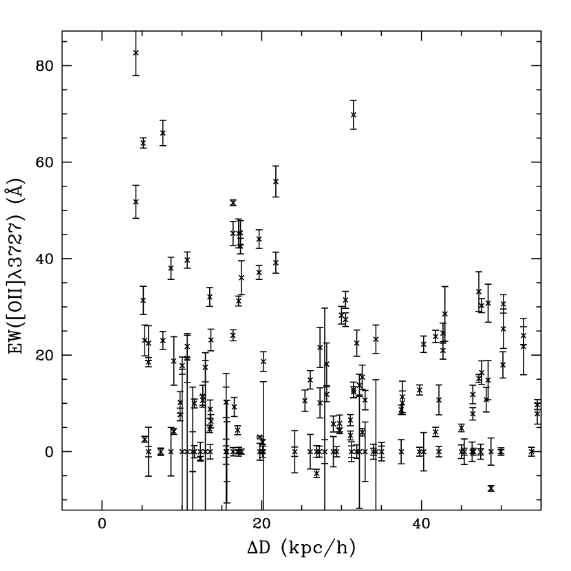
Figure 8: Same as Fig. 5, except that the ordinate is EW([OII]$\lambda 3727$).

Other emission lines are more accessible in high-$z$ systems. Figs. 7 – 9 show $\Delta D$ and $\Delta V$ vs equivalent widths for H$\beta$, [OII]($\lambda$3727) and [OIII]($\lambda$5007), including only galaxies in environments where $\rho_{2.5}\leq 2.2$. We omit one galaxy in Fig. 8 with no detection and huge error bars ($>50$ Å). The trends we observe in H$\alpha$ remain for each of these lines; Table 2 shows the Spearman rank probabilities of no trend for all of these lines and for H$\alpha$. The [OIII] correlation with $\Delta D$ is the strongest among the collisionally-excited lines.

As we note in Sec. 2, the CfA2North subsample is biased toward galaxies with emission lines, although the line-emitting fraction of the CfA2North subsample is unbiased with respect to the line-emitting fraction of the CfA2South subsample. The dearth of non-line-emitting galaxies is unlikely to affect the correlation, because these galaxies are distributed roughly evenly in $\Delta D$ in both the North and South. However, as a final check that the correlation we detect is real, we also restrict our test to the unbiased sample of galaxies with ${\rm EW}({\rm H}\alpha)>0$ and $\rho_{2.5}\leq 2.2$. This subsample includes only 106 galaxies, greatly reducing the ability of the Spearman rank test to detect the correlation. Nevertheless, P${}_{\rm SR}=7.0\times 10^{-2}$ and P${}_{\rm SR}=1.3\times 10^{-2}$ for $\Delta D$ – EW(H$\alpha$) and $\Delta D$ – EW(HeI) correlations, respectively. The stronger HeI correlation is consistent with the association between HeI and more recent star formation. The significance of the trends for other lines and for $\Delta V$ is greatly reduced. We record these statistics in Table 2.

Any complete sample of galaxies in pairs undoubtedly contains galaxies which do not show this starbursting effect because (1) they are interlopers, (2) they have not yet reached the stage at which the burst will begin, or (3) they are not gas-rich. Therefore, the correlations between emission line properties and orbit parameters in complete samples of optically-selected pairs may be weak. However, we conclude on the basis of rigorous tests that the emission line properties of galaxies in pairs correlate with $\Delta D$, independent of any sampling biases we detect. The correlations are not the result of large-scale environmental effects, such as gas stripping or the morphology-density relation. We conclude that these correlations arise from local, tidal interactions.

The correlations in our data are completely model-independent. However, recent simulations suggest a physical basis for them (Sec. 5). In the MH96 simulations, close orbital passes induce bursts of star formation in galaxies with shallow central potentials. These models essentially predict that emission-line properties of galaxies in pairs should depend on the local physics, including the parameters of the orbit. The correlations we find show that the local physics has a substantial affect on the emission properties of galaxies in pairs.

7 Starburst Models of Orbiting Galaxies

Here, we show that the correlation between $\Delta D$ and EW(H$\alpha$) can plausibly arise when a close pass between the galaxies triggers a burst of star formation which continues as the galaxies move apart. As the burst continues, EW(H$\alpha$) decreases as the new population raises the continuum around H$\alpha$. Roughly, $\Delta D$ increases and EW(H$\alpha$) decreases after the close pass, giving rise to the correlation.

We apply the starburst models of Leitherer et al. (1999; L99 hereafter; upgraded versions of the models in Leitherer & Heckman 1995). In Sec. 7, we use the L99 models and the EW(H$\alpha$) measurement in each galaxy to estimate the time since a recent starburst began, $t_{\rm burst}$. In Sec. 8, we discuss some consistency checks of the model, and in Sec. 9 we discuss sources of scatter and offsets in the transformation from an EW(H$\alpha$) to a $t_{\rm burst}$ or to a time since a close pass between the galaxies, $t_{\rm pass}$.

7.1 The Leitherer et al. Models

L99 model a starburst by “forming” stars according to an initial mass function (IMF) $\frac{\rm dN}{\rm dm}=C{\rm m}^{-\alpha}$, where m is the stellar mass, $\alpha$ is the slope of the IMF, and $C$ is a constant. They use models from the literature or construct their own models for stellar evolution, stellar atmospheres, and nebular emission. They compute spectral features, including EW(H$\alpha$), as a function of time for both the “instantaneous” starburst case, with a timescale $\tau\lesssim 10^{6}$ years, and the continuous case, with star formation over $10^{9}$ years.

The L99 models have a range of metallicity (0.05 Z_☉, 0.2 Z_☉, 0.4 Z_☉, Z_☉, 2Z_☉). The models also have a range of IMFs, including an approximate Salpeter (1955) IMF, with $\alpha=2.35$, from 1 M_☉ – 100 M_☉, a Salpeter IMF with a 30 M_☉ high-mass cutoff, and an approximate Miller-Scalo (1979) IMF with $\alpha=3.3$ from 1 M_☉ – 100 M_☉. Hereafter, we refer to these IMFs as Salpeter, cutoff Salpeter, and Miller-Scalo, respectively. In the continuous Miller-Scalo case, there are only very slight differences in EW(H$\alpha$) as a function of time between the Leitherer & Heckman (1995) model and the L99 model.

7.2 Measuring the Time Since the Burst Began With H$\alpha$

We use the model results from L99 to convert EW(H$\alpha$) for each galaxy in an environment with $\rho_{2.5}\leq 2.2$ to an estimated time since the burst began, $t_{\rm burst}$. Inclusion of the points with $\rho_{2.5}>2.2$ has no qualitative effects on the results. EW(H$\alpha$) decreases monotonically with time. Thus, the Spearman rank test significance of the $\Delta D$ – $t_{\rm burst}$ correlation under these assumptions should be the same as that of the $\Delta D$ – EW(H$\alpha$) correlation (Sec. 6). We begin applying the models assuming that the measured EW(H$\alpha$) depends on timescale according to the L99 models — that no significant older population contributes to the continuum around H$\alpha$. Because of possible contributions from old populations, EW(H$\alpha$) is a lower limit to the EW(H$\alpha$) due to the burst alone, and the $t_{\rm burst}$ we compute is an upper limit to the true time since the burst, in the context of the L99 models.

Barton et al. (1999b) use photometry of 190 galaxies in the spectroscopic sample and longslit spectra of 84 spirals and S0s to investigate the possible effects from an old stellar population. They apply the Leitherer et al. (1999) starburst models to measure s_R, the fractional $R$-band flux of the new burst, and $t_{\rm burst}$, the elapsed time since the burst began. With their assumptions about the color of the old stellar population and the reddening correction (based on the observed Balmer decrement), the Leitherer et al. (1999) Miller-Scalo IMF models imply large burst strengths ($0.2\lesssim{\rm s}_{\rm R}\lesssim 1$) in the centers of some of the galaxies. The burst strength, s_R, may depend on at least one internal parameter of the galaxies, the velocity width. The interaction-related parameters appear to determine $t_{\rm burst}$; the measured values of $t_{\rm burst}$ correlate significantly with $\Delta D$, the projected pair separation on the sky. Thus, although their conclusions are somewhat sensitive to assumptions about reddening, the IMF of the new burst, and the color of the old stellar population, Barton et al. (1999b) show that in many galaxies, the burst population may constitute a significant fraction of the $R$-band flux ($\gtrsim 20\%$, and up to $\sim$100%). For bursts of this strength, contributions from the old stellar population have only a small effect on the measured $t_{\rm burst}$. Thus the approach we take here of ignoring the old population should give a reasonoble indication of the relationship between $t_{\rm burst}$ and the kinematic parameters of the interaction.

We apply the two star formation models of L99: the instantaneous burst and the continuous burst. The star formation rate probably depends on the interaction strength and the galaxy potential (MH96); however, Leitherer & Heckman (1995) show that these two cases successfully bracket the properties of intermediate cases. Later, we apply consistency checks and discuss complications which affect the interpretation of the results.

Fig. 10 shows $t_{\rm burst}$ computed with a Miller-Scalo IMF with Z$=$Z_☉ and continuous star formation. Fig. 10a shows $\log({\rm EW}({\rm H}\alpha))$ as a function of $\Delta D$ for the line-emitting galaxies. We correct EW(H$\alpha$) for Balmer absorption because L99 do not account for it in their computation. Fig. 10b shows the log of the corresponding time in years since initiation of the burst; we convert each equivalent width to a $t_{\rm burst}$ using simple linear interpolation of the L99 points. In this and all similar plots, we exclude galaxies with $t_{\rm burst}>10^{9}$ years: the L99 models do not extend past 1 Gyr.

This correlation between $\Delta D$ and $t_{\rm burst}$ depends only on our assumptions about the behavior of the burst population and the contribution of other populations to the spectrum; it is independent of the predictions of the n-body models. However, if it does indicate that pairs with larger $\Delta D$ have older bursts, what were the (spatial) properties of the galaxies when the bursts were younger? Presumably, they were similar to the youngest bursts now: they had small pair separations ($\Delta D$). Thus, the interpretation based on the MH96 models follows naturally: bursts are initiated at small $\Delta D$ and age as the galaxies move apart.

If interaction between the two galaxies in each pair did give rise to a starburst which resulted in the observed EW(H$\alpha$), the current separation of the galaxies and the elapsed $t_{\rm burst}$ should provide information about the average velocity of the pair in the sky plane. Thus, in Fig. 10b we plot contours of “average velocity”, $\bar{v}_{\bot}$, in the plane of the sky, where $\bar{v}_{\bot}=\Delta D/$$t_{\rm burst}$. Although we cannot measure either component of this velocity for independent comparison, the size of our sample allows statistical estimation of the appropriate velocity range. The range is $\sim\sqrt{2}\times(50$ – $200$ km/s), assuming no preferred orientation of orbits, based on the distribution of the line-of-sight velocity separation for pairs with H$\alpha$ (Fig. 11). In the next section, we explore the expected distribution in detail.

If the starburst began at exactly the time of a very close pass, the time at which $\Delta D\approx 0$ for each pair, $\bar{v}_{\bot}$ is the average relative velocity of the pair in the plane of the sky since the close pass. For nonzero impact parameter ($\Delta D=b\neq 0$ at closest approach), the $\bar{v}_{\bot}$ contours should be shifted to the right by the value of $b$. The dotted contours are $\bar{v}_{\bot}$ shifted by $b=4{\rm\ h}^{-1}$ kpc, approximately the maximum 3-dimensional $b$, and hence the maximum 2-dimensional $b$, such that the 3-dimensional turnaround radius of the orbit is $\leq 50{\rm\ h}^{-1}$ kpc according to our rough orbit models (see Sec. 7.3). Thus, in the context of our orbit model, the range between the solid and dotted contours roughly represents the expected scatter due to nonzero $\Delta D$ at closest approach.

The essence of this analysis is the comparison of the starburst timescale with the dynamical timescale in these systems. This approach has been successful in the past, when applied to small numbers of mergers with burst ages estimated from the star cluster populations (Whitmore et al. 1997 and references therein). Fig. 10b shows that the scales match appropriately; the points with the largest EW(H$\alpha$) in Fig. 10b have relative velocities in the plane of the sky (corresponding to the contours) which fall very nearly in the proper range, $\lesssim 50$ km/s to $\sim 400$ km/s, roughly as expected from the independent line-of-sight relative velocities (Fig. 11). The plot shows one outlier, the starburst nucleus UGC 2103, at $\geq 800$ km/s. The shape of the lower edge of the locus of the points with large EW(H$\alpha$) is a good match to an approximately constant velocity of $\sim 400$ km/s. Next, we explore the expected distribution of points in this $\Delta D$-$t_{\rm burst}$ plane based on simple orbit models. In Sec. 7.4, we apply the other variants of the L99 models.

7.3 Comparing the Data to Orbit Models

The expected distribution of $\bar{v}_{\bot}$ for a sample of orbiting pairs depends on the population of the orbits and on the effects of dynamical friction (Turner 1976a; 1976b; Bartlett & Charlton 1995). Fig. 12 shows the distribution in the $\Delta D$ – $t_{\rm burst}$ plane for a population of galaxies just after the first pass for orbits with zero initial orbital energy and with the characteristics listed in the figure caption. In each figure, we include 19 orbits with a range of impact parameters at first pass, $b=2$ – 24 h^-1 kpc in increments of  1.3 h^-1 kpc (we assume H₀ = 65 km/s/Mpc to convert from kpc in the models to the units of observation, h^-1 kpc). We weight orbits by $b_{\rm Kep}$, the value of $b$ in the absence of dynamical friction, to account for the larger probability of a larger impact parameter. We compute the orbits using a rough implementation of the Chandrasekhar dynamical friction formula (Chandrasekhar 1943; Binney & Tremaine 1987) for isothermal spheres. We tune the calculation for a very rough match to orbits based on the self-consistent n-body models of Barton et al. (1999a).

Other orbit families with varied amounts of initial orbital energy and/or varied galaxy masses occupy loci on Fig. 12 with similar shapes, but the quantitative locations of the edges of the point distribution change substantially. Without a priori knowledge of galaxy masses and initial orbital energies, as well as detailed treatment of dynamical friction, we cannot construct an accurate set of orbit models to match to the data precisely. Qualitatively, however, the models show that a population of orbits fills in a region with a shape similar to the one occupied by the data in Fig. 10b.

7.4 Other L99 Models

Figs. 13 and 14 show $t_{\rm burst}$ estimates for the L99 models with Z=0.4 Z_☉, Z=Z_☉ and 2 Z_☉ in the continuous and instantaneous cases, respectively. The Miller-Scalo and cutoff Salpeter IMFs match better than the Salpeter IMF. The Salpeter IMF points mostly fall above the graph — the Salpeter IMF predicts values of EW(H$\alpha$) much larger than those in our sample, suggesting that massive stars are overabundant in the Salpeter IMF. For the instantaneous models, the required velocities in the sky plane are generally $>1000$ km/s, much too large.

However, direct comparison between Figs. 13 – 14 and Fig. 12 assumes that the starburst began exactly at the time of the close pass, or $t_{\rm burst}=t_{\rm pass}$. In the MH96 models, the burst is delayed until $\sim$100 Myr after the pass. Fig. 15 shows times computed with an instantaneous model ($\alpha=3.3$ IMF with Z$=$Z_☉), including delays in the starburst of $t_{\rm delay}=$ $t_{\rm pass}$ - $t_{\rm burst}=$ 0, 5 Myr, 40 Myr and 200 Myr. The y-axis in these plots is now the time since the close pass, $t_{\rm pass}$, not the time since the starburst; thus, the same $\bar{v}_{\bot}$ contours still apply. A delay in the burst can boost the points into the appropriate range of $\bar{v}_{\bot}$, but the model no longer explains the observed EW(H$\alpha$) distribution.

In the instantaneous models, a large range in EW(H$\alpha$) corresponds to only a small range of $t_{\rm burst}$. Thus, if these instantaneous models were correct, most of the observed equivalent widths would correspond to $t_{\rm burst}\approx 10^{7}$ years, and would represent only a brief snapshot in the interaction process. If the instantaneous models were correct, something entirely different would be responsible for the anti-correlation of $\Delta D$ and EW(H$\alpha$), such as an unlikely correlation between $t_{\rm delay}$ and $\Delta D$ that is fine-tuned to time differences of 10⁷ years. We conclude that, barring significant problems with the conversion from EW(H$\alpha$) to $t_{\rm burst}$, the instantaneous models are excluded by the data — starbursts due to interaction must be extended in time ($\tau\gg 10^{6}$ years and probably $\tau\gtrsim 10^{8}$ years).

Because delays between the close pass and the burst may be a generic feature of tidally-triggered starbursts, we explore delays in the continuous case as well. In Fig. 16 we plot $t_{\rm pass}$ for $t_{\rm delay}$ = 0, 5 Myr, 40 Myr, and 200 Myr in the continuous models. Large delays drastically change the locus of the points in the $\Delta D$ – $t_{\rm pass}$ plane derived from the models. The proper way to compare Fig. 16 to Fig. 12 is to ignore the points in Fig. 12 with $t_{\rm pass}<$$t_{\rm delay}$; these points correspond to pre-burst galaxies where the EW(H$\alpha$) does not yet reflect the close pass. In this picture, the observed distribution allows only a moderate delay. Similarly, the data do not rule out bursts initiated a very short time before closest approach.

The larger delays, with $t_{\rm delay}\gtrsim 50$ Myr, change the shape of the distribution until it no longer tracks the shape of the constant-velocity contours, and the model no longer explains the correlation between EW(H$\alpha$) and $\Delta D$. If our interpretation is correct, the data admit only the Miller-Scalo and cutoff Salpeter IMFs with continuous star formation.

8 Consistency Checks for the Model

Secs. 5 – 7 suggest a simple interpretation of our pair data that agrees with qualitative results from n-body/SPH simulations (MH96), starburst models (L99), and simple orbit models. In Sec. 7 we show that timescales based on the several L99 models match the dynamical timescales for a family of orbits, explaining the observed $\Delta D$ – EW(H$\alpha$) correlation. This picture has implications for other aspects of the data which we explore here, including the $\Delta V$ distribution as a function of $t_{\rm pass}$, the strength of Helium lines, and the presence of Balmer absorption.

8.1 Comparing to the $\Delta V$ Distribution

To this point, we have not used the measured velocity separation, $\Delta V$, in our models. In Fig. 17 we plot the expected $\Delta V$ vs. $t_{\rm pass}$ for the orbits of Fig. 12. At apogalacticon, the range of $\Delta V$ values is very tight around zero; before and after, the range is much broader. The apogalacticon time changes somewhat for different orbital energies or different galaxy masses.

We plot $\Delta V$ vs. $\log(t_{\rm pass})$ for the data in Fig. 18, using the L99 model of Fig. 10b, with $\alpha=3.3$, Z=Z_☉, continuous star formation, and no delay (Fig. 18a). Qualitatively, the distribution of the points is similar to the predicted distribution (Fig. 17): the velocity separations are spread out for small $t_{\rm burst}$, especially for the HeI-emitting galaxies. The velocity separations squeeze in at $\log(t_{\rm pass,apo})\sim 8.2$, and spread out again at later times. However, the exact value of $t_{\rm pass,apo}$ is not determined by our data: a delay, a different model, or any physical process that can change the mapping from EW(H$\alpha$) to $t_{\rm pass}$ can change the $t_{\rm burst,apo}$ derived from the data.

8.2 After the Starburst

If the galaxies with large H$\alpha$ equivalent width are starbursting galaxies observed just after a close pass, where are the post-starburst galaxies? Only one galaxy in our spectroscopic sample, NGC 7715, has a classical “E+A” spectrum, with a very blue continuum, no emission whatsoever, and huge EW(H$\delta$)$=-7.7$, but several galaxies show detectable H$\delta$ absorption, consistent with a fading, $\sim$$10^{9}$-year-old starburst, when the galaxies should be at or past apogalacticon. Thus, we might expect these post-burst candidates to have a range of $\Delta D$ values, determined largely by the range of apogalacticon distances populating the sample (see the range of $\Delta D$ for $t_{\rm pass}\approx 10^{9}$ in Fig. 12). However, if these galaxies are clumped near apogalacticon, their $\Delta V$ distribution would be narrower than for pairs at other stages (see the smaller range of $\Delta V$ for $t_{\rm pass}\approx 10^{9}$ in Fig. 17).

Fig. 19 shows normalized histograms of $\Delta D$ and $\Delta V$ for the 46 galaxies in our low-density ($\rho_{2.5}\leq 2.2$) sample with EW(H$\delta$) $<-2$ Å (solid line) and for the 85 galaxies in our low-density sample with EW(H$\delta$) $\geq 0$ (dotted line). K-S tests show that the $\Delta D$ distributions are the same at the 24% level. However, the $\Delta V$ distributions differ at the 11.7% level, and at the 3.7% level if restricted to $\rho_{2.5}\leq 2.0$. The distribution for the points with EW(H$\delta$)) $<-2$ Å is clearly shifted towards smaller $\Delta V$, consistent with a population of galaxies near apogalacticon.

NGC 7715, the true “E+A” galaxy, is paired with the Wolf-Rayet galaxy NGC 7714 ($\Delta V=49$ km/s). NGC 7714 shows a ring-like distortion likely associated with a very close pass, or even a penetrating encounter (see, e.g., Papaderos & Fricke 1998 for a detailed discussion).

8.3 Helium

HeI is a recombination line which provides further constraints on and consistency checks of the application of the L99 star-formation models. The relative strength of HeI can be estimated directly from the expected number of ionizing photons given in the L99 models. The relative strength of HeI provides a good consistency check — in some of the L99 models, the predicted ratio of HeI/H$\alpha$ matches the data well for the young starbursts.

Under the assumption that the nebulae surrounding the massive stars are optically thick to all photons in the Lyman and HeI continuum, and that radiative transfer effects are negligible, the ratio HeI/H$\alpha$ can be estimated from the relevant photon populations and recombination coefficients, assuming n${}_{\rm e}=10^{4}{\rm\ cm}^{-3}$ and T${}_{\rm e}=10^{4}$ K, where n_e and T_e are the electron density and temperature, respectively. The HeI($\lambda$5875)/H$\alpha$ ratio under these assumptions is 0.28 N(He⁰)/N(H⁰), where N(He⁰) and N(H⁰) are the number of photons capable of ionizing HeI and HI, respectively (Osterbrock 1989).

The L99 models predict both N(He⁰) and N(H⁰). Fig. 20 shows a grid of 0.28 N(He⁰)/N(H⁰), or the predicted HeI/H$\alpha$, as a function of time from L99. Each plot shows the continuous (solid line) and instantaneous (dotted line) bursts. The L99 models predict that HeI emission should disappear very rapidly after a burst, in $\lesssim 10^{7}$ years. In continuous star-forming mode, HeI/H$\alpha$ stays roughly constant; the ratio deviates from its continuous mode only when the star formation begins or ceases.

Fig. 21a shows HeI/H$\alpha$ vs. EW(H$\alpha$) for pair galaxies in low-density environments ($\rho_{2.5}\leq 2.2$) in our sample with EW(H$\alpha$)$>10$Å. We correct HeI/H$\alpha$ for 0.5 Å of stellar absorption in Fig. 21a (T. Heckman, private communication), although we neglect the effects of this small correction in Fig. 21b (and in Sec. 6). The x axis is inverted; younger starbursts are to the left. The galaxies with the largest EW(H$\alpha$) cluster around HeI/H$\alpha$ = 0.04 – 0.05, as predicted by several of the models in Fig. 20. Most notably, the best matches are for the 2 Z_☉ Salpeter model, and the Miller-Scalo model with Z = 1 – 2 Z_☉. The cutoff Salpeter model predicts HeI/H$\alpha$ $\leq 0.02$ for these metallicities, which is below the measured values. However, these results should be interpreted with caution. L99 and Leitherer & Heckman (1995) note that N(He⁰) is very sensitive to metallicity variations. Their models are not chemically self-consistent — the stellar populations maintain the same metallicity throughout the calculation.

The scatter in HeI/H$\alpha$ increases for the older starbursts. This increase could have many causes, including variations in metallicity, increased dust, or the inadequacy of the assumptions relating HeI/H$\alpha$ to N(He⁰)/N(H⁰). Additionally, for small EW(H$\alpha$), non-Gaussian errors could contribute more significantly (e.g. problems with the correction for Balmer absorption which are not reflected in the error bars). However, if these possibilities could be eliminated, the HeI/H$\alpha$ ratio could serve as an indicator of an abrupt change in the star formation rate.

In Fig. 21b we show upper limits to HeI/H$\alpha$ for several galaxies with H$\alpha$ emission but no detected HeI. In most cases, the limits are consistent with the values in Fig. 21a. However, a few upper limits, as well as a few HeI/H$\alpha$ ratios in Fig. 21a, are quite small and should be investigated as systems where star formation may have ceased within the last $\sim$10⁷ years.

In summary, the behavior of HeI generally agrees with the predictions of the L99 models, especially some of the Miller-Scalo and Salpeter IMF models. If the models predict the correct HeI/H$\alpha$, which depends on the detailed treatment of the most massive stars and is therefore currently uncertain, the measured HeI/H$\alpha$ distribution can distinguish between the cutoff Salpeter and Miller-Scalo IMFs, which both roughly match the $\Delta D$-$t_{\rm burst}$ distribution (see Sec. 7); the (uncertain) predictions of L99 favor the Miller-Scalo IMF. Additionally, outliers in the HeI/H$\alpha$ distribution may be galaxies which have undergone a recent, abrupt change in the star formation rate.

9 Discussion

A large number of effects, in addition to model inaccuracy, can lead to scatter in the transformation from an H$\alpha$ equivalent width to a $t_{\rm burst}$, as well as to a $t_{\rm pass}$. Here, we estimate the scatter in the transformation and mention the effects of old stellar populations and different galaxy potentials.

Paired galaxies, if they are truly interacting, have identical values of the time since a close pass, $t_{\rm pass}$. If the delay between the pass and the induced starburst is the same for the two galaxies, if neither have significant contamination at H$\alpha$ from an old stellar population, and if both have available gas, the galaxies in the pair should have identical EW(H$\alpha$). Kennicutt et al. (1987) report a correlation of EW(H$\alpha$) in galaxies in the same pair, which they note is similar to the “Holmberg effect” for concordance in galaxy colors (Holmberg 1958; Madore 1986).

Some pairs in our sample have very similar EW(H$\alpha$); others have widely discrepant values. Fig. 22a shows EW(H$\alpha$) as a function of $\Delta D$ with points in the same pair connected; we restrict the sample to galaxies in environments with $\rho_{2.5}\leq 2.2$ and include only pairs (no n-tuples) for simplicity. The median scatter in EW(H$\alpha$) for these 66 pairs is 8.7 Å.

We test the significance of similarity in EW(H$\alpha$) using a Monte Carlo simulation in which we scramble the EW(H$\alpha$) values among the relevant pairs. We compare the true distribution of scatter in EW(H$\alpha$) to the Monte Carlo version (from 500 scramblings) in Fig. 22b. The true distribution includes a clear excess near zero; a K-S test indicates that the distributions differ significantly, at the 0.05% level.

We roughly test the possibility that the apparent concordance may arise from the $\Delta D$ – EW(H$\alpha$) correlation alone, since galaxies in pairs always have the same $\Delta D$. We apply the test to just the 27 pairs with $\Delta D<20{\rm\ h}^{-1}$ kpc and the 28 pairs $\Delta D>30{\rm\ h}^{-1}$ kpc; the observed distributions differ from the scrambled Monte Carlo distributions at the 1.5% and 2.5% levels, respectively. We conclude, in agreement with Kennicutt et al. (1987), that EW(H$\alpha$) is correlated for galaxies in the same pairs; this concordance is probably not just an artifact of the $\Delta D$ – EW(H$\alpha$) correlation.

When comparing the points to the models in Sec. 7, the appropriate quantity to consider for each pair is the largest EW(H$\alpha$) in the pair. Most factors serve only to reduce EW(H$\alpha$) “artificially”. One exception is the star formation normally associated with spiral galaxies, which will increase EW(H$\alpha$). In our sample, some of these factors can be explored directly, by comparing galaxies with their companions.

The most important factor affecting $t_{\rm burst}$ may be the presence of an old stellar population contributing to the continuum near H$\alpha$. If it does, EW(H$\alpha$) depends somewhat on the burst strength; a correlation could then arise between EW(H$\alpha$) and $\Delta D$ if pairs on small orbits have the strongest starbursts. However, Barton et al. (1999b) combine photometry with these spectra and use a two-population model for the stellar content of the galaxies to show that the $\Delta D$ – EW(H$\alpha$) correlation is at least partly a result of the presence of older bursts at larger $\Delta D$. This conclusion is relatively robust with respect to assumptions about reddening, the old stellar population, and the IMF. Using the L99 continuous Miller-Scalo model with Z=Z_☉, and some assumptions about the reddening and old stellar population, they also show that the strengths of many of the bursts are probably large. This analysis indicates that the old stellar population would move the locus of the points in Fig. 10b by only a few tenths of a unit along the y axis.

Photometry and rotation curves of the starbursting galaxies in our sample will provide a further check of the MH96 models (Barton et al. 1999c). The MH96 models show that the response of the gas to a close pass depends dramatically on the mass distribution of a galaxy. Observations that extend beyond the nuclear region (e.g. Kennicut et al. 1987) indicate that interactions can enhance the star formation in the disk, as well as the nucleus. Mihos (1997) models gas-rich, low surface brightness galaxies and shows that the tidally-triggered star formation is spatially extended. In the MH96 simulations of galaxies with steeper potentials, the galaxies with deep central potentials and bulges respond only minimally to a close pass, while close passes trigger starbursts in galaxies with shallow central potentials (on prograde orbits). Thus, if the picture from the simulations is correct, we expect the galaxies in our sample with nuclear bursts of star formation to have no bulges and shallow inner rotation curves; galaxies with extended star formation should have even shallower rotation curves. Longslit, major axis rotation curves taken at the MMT (Barton et al. 1999c) of some of the emission-line galaxies in our sample show qualitatively that the brightest few starbursts have shallow rotation curves, with small velocity widths, suggesting that their central potentials are shallow and their total masses are small.

Orbital inclination also affects the response of galaxies to tidal interaction. Toomre & Toomre (1972) initially realized that in galaxy collisions, distortion is induced by resonant interactions. Thus, the differences in response between prograde and retrograde galaxies are dramatic — retrograde galaxies show almost no tidal or kinematic distortions. However, Keel (1993) reports no detectable differences in EW(H$\alpha$) between statistical samples of 27 mostly prograde and 21 mostly retrograde galaxies in pairs. MH96 report that retrograde encounters can trigger star formation in simulations, although they do not produce dramatic tidal tails. Preliminary results from our sample indicate that prograde and retrograde encounters have similar emission-line characteristics, although the prograde encounters appear to produce different tidal features.

We plan to discuss these issues in more detail by incorporating B and R images and rotation curves into the analysis (Barton et al. 1999c). We will include a detailed analysis of the surface brightness profiles and colors of the galaxies, a measure of the steepness of the rotation curves, and a comparison of the prograde and retrograde encounters in our sample.

10 Conclusion

We analyze 502 new optical spectra of galaxies in pairs and n-tuples in the original CfA2 redshift catalog, selected to have projected separations $\Delta D\leq 50$h^-1 kpc, velocity separations $\Delta V\leq 1000$ km/s, no isolation criteria, and redshifts $cz\geq 2300$ km/s. The sample includes the complete set of pairs in the original CfA2South survey and 45% of all of the 1115 known galaxies in pairs and n-tuples in the region with m${}_{\rm Zw}\leq 15.5$, included in the refined version of the CfA2 survey (Falco et al. 1999).

150 galaxies have significant emission in the four main diagnostic lines: H$\alpha$, H$\beta$, [OIII]($\lambda 5007$) and [NII]($\lambda 6584$). Starbursts and HII-region galaxies are common among these galaxies, but there is no evidence for the excess of AGNs observed among luminous infrared galaxies. Only 13% of the emitting galaxies in our sample have emission-line ratios consistent with Seyferts or LINERS, compared with 41% of the LIG sample of Veilleux et al. (1995). Conversely, the pair sample contains a population of “extreme starbursting galaxies” absent from the LIGs of Veilleux et al. (1995).

The equivalent widths of H$\alpha$ and other emission lines depend strongly on pair $\Delta D$ and $\Delta V$ (e.g., Kennicutt et al. 1987). These (anti-)correlations are not merely a result of large-scale environmental effects that we detect; nor does the correlation result from other sample biases. If we assume EW(H$\alpha$) for an isolated burst of star formation decreases monotonically with time, as starburst models like L99 suggest, and that this change in age dominates the $\Delta D$ – EW(H$\alpha$) correlation (Barton et al. 1999b), then the correlation shows that galaxies in pairs with larger separations tend to have older starbursts.

By matching the dynamical timescale to the burst timescale (L99), we show that the anti-correlation between $\Delta D$ and EW(H$\alpha$) can arise from bursts of star formation initiated just after perigalacticon, because EW(H$\alpha$) decreases with time as the pair separation increases. Our data show remarkable consistency with this picture:

1. EW(H$\alpha$) is highly correlated for galaxies in the same pair, consistent with the fact that local interactions determine the star-forming properties of galaxies in our sample (Kennicutt et al. 1987; for colors, see Holmberg 1958; Madore 1986).

2. The data agree with the expected distribution of a population of orbiting galaxies in the $\Delta D$ – $t_{\rm burst}$ plane for a Miller-Scalo or a cutoff (M$\leq 30\$M_☉) Salpeter initial mass function, assuming that the contribution to the continuum at H$\alpha$ from a very old stellar population is minimal compared to the contribution from the most recent burst. The L99 Miller-Scalo model also predicts the HeI-to-H$\alpha$ ratios observed in our sample.

3. The data agree qualitatively with the expected distribution of galaxies in the $\Delta V$ – $t_{\rm burst}$ plane.

4. We record a population of galaxies with Balmer absorption that are candidate post-burst systems; their $\Delta V$ distribution is narrower than the $\Delta V$ distribution of the other pairs, consistent with a population of galaxies at apogalacticon, $\sim$$5\times 10^{8}$ – $10^{9}$ years after a close pass.

The remarkable agreement between the data and many aspects of the model shows that the dynamical timescales of the pairs match the burst timescales inferred from EW(H$\alpha$). The model is compatible with bursts of star formation induced by close passes as long as the bursts last longer than $\sim$10⁸ years and the delays between the close passes and the initiations of the bursts are less than a few$\times 10^{7}$ years. N-body/SPH simulations (MH96) provide a physical basis for this picture, predicting some starbursting galaxies in pairs; the simulations show that close interactions between galaxies can initiate bursts of star formation before the final merger if the galaxies have shallow central potentials. These starbursts should be visible while the galaxies are a resolvable pair.

The picture we develop here, in conjunction with a large sample of spectroscopic and photometric data, along with rotation curves, has great potential for constraining the IMF and the duration of tidally-triggered starbursts, the true fraction of interacting galaxies in pairs, the orbits, and the dynamical timescales of the interactions.

Table 1: K-S Tests of North/South Sample Differences

Distribution	Ngal North	Ngal South	K-S Probability
EW(H$\alpha$), all galaxies	192	310	$1.3\times 10^{-2}$
EW(H$\alpha$), H$\alpha$-emitting galaxies	103	128	$3.8\times 10^{-1}$
$\Delta D$, all galaxies	192	310	$1.2\times 10^{-2}$
$\Delta D$, H$\alpha$-emitting galaxies	103	128	$2.0\times 10^{-1}$
$\Delta D$, non-H$\alpha$-emitting galaxies	89	182	$1.5\times 10^{-1}$
$\Delta V$, all galaxies	192	310	$3.1\times 10^{-2}$
$\Delta V$, H$\alpha$-emitting galaxies	103	128	$2.4\times 10^{-2}$
$\Delta V$, H$\alpha$-emitting galaxies, low density	56	50	$5.2\times 10^{-3}$

Note. — K-S tests of the differences between the North and South distributions of EW(H$\alpha$), $\Delta D$, and $\Delta V$ for the full sample and for various subsamples.

Table 2: Spearman Rank Probabilities of No Correlation

	All Densities		$\rho_{2.5}\leq 2.2$		$\rho_{2.5}\leq 2.2$, With H$\alpha$
	(502 galaxies)		(162 galaxies)		(106 galaxies)
Line	$\Delta D$ – EW	$\Delta V$ – EW	$\Delta D$ – EW	$\Delta V$ – EW	$\Delta D$ – EW	$\Delta V$ – EW
H$\alpha$	$5.2\times 10^{-3}$	$6.3\times 10^{-5}$	$1.7\times 10^{-2}$	$1.9\times 10^{-3}$	$7.0\times 10^{-2}$	$2.8\times 10^{-1}$
H$\beta$	$1.4\times 10^{-2}$	$4.2\times 10^{-4}$	$4.6\times 10^{-2}$	$5.4\times 10^{-3}$	$1.1\times 10^{-1}$	$1.5\times 10^{-1}$
HeI($\lambda 5876$)	$3.1\times 10^{-2}$	$9.7\times 10^{-3}$	$1.5\times 10^{-2}$	$1.4\times 10^{-2}$	$1.3\times 10^{-2}$	$1.6\times 10^{-1}$
OII ($\lambda 3727$)	$6.7\times 10^{-3}$	$5.8\times 10^{-5}$	$1.5\times 10^{-1}$	$4.1\times 10^{-3}$	$3.7\times 10^{-1}$	$9.1\times 10^{-2}$
OIII ($\lambda 5007$)	$1.6\times 10^{-3}$	$5.7\times 10^{-6}$	$3.6\times 10^{-2}$	$1.9\times 10^{-3}$	$9.4\times 10^{-2}$	$8.5\times 10^{-2}$

Note. — P_SR for possible correlations between orbit parameters ($\Delta D$,$\Delta V$) and equivalent widths (EWs) for various lines, including all the galaxies, all the galaxies in environments with $\rho_{2.5}\leq 2.2$, or only the galaxies with significant H$\alpha$ emission in environments with $\rho_{2.5}\leq 2.2$.

Figure 1: log([NII]$\lambda 6584$/H$\alpha$) vs. [OIII]$\lambda 5007$/H$\beta$ for emitting galaxies in our sample. Solid lines divide the sample into different types based on the empirical results of Veilleux & Osterbrock (1987). Circled points are galaxies with broad emission lines typical of Seyferts; their ratios are uncertain due to deblending problems. We label the population of $\sim$8 extreme starburst galaxies as ESBs.

Figure 2: EW(H$\alpha$) as a function of (a) $\Delta D$ (excluding points with $\Delta D>55$h^-1 kpc), and (b) $\Delta V$ (excluding points with $\Delta V>1000$ km/s).

Figure 3: EW(H$\alpha$) as a function of (a) systemic recession velocity, and (b) density of the surrounding environment, smoothed to 2.5h^-1 kpc and normalized to the survey mean.

Figure 4: Spearman rank probability of no correlation for galaxies in environments with $\rho_{2.5}<\rho_{\rm cut}$ as a function of $\rho_{\rm cut}$ for $\Delta D$ vs. EW(H$\alpha$) (solid line), $\Delta V$ vs. EW(H$\alpha$) (dashed line) and $\rho_{2.5}$ vs. EW(H$\alpha$) (dot-dashed line). The bottom panel shows the number of galaxies (with $\rho_{2.5}<\rho_{\rm cut}$) that contribute to each point.

Figure 5: Same as Fig. 2, restricted to galaxies in environments with $\rho_{2.5}\leq 2.2$.

Figure 6: Same as Fig. 5, except that the ordinate is EW(HeI$\lambda 5876$).

Figure 7: Same as Fig. 5, except that the ordinate is EW(H$\beta$).

Figure 9: Same as Fig. 5, except that the ordinate is EW([OIII]$\lambda 5007$).

Figure 10: (a) $\Delta D$ vs. log(EW(H$\alpha$)) for galaxies with EW(H$\alpha$)$\gtrsim 10$Å, and (b) the corresponding log($t_{\rm burst}$) from the L99 model with continuous star formation, Z=Z_☉ and a Miller-Scalo IMF. The solid contours are lines of constant average velocity in the plane of the sky; the dotted contours are offset by 4 h^-1  kpc. Only points with $t_{\rm burst}<10^{9}$ years appear in (b).

Figure 11: Line-of-sight velocity differences for galaxies in the sample with significant H$\alpha$ emission.

Figure 12: Orbit Models: $\Delta D$ vs. the log of the time since the most recent pass in years, log($t_{\rm pass}$), for a set of orbits with zero initial orbital energy, E${}_{0}=0$. The impact parameters are spaced uniformly from 2 – 24 h^-1 kpc, assuming H${}_{0}=65$ km/s/Mpc, and orbits are weighted by $b$ to account for the higher probability of a larger impact parameter. Points are at random times, viewed from random angles. The galaxy masses are M${}_{\rm gal}=5.8\times 10^{11}$ M_☉. The solid contours are lines of constant average velocity in the plane of the sky, for 50, 100, 200, 400 and 800 h^-1 km/s.

Figure 13: Same as Fig. 10b for a variety of L99 IMFs and metallicities, in the continuous star formation case. The solid contours are lines of constant average velocity in the plane of the sky,in units of h^-1 km/s; we omit the dashed lines of Fig. 10b for simplicity. S, CS, and M-S refer to the Salpeter, Cutoff Salpeter, and Miller-Scalo IMFs, respectively.

Figure 14: Same as Fig. 10b for a variety of L99 IMFs and solar metallicity, in the instantaneous star formation case. The solid contours are lines of constant average velocity in the plane of the sky,in units of h^-1 km/s. The plots appear very similar for $Z=0.4Z_{\sun}$ and $Z=2Z_{\sun}$. S, CS, and M-S refer to the Salpeter, Cutoff Salpeter, and Miller-Scalo IMFs, respectively.

Figure 15: $\Delta D$ vs. log($t_{\rm pass}$ ) from the L99 model with instantaneous star formation, Z=Z_☉ and a Miller-Scalo IMF, for different values of ${\rm t}_{\rm delay}={\rm t}_{\rm pass}-{\rm t}_{\rm burst}$. Only points with $t_{\rm pass}<10^{9}$ years appear. The solid contours are lines of constant average velocity in the plane of the sky,in units of h^-1 km/s.

Figure 16: Same as Fig. 15 for continuous star formation.

Figure 17: Orbit Models: $\Delta V$ vs. the log of the time since the closest pass in years, log($t_{\rm pass}$). The impact parameters are spaced uniformly from 2 – 24 h^-1 kpc, assuming H${}_{0}=65$ km/s/Mpc. Orbit sampling frequencies are weighted by $b_{\rm Kep}$ to account for the higher probability of orbits with larger impact parameters. Points are at random times, viewed from random angles. The open circles represent points just after the first close pass; the filled circles are just after the second close pass. The galaxy masses are M${}_{\rm gal}=5.8\times 10^{11}$ M_☉. The orbits have zero initial orbital energy.

Figure 18: $\Delta V$ vs. log($t_{\rm pass}$) from the L99 model with instantaneous star formation, Z=Z_☉ and a Miller-Scalo IMF, for ${\rm t}_{\rm delay}=0$. Only points with $t_{\rm pass}<10^{9}$ years and $\Delta V<550$ km/s appear.

Figure 19: Balmer absorption: (a) $\Delta D$ distributions of galaxies in low-density ($\rho_{2.5}\leq 2.2$) environments with EW(H$\delta)<-2$ Å (solid line) and EW(H$\delta)\geq 0$ (dotted line), and (b) $\Delta V$ distributions of the same subsamples. Note that the sample with EW(H$\delta)\geq 0$ includes both emission-line galaxies and absorption galaxies.

Figure 20: Predicted HeI$\lambda 5876$/H$\alpha$ as a function of time for the continuous (solid line) and instantaneous (dotted line) star formation models of L99. S, CS, and M-S refer to the Salpeter, Cutoff Salpeter, and Miller-Scalo IMFs, respectively.

Figure 21: Observed HeI/H$\alpha$ as a function of log(EW(H$\alpha$)) for EW(H$\alpha$)$>10$ Å: (a) measured ratios, and (b) upper limits for the remaining galaxies.

Figure 22: Pairs in environments with $\rho_{2.5}\leq 2.2$: (a) $\Delta D$ vs. EW(H$\alpha$ with galaxies in the same pair connected and (b) distribution of the EW(H$\alpha$) scatter for the 66 pairs (solid line) and a “random” Monte Carlo scatter (dotted line), computed by sampling from the same EW(H$\alpha$) distribution.

References

- (1)
- (2) Allen, D. A., Norris, R. P., Meadows, V. S., & Roche, P. F. 1991, MNRAS, 248, 528
- (3) Armus, L., Heckman, T. M., & Miley, G. K. 1989, ApJ, 347, 727
- (4) Ashby, M., Houck, J. R., & Hacking, P. B. 1992, AJ, 104, 980
- (5) Baldwin, J. A., Phillips, M. M., & Terlevich, R. 1981, PASP, 93, 5
- (6) Bartlett, R. E., & Charlton, J. C. 1995, ApJ, 449, 497
- (7) Barton, E. J., Bromley, B. C., & Geller, M. J. 1999a, ApJ, 511, L25
- (8) Barton, E. J., & Geller, M. J. 1999b, in preparation
- (9) Barton, E. J., et al. 1999c, in preparation
- (10) Binney, J., & Tremaine, S. 1987, Galactic Dynamics (Princeton: Princeton Univ. Press)
- (11) Borne, K. D., et al. 1999, preprint, astro-ph/9902293
- (12) Bushouse, H. A. 1986, AJ, 91, 255
- (13) Chandrasekhar, S. 1943, ApJ, 97, 255
- (14) Condon, J. J., Condon, M. A., Gisler, G., & Puschell, J. J. 1982, ApJ, 252, 102
- (15) Delgado, R. M. G., & Heckman, T. 1999, preprint, astro-ph/9903192
- (16) Dressler, A. 1980, ApJ, 236, 351
- (17) Donzelli, C. J., & Pastoriza, M. G. 1997, ApJS, 111,181
- (18) Dubinski, J., Mihos, J. C., & Hernquist, L. 1996, ApJ, 462, 576
- (19) Falco, E. E., Kurtz, M. J., Geller, M. J., Huchra, J. P., Peters, J., Berlind, P., Tokarz, S., & Elwell, B. 1999, PASP, 111, 438
- (20) Gao, Y., & Solomon, P. M. 1999, ApJ, 512, 99
- (21) Geller, M. J. & Huchra, J. P. 1989, Science, 246, 897
- (22) Giovanelli, R. & Haynes, M. P. 1985, AJ, 90, 2445
- (23) Giovanelli, R., Meyers, S. T., Roth, J., & Haynes, M. P. 1986, AJ, 92, 250
- (24) Giovanelli, R. & Haynes, M. P. 1989, AJ, 97, 633
- (25) Giovanelli, R. & Haynes, M. P. 1993, AJ, 105, 1271
- (26) Grogin, N. A., & Geller, M. J. 1998, ApJ, 505, 506
- (27) Hashimoto, Y., Oemler, A., Jr., Lin, H., & Tucker, D. L. 1998, ApJ, 499, 589
- (28) Haynes, M. P., Magri, C., Giovanelli, R. & Starosta, B. M. 1988, AJ, 95, 607
- (29) Hernquist, L., & Mihos, J. C. 1995, ApJ, 448, 41
- (30) Ho, L., Filippenko, A. V., & Sargent, W. L. 1997, ApJS, 112,315
- (31) Holmberg, E. 1958, Medd. Lund. Astron. Obs. Ser. 2, No. 136
- (32) Huchra, J. P., Geller, M. J., de Lapparent, V. & Corwin, H. G., Jr. 1990, ApJS, 72, 433
- (33) Huchra, J., & Burg, R. 1992, ApJ, 393, 90
- (34) Huchra, J. P., Geller, M. J. & Corwin, H. G., Jr. 1995, ApJS, 99, 391
- (35) Hughes, D. H., et al. 1998, Nature, 394, 241
- (36) Hummel, E. 1981, A&A, 89, L1
- (37) Jones, B., & Stein, W. A. 1989, AJ, 98. 1557
- (38) Joseph, R. D., Meikle, W. P. S., Robertson, N. A., & Wright, G. S. 1984, MNRAS, 209, 111
- (39) Kauffmann, G., Colberg, J. M., Diaferio, A., & White, S. D. M. 1999, MNRAS, 303, 188
- (40) Keel, W. C., Kennicutt, R. C., Hummel, E., & van der Hulst, J. M. 1985, AJ, 90, 708
- (41) Keel, W. C. 1993, AJ, 106, 1771
- (42) Keel, W. C. 1996, ApJS, 106, 27
- (43) Kennicutt, R. C., & Keel, W. C. 1984, ApJ, 279, L5
- (44) Kennicutt, R. C., Jr., Keel, W. C., van der Hulst, J. M., Hummel, E., & Roettiger, K. A. 1987, AJ, 95, 5
- (45) Kurtz, M. J., & Mink, D. J. 1998, PASP, 110, 934
- (46) Larson, R. B., & Tinsley, B. M. 1978, ApJ, 219, 46
- (47) Leech, K. J., et al. 1989, MNRAS, 240, 349
- (48) Leitherer, C., & Heckman, T. M. 1995, ApJS, 96, 9
- (49) Leitherer, C., et al. 1999, ApJS, in press (L99)
- (50) Liu, C. T., & Kennicutt, R. C., Jr. 1995a, ApJ, 450, 547
- (51) Liu, C. T., & Kennicutt, R. C., Jr. 1995b, ApJS, 100, 325
- (52) Lonsdale, C. J, Persson, S. E., & Matthews, K. 1984, ApJ, 287, 95
- (53) Madore, B. F. 1986, in Spectral Evolution of Galaxies, eds. C. Chiosi & A. Renzini (Reidel, Dordrecht), p. 97
- (54) Marzke, R. O., Huchra, J. P., & Geller, M. J. 1994, ApJ, 428, 43
- (55) Massey, P., Strobel, K., Barnes, J. V., & Anderson, E. 1988, ApJ, 328, 315
- (56) Massey, P., & Gronwall, C. 1990, ApJ, 358, 344
- (57) Mihos, J. C., & Hernquist, L. 1996, ApJ, 464, 641 (MH96)
- (58) Miller, G. E., & Scalo, J. M. 1979, ApJS, 41, 513
- (59) Osterbrock, D. E. 1989, Astrophysics of Gaseous Nebulae and Active Galactic Nuclei (Mill Valley: University Science Books)
- (60) Papaderos, P., & Fricke, K. J. 1998, A&A, 338, 31
- (61) Postman, M., & Geller, M. J. 1984, ApJ, 281, 95
- (62) Salpeter, E. E. 1955, ApJ, 121, 161
- (63) Sanders, D. B., & Mirabel, I. F. 1996, ARA&A, 34, 749
- (64) Sanders, D. B., Soifer, B. T., Elias, J. H., Madore, B. F.,Matthews, K., Neugebauer, G., & Scoville, N. Z. 1988, ApJ, 325, 74
- (65) Schmidt, M. 1959, ApJ, 129, 243
- (66) Sekiguchi, K., & Wolstencroft, R. D. 1992, 255, 581
- (67) Somerville, R. S., & Primack, J. R., & Faber, S. M. 1998a, preprint, astro-ph/9806228
- (68) Somerville, R. S., & Primack, J. R., 1998b, preprint, astro-ph/9811001
- (69) Steidel, C. C., Giavalisco, M., Pettini, M., Dickinson, M., & Adelberger, K. L. 1996, ApJ, 462, L17
- (70) Tonry, J. L., & Davis, M. 1979, AJ, 43, 393
- (71) Toomre, A., & Toomre, J. 1972, ApJ, 178, 623
- (72) Turner, E. L. 1976a, ApJ, 208, 20
- (73) Turner, E. L. 1976b, ApJ, 208, 304
- (74) Veilleux, S., & Osterbrock, D. E. 1987, ApJS, 63, 295
- (75) Veilleux, S., Kim, D.-C., Sanders, D. B., Mazzarella, J. M., & Soifer, B. T. 1995, ApJS, 98, 171
- (76) Vogeley, M. S. 1993, Ph.D. Thesis, Harvard University
- (77) Wegner, G., Haynes, M. P., & Giovanelli, R. 1993, AJ, 105, 1251
- (78) Whitmore, B. C., Miller, B. W., Schweizer, F., & Fall, S. M. 1997, AJ, 114, 1797
- (79)