What heats the bright H ii regions in I Zw 18?

Abstract

We have used the radiation field from a starburst population synthesis model appropriate for the brightest H ii region of I Zw 18 to perform a photoionization model analysis of this object. We have investigated whether, with the observed nebular density distribution as revealed by the HST images and a total stellar radiation compatible with the observed UV flux, one could reproduce the constraints represented by the observed ionization structure, the He ii $\lambda$4686/H$\beta$ ratio, the H$\alpha$ flux and the electron temperature indicated by the [O iii] $\lambda$4363/5007 ratio.

We have found that, even taking into account strong deviations from the adopted spectral energy distribution of the ionizing radiation and the effect of additional X-rays, the photoionization models yield too low a [O iii] $\lambda$4363/5007 ratio by about 30%. This discrepancy is significant and poses an interesting problem, which cannot be solved by expected inaccuracies in the atomic data. The missing energy may be of the same order of magnitude as the one provided by the stellar photons or lower, depending on the way it acts on the [O iii] $\lambda$4363 line.

Elemental abundance determinations in I Zw 18 are affected by this problem. Before the nature of the missing heating source and its interactions with the nebular gas are better understood it is, however, not possible to estimate the typical uncertainties by which standard empirical methods are affected.

Several side-products of our photoionization analysis of I Zw 18 are the following:

• We have been able to reproduce the intensity of the nebular He ii $\lambda$4686 using a stellar radiation field consistent with the observed Wolf-Rayet features in I Zw 18.

• We have shown that the bright NW H ii region in I Zw 18 does not absorb all the ionizing photons from the central star cluster, and that about half of them are available to ionize an extended diffuse envelope.

• The [O i] emission can easily be accounted for by condensations or intervening filaments on the line of sight.

• The intrinsic H$\alpha$/H$\beta$ ratio is enhanced by collisional excitation to a value of 3. Previous estimates of the reddening of I Zw 18 are therefore slightly overestimated.

• We give ionization correction factors appropriate for I Zw 18 that can be used for more accurate abundance determinations in this object once the electron temperature problem is better understood.

.

1 Introduction

The blue compact dwarf emission-line galaxy I Zw 18 is famous for being the most metal poor galaxy known so far. Its oxygen abundance is about 2% the solar value, as first shown by Searle and Sargent (1972), and then confirmed by many studies (e.g. Lequeux et al. 1979, French 1980, Kinman & Davidson 1981, Pagel et al. 1992, Legrand et al. 1997, Izotov et al. 1997b, Vílchez & Iglesias-Páramo 1998). Because of this, I Zw 18 has played an essential role in the determination of the primordial helium mass fraction. Also, due to its extreme properties, I Zw 18 has been a choice target for studies of star formation history in blue compact galaxies (Dufour & Hester 1990, Hunter & Thronson 1995, Dufour et al. 1996, De Mello et al. 1998, Aloisi et al. 1999), of the elemental enrichment in dwarf galaxies (Kunth & Sargent 1986, Kunth et al. 1995) and of the interplay between star formation and the interstellar medium (Martin 1996, van Zee et al. 1998). An important clue is the distribution of the oxygen abundance inside the H ii regions (Skillman & Kennicutt 1993, Vílchez & Iglesias-Páramo 1998) and in the neutral gas (Kunth et al. 1994, Pettini & Lipman 1995, van Zee et al. 1998). Another clue is the carbon and nitrogen abundance (Garnett et al. 1997, Vílchez & Iglesias-Páramo 1998, Izotov & Thuan 1999). On the whole, there is a general consent about an intense and recent burst of star formation in I Zw 18 - which provides the ionizing photons - following previous star formation episodes. How exactly has the gas been enriched with metals during the course of the evolution of I Zw 18 remains to be better understood.

Much of our understanding (or speculations) on the chemical evolution of I Zw 18 (and other galaxies in general) relies on the confidence placed in the chemical abundances derived from the lines emitted in the H ii regions. These are generally obtained using standard, empirical, methods which have been worked out years ago, and rely on the theory of line emission in photoionized gases. Photoionization models are, most of the time, used merely as a guide to evaluate the temperature of the low excitation regions once the characteristic temperature of the high excitation zones has been obtained through the [O iii] $\lambda$4363/5007 ratio. They also serve to provide formulae for estimating the correction factors for the unseen ionic species of a given element.

Direct fitting of the observed emission line spectrum by tailored photoionization models provides more accurate abundances only if all the relevant line ratios are perfectly reproduced by the model (which is rarely the case in model fitting history) and if the model reproducing all the observational constraints is unique.

One virtue of model fitting, though, is that it permits to check whether the assumptions used in abundance determinations are correct for a given object. For example, there is the long standing debate whether so-called “electron temperature fluctuations” (see e.g. Mathis 1995, Peimbert 1996, Stasińska 1998) are present in H ii regions to a sufficient level so as to significantly affect elemental abundance determinations. If a photoionization model is not able to reproduce all the temperature sensitive line ratios, the energy balance is not well understood, and one may question the validity of abundance determinations. Also, photoionization models are a potential tool (see e.g. Esteban et al. 1993, García-Vargas 1996, Stasińska & Schaerer 1997, Crowther et al. 1999) to uncover the spectral distribution of the ionizing radiation field, thus providing information on the ionizing stars, their evolutionary status and the structure of their atmospheres.

These two points are a strong motivation for a photoionization model analysis of I Zw 18. There have already been a few such attempts in the past (Dufour et al. 1988, Campbell 1990, Stevenson et al. 1993). None of those models were, however, able to reproduce the He ii $\lambda$4686 line, known to exist in I Zw 18 since the work of French (1980). The reason is that, in those models, the spectral distribution of the ionizing radiation was that of a single star whose radiation field was interpolated from a grid of plane-parallel, LTE model atmospheres for massive stars. Recently, Wolf-Rayet stars have been identified in I Zw 18 through the characteristic bump they produce at 4650 Å (Izotov et al. 1997a, Legrand et al. 1997). Spherically expanding non-LTE model atmospheres for hot Wolf-Rayet stars with sufficiently low wind densities (Schmutz et al. 1992) do predict an output of radiation above the He ii ionization edge, which might, at least qualitatively, provide a natural explanation for the narrow He ii $\lambda$4686 line observed in I Zw 18. Schaerer (1996) has, for the first time, synthesized the broad (stellar) and narrow (nebular) He ii features in young starbursts using the Geneva stellar evolution tracks and appropriate stellar model atmospheres. He then extended his computations to the metallicity of I Zw 18 (De Mello et al. 1998).

In this paper, we use the emergent radiation field from the synthetic starburst model presented in De Mello et al. (1998) to construct photoionization models of I Zw 18. One of the objectives is to see whether this more realistic ionizing radiation field permits, at the same time, to solve the electron temperature problem encountered in previous studies. Former photoionization models predicted too low a [O iii] $\lambda$4363/5007 ratio, unless specific geometries were adopted (Dufour et al. 1988, Campbell 1990), which later turned out to be incompatible with Hubble Space Telescope (HST) images. The synthetic starburst model we use is based on spherically expanding non-LTE stellar atmosphere models for main sequence stars (Schaerer & de Koter 1997) and for Wolf-Rayet stars (Schmutz et al. 1992). These models have a greater heating power than the LTE model atmospheres of same effective temperature (see Fig. 3; also Schaerer & de Koter)

The progression of the paper is as follows. In Section 2, we discuss in more detail the photoionization models proposed previously for I Zw 18 and show in what respect they are not consistent with recent observations. In Section 3, we present our own model fitting methodology, including a description of the computational tools. In Section 4, we describe the models we have built for I Zw 18, and discuss the effects of the assumptions involved in the computations. Our main results are summarized in Section 5.

2 Previous photoionization models of I Zw 18

The first attempt to produce a photoionization model for I Zw 18 is that of Dufour et al. (1988). Their observational constraints were provided by spectra obtained in an aperture of 2.5″$\times$ 6″of the NW region combined with IUE observations yielding essentially the C iii] $\lambda$1909 line. Using Shields’s photoionization code NEBULA, they modelled the object as an ionization bounded sphere of constant density $n$ = 100 cm^-3 and adjustable volume filling factor $\epsilon$ so as to reproduce the observed [O iii] $\lambda$5007/[O ii] $\lambda$3727 ratio. The ionizing radiation was provided by a central source of radiation, represented by the LTE model atmospheres of Hummer & Mihalas (1970), modified to take into account the low metallicity of I Zw 18. Discarding the He ii problem, they obtained a model that was reasonably successful except that it had an O⁺⁺ temperature, T(O⁺⁺), marginally smaller than observed (17200 K) compared to the value of 18100 (+1100, -1000) K derived directly from their observed [O iii] $\lambda$4363/5007 = (2.79 $\pm$ 0.35) $\times$ 10^-2 (the errors quoted being 2$\sigma$) . This model was obtained for an effective temperature of 45000 K. These authors showed that, because of the dominant role played by Ly$\alpha$ cooling in I Zw 18, it was impossible, for the adopted geometry, to produce a model with noticeably higher T(O⁺⁺), by varying the free parameters at hand. Even increasing the effective temperature did not raise T(O⁺⁺) appreciably, because then the ionization parameter had to be lowered in order to maintain [O iii] $\lambda$5007/[O ii] $\lambda$3727 at its observed level, and this resulted in a greater H⁰ abundance, thus enhancing Ly$\alpha$ excitation. Dufour et al. then proposed a composite model, in which the [O iii] line would be mainly produced around high temperature stars (T_eff $>$ 38000 K) and the [O ii] line would be mainly emitted around stars of lower T_eff ($<$ 37000 K). Alternatively, one could have, around a star of T_eff $<$ 45000 K, a high ionization component emitting most of the [O iii] and a low ionization component emitting most of the [O ii]. Since then, the HST images (Hunter & Thronson 1995, Meurer et al. 1995, Dufour et al. 1996, De Mello et al. 1998) have revealed that the NW region appears like a shell of ionized gas about 5″ in diameter, encircling a dense star cluster. Thus the geometries proposed by Dufour et al. (1988), although quite reasonable a priori, do not seem to apply to the case under study.

Campbell (1990), using Ferland’s photoionization code CLOUDY, constructed models to fit the spectral observations of Lequeux et al. (1979) obtained through a slit of 3″.8 $\times$ 12″.4. These observations were giving a [O iii] $\lambda$4363/5007 ratio of (3.75 $\pm$ 0.35) $\times$ 10^-2. With a constant density, ionization bounded spherical model and a LTE Kurucz stellar atmosphere with metallicity 1/10 solar, in which the adjustable parameters were O/H, T_eff, $n$ and $\epsilon$, Campbell obtained a best fit model that had [O iii] $\lambda$4363/5007 = 3.07 10^-2, i.e. much lower than the value she aimed at reproducing. She then proposed a density gradient model, in which the inner regions had a density $n$ $>$ 10⁵ cm^-3, so as to induce collisional deexcitation of [O iii] $\lambda$5007. Applying standard abundance derivation techniques to this model yields an oxygen abundance higher by 70% than the input value. This led Campbell to conclude that I Zw18 was not as oxygen poor as previously thought. The density gradient model of Campbell (1990) can be checked directly using the density sensitive [Ar iv] $\lambda$4741/4713 ratio. The only observations giving this line ratio are those of Legrand et al. (1997), and they indicate a density in the Ar⁺⁺⁺ region lower than 100 cm^-3. Direct images with the HST do not support Campbell’s density gradient model either, since, as stated above, the appearance of the H ii region is that of a shell surrounding the excitation stars.

Stevenson et al. (1993), using a more recent version of CLOUDY, constructed a spherical, ionization bounded constant density photoionization model to fit their own data. They used as an input an extrapolation of the Kurucz LTE model atmospheres. Their modelling procedure was very similar to that of Campbell (1990) for her constant density model. Their best fit model had O/H = 1.90 10^-5 and returned [O iii] $\lambda$4363/5007 = 2.79 10^-2, to be compared to their observed value of (3.21 $\pm$ 0.42) $\times$ 10^-2.

What complicates the discussion of the three studies above is that they use different codes with probably different atomic data, and they aim at fitting different sets of observations. Nevertheless, it is clear that all those models have difficulties in reproducing the high [O iii] $\lambda$4363/5007 observed. They have other weak points, as noted by their authors. For example, Dufour et al. (1988) and Stevenson et al. (1993) comment on the unsatisfactory fitting of the sulfur lines. However, the atomic data concerning sulfur are far less well established than those concerning oxygen, therefore the discrepancies are not necessarily meaningful. Besides, it is not surprising that, with a simple density structure, one does not reproduce perfectly at the same time the [O iii]/[O ii] and [S iii]/[S ii] ratios.

The most important defect shared by the three models just discussed is that they predict no He ii $\lambda$4686 emission. This is simply due to the fact that they used an inadequate input stellar radiation field. With the presently available stellar population synthesis models for the exciting stars of giant H ii regions which make use of more realistic model atmospheres (Schaerer & Vacca 1998), and especially models that are relevant for the Wolf-Rayet stages of massive stars, it is interesting to reanalyze the problem. Using simple photon counting arguments, De Mello at al. (1998) have already shown that a starburst with a Salpeter initial mass function and an upper mass limit of 150 M_⊙ could reproduce the equivalent width of the Wolf-Rayet features and of the narrow He ii $\lambda$4686 emission line in I Zw 18.

It is therefore interesting, using the emergent radiation field from such a synthetic stellar population, to see whether one can better reproduce the [O iii] $\lambda$4363/5007 ratio observed in I Zw 18, with a model that is more compatible with the density structure constrained by the HST images.

3 Our model fitting methodology

3.1 Computational tools and input parameters

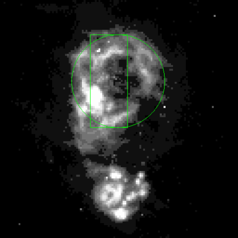
Figure 1: WFPC2 H$\alpha$ HST image of I Zw 18 aligned on NW-SE knots (WF3 image transformed to PC resolution, cf. Fig. 1 from De Mello et al. 1998; upper region: NW, lower region: SE) The circle (radius 2.5″) denotes the area used for the measurements of the H$\alpha$ and F336W flux (cf. Sect. 3.1.1, Table 2). The rectangle illustrates the aperture used for the spectroscopic observations of Izotov & Thuan (1998) centered on the NW knot. The absolute position is indicative only. F336W and F555W images indicate a small shift ($\sim$ 0.5–1 ″) between the peak emission and the center of the H$\alpha$ emission (as shown by the circle). A shift of 0.5 ″ was used for the aperture of Izotov & Thuan (1998).

As in the previous studies, we concentrate on the so-called NW component, seen in the top of Fig. 1, which shows the WFPC2 H$\alpha$ image of the HST (cf. Fig. 1 of De Mello et al. 1998). Throughout the paper, we adopt a distance to I Zw 18 of 10 Mpc, assuming $H_{o}$ = 75 km s^-1 Mpc^-1, as in many studies (Hunter & Thronson 1995, Martin 1996, van Zee et al. 1998) .

3.1.1 The stellar population

We use the same model for the stellar population as described in De Mello et al. (1998). It is provided by a evolutionary population synthesis code using stellar tracks computed with the Geneva code at the appropriate metallicity (1/50 Z_⊙). The stellar atmospheres used are spherically expanding non-LTE models for WR stars (Schmutz et al. 1992) and O stars (CoStar models at $Z=0.004$, Schaerer & de Koter 1997), and Kurucz models at [Fe/H]=-1.5 for the remainder. More details can be found in De Mello et al. (1998) and Schaerer & Vacca (1998). We assume an instantaneous burst of star formation, with an upper mass limit of 150 M_⊙ and a lower mass limit of 0.8  M_⊙. Since all observational quantities considered here depend only on the properties of massive stars, the choice for $M_{\rm low}$ has no influence for the results of this paper. It merely serves as an absolute normalisation. The total initial mass of the stars is adjusted in such a way that, at a distance of 10 Mpc, the flux at 3327 Å is equal to 1.7 10^-15  erg s^-1 cm^-2 Å^-1, the value measured in the flux calibrated WFPC2 F336W image of De Mello et al. (1998) within a circle of 2.5″ radius centered on the NW region (see Fig. 1). This flux is dominated by the latest generation of stars in I Zw 18, so that our normalization is hardly sensitive to the previous star formation history in the NW region of I Zw 18. It yields a total stellar mass of 8.7 10⁴ M_⊙, at a distance of 10 Mpc.

Actually, most of the flux comes from a region much smaller in size, and our photoionization modelling is made with the ionizing cluster located at the center of the nebula and assuming that its spatial extension is negligible.

We consider that the observed ultraviolet flux is only negligibly affected by extinction . For an extinction C(H$\beta$) of 0.04, such as estimated by Izotov & Thuan (1998), the corrected flux would be only about 10% larger, which is insignificant in our problem. Other observers give values of C(H$\beta$) ranging between 0. and 0.2. If C(H$\beta$) were as large as 0.20, as estimated by Vílchez & Iglesias-Páramo (1998) and some other observers, the true stellar flux would be a factor two higher. However, all the determinations of C(H$\beta$), except the one by Izotov & Thuan (1998), do not take into account the underlying stellar absorption at H$\beta$  and therefore overestimate the reddening. A further cause of overestimation of C(H$\beta$), which applies also to the work of Izotov & Thuan (1998), is that the intrinsic H$\alpha$/H$\beta$ ratio is assumed to be the case B recombination value, while collisional excitation of H$\alpha$ is not negligible in the case of I Zw 18 as noted by Davidson & Kinman (1985). We will come back to this below.

3.1.2 The nebula

The photoionization computations are performed with the code PHOTO using the atomic data listed in Stasińska & Leitherer (1996). The code assumes spherical geometry, with a central ionizing source. The diffuse radiation is treated assuming that all the photons are emitted outwards in a solid angle of 2$\pi$, and the transfer of the resonant photons of hydrogen and helium is computed with the same outward only approximation, but multiplying the photo-absorption cross-section by an appropriate factor to account for the increased path length due to scattering (Adams 1975).

The nebular abundances used in the computations are those we derived from the spectra of Izotov and Thuan (1998) for the NW component of I Zw 18, with the same atomic data as used in the photoionization code. For helium, however, we adopted the abundance derived by Izotov & Thuan (1998) for the SE component, as stellar absorption contaminates the neutral helium lines in the NW component. The nominal value of the temperature derived from [O iii] $\lambda$4363/5007 is 19800 K. This value was used to compute the ionic abundances of all the ions except O⁺, N⁺ and S⁺, for which a value of 15000 K was adopted (this is the typical value returned by our photoionization models for I Zw 18). The electron density deduced from [S ii] $\lambda$6731/6717 is 140 cm^-3, and this density was adopted in the computation of the ionic abundances of all species. The ionization correction factors to compute the total element abundances were those of Kingsburgh & Barlow (1994), which are based on photoionization models of planetary nebulae and are also suitable for H ii regions. They give slightly smaller oxygen abundances (by a few %) than the traditional ionization correction factors which assume that the O⁺⁺⁺ region is coextensive with the He⁺⁺ (we did not iterate on the ionization correction factors after our photoionization model analysis since this would have not changed any of the conclusions drawn in this paper). The carbon abundance used in the computations follows from the C/O ratio derived by Garnett et al. (1997) from HST observations of I Zw 18. The abundances of the elements not constrained by the observations (Mg, Si) and (Cl, Fe) have been fixed to 10^-7 and 10^-8 respectively. Table 1 presents the abundance set used in all the computations presented in the paper. As already noted by previous authors, at the metallicity of I Zw 18, the heavy elements (i.e. all the elements except hydrogen and helium) play a secondary role in the thermal balance. Their role in the absorption of ionizing photons is completely negligible. Any change of abundances, even that of helium, compatible with the observed intensities of the strong lines, will result in a very small change in the electron temperature, and we have checked that the effect they will induce in the predicted spectra are small compared to the effects discussed below.

Table 1: Input abundances relative to hydrogen for the models of I Zw 18 (by number).

He	7.60 10-2
C	3.03 10-6
N	3.89 10-7
O	1.32 10-5
Ne	2.28 10-6
S	3.72 10-7
Ar	9.13 10-8

We do not include dust in the computations. While it is known that, in general, dust mixed with the ionized gas may absorb some of the ionizing photons, and contribute to the energy balance of the gas by photoelectric heating and collisional cooling (e.g. Baldwin et al. 1991, Borkowski & Harrington 1991, Shields & Kennicutt 1995), the expected effect in I Zw 18 is negligible, since the dust-to-gas ratio is believed to be small at such metallicities (cf. Lisenfeld & Ferrara 1998).

The case of I Zw 18 is thus very interesting for photoionization modelling, since due to the very low metallicity of this object, the number of unconstrained relevant parameters is minimal.

3.2 Fitting the observational constraints

In judging the value of our photoionization models, we do not follow the common procedure of producing a table of intensities relative to H$\beta$ to be compared to the observations. A good photoionization model is not only one which reproduces the observed line ratios within the uncertainties. It must also satisfy other criteria, like being compatible with what is known from the distribution of the ionized gas, and what is known of the ionizing stars themselves. On the other hand, many line ratios are not at all indicative of the quality of a photoionization model. For example, obviously, two lines arising from the same atomic level like [O iii] $\lambda$5007 and [O iii] $\lambda$4959 have intensity ratios that depend only on the respective transition probabilities. In H ii regions, the ratio of hydrogen Balmer lines (if case B applies) is little dependent on the physical conditions in the ionized gas, and this is why it can be used to determine the reddening. The ratios of the intensities of neutral helium lines do depend somewhat on the electron density distribution and on selective absorption by dust of pseudo-resonant photons, (Clegg & Harrington 1989, Kingdon & Ferland 1995), and these are introduced in photoionization models. In the case of the NW component of I Zw 18, the observed neutral helium lines are affected by absorption from stars or interstellar sodium (Izotov & Thuan 1998, Vílchez & Iglesias-Páramo 1998), and cannot be easily used as constraints for photoionization models.

Generally speaking, once line ratios indicative of the electron temperature (like [O iii] $\lambda$4363/5007, [N ii] $\lambda$5755/6584), of the electron density (like [S ii] $\lambda$6731/6717, [Ar iv] $\lambda$4741/4713) and of the global ionization structure (like [O iii] $\lambda$5007/[O ii] $\lambda$3727 or [S iii] $\lambda$9532/[S ii] $\lambda$6725) have been fitted, the ratios of all the strong lines with respect to H$\beta$ are necessarily reproduced by a photoionization model whose input abundances were obtained from the observations. The only condition is that the atomic data to derive the abundances and to compute the models should be the same. Problems may arise only if the empirical ionization factors are different from the ones given by the model, or if there is insufficient information on the distribution of the electron temperature or density inside the nebula (in the case of I Zw 18 no direct information is available on the temperature in the low ionization zone, but we adopted a value inspired by the models). Therefore, intensity ratios such as [O iii] $\lambda$5007/H$\beta$, [Ne iii] $\lambda$3869/H$\beta$, [N ii] $\lambda$6584/H$\beta$, [Ar iii] $\lambda$7135/H$\beta$ or C iii] $\lambda$1909/H$\beta$ are not a measure of the quality of the photoionization model.

To judge whether a photoionization model is acceptable, one must work with outputs that are significantly affected by the physical processes on which the photoionization model is based, i.e. the transfer of the ionizing radiation, the processes determining the ionization equilibrium of the various atomic species and the thermal balance of the gas. Table 2 lists the quantities that can be used in the case of I Zw 18, given the observational information we have on the object. The value of the H$\beta$ flux is derived from the H$\alpha$ flux measured in a circle of radius $\theta$=2.5″ (shown in Fig. 1), assuming C(H$\beta$) = 0. The line ratios He ii $\lambda$4686/H$\beta$, [O iii] $\lambda$4363/5007, [S ii] $\lambda$6731/6717, [O iii] $\lambda$5007/[O ii] $\lambda$3727, [S iii] $\lambda$6312/[S ii] $\lambda$6725 and [O i] $\lambda$6300/H$\beta$ are the values observed by Izotov & Thuan (1998) in the rectangular aperture whose approximate position is shown in Fig. 1. It is important to define in advance the tolerance we accept for the difference between our model predictions and the observations. This must take into account both the uncertainty in the observational data, the fact that the spectra were taken through an aperture not encompassing the whole nebula, and the fact that the nebula does not have a perfect, spherical symmetric structure. This latter aspect is, of course, difficult to quantify, and the numbers given in Column 3 of Table 2 are to be regarded rather as guidelines. In Column 4, we indicate which is the dominant factor determining the adopted tolerance : the signal-to-noise, or the geometry. For example, such ratios as He ii/H$\beta$, [O iii]/[O ii], [S iii]/[S ii] or [O i]/H$\beta$ are obviously more dependent on geometrical effects than [O iii] $\lambda$4363/5007. Note that, even for that ratio, the tolerance given in Table 2 is larger than the uncertainty quoted by Izotov & Thuan (1998). The reason is that the many observations of the NW component of I Zw 18 made over the years, with different telescopes, detectors, and apertures, yield distinct values for this ratio, as shown in Fig. 2. In view of this figure, a tolerance of 10% with respect with the [O iii] $\lambda$4363/5007 ratio measured by Izotov & Thuan (1998) seems reasonable. The status of the [S ii] $\lambda$6731/6717 ratio is somewhat different. It indicates the average electron density in the zone emitting [S ii]. This is very close to an input parameter, since photoionization models are built with a given density structure. However, because the density deduced from [S ii] $\lambda$6731/6717 is not the total hydrogen density but the electron density in the region emitting [S ii], and because the density is not necessarily uniform, it is important to check that the model returns an [S ii] $\lambda$6731/6717 value that is compatible with the observations. For the total H$\beta$ flux, we accept models giving F(H$\beta$) larger than the observed value, on account of the fact that the coverage factor of the ionizing source by the nebula may be smaller than one.

Table 2: Observables that a photoionization model of I Zw 18 should fit (references in Sect. 3.2).

Quantity	Value	Tolerance	Major source of uncertainty	Symbol in Figs. 4–6
F(H$\beta$) [erg cm-2 s-1]	4.0 10-14	+ 0.5 dex	geometry (see text)	circle
angular radius $\theta$ [arc sec ]	2.5	$\pm$ 0.08 dex	geometry	cross
He ii $\lambda$4686/H$\beta$	0.034	$\pm$ 0.2 dex	geometry (see text)	square
[O iii] $\lambda$4363/5007	3.28 10-2	$\pm$ 0.04 dex	S/N	open triangle
[S ii] $\lambda$6731/6717	1.3	$\pm$ 0.04 dex	S/N	diamond
[O iii] $\lambda$5007/[O ii] $\lambda$3727	6.82	$\pm$ 0.1 dex	geometry	filled triangle
[O i] $\lambda$6300/H$\beta$	0.007	$\pm$ 0.3 dex	geometry	plus
[S iii] $\lambda$6312/[S ii] $\lambda$6725	0.173	$\pm$ 0.2 dex	geometry	asterisk

Thus, in the following, we compute photoionization models with the input parameters as defined in Section 3.1, and see how they compare with the constraints specified in Table 2. We will not examine the effects of varying the elemental abundances, since, as mentioned above, they are negligible in our problem. Uncertainties in the measured stellar flux have only a small impact on our models, and are therefore not discussed here. Similarly, we discard the effects of an error in the distance $d$ to I Zw 18. These are not crucial on the ionization structure of a model designed to fit the observed flux at 3327Å, since the mean ionization parameter varies roughly like $d^{2/3}$. What we mainly want to see is whether, with our present knowledge, we can satisfactorily explain the observed properties of I Zw 18. As will be seen, the gas density distribution plays an important role.

4 Climbing the ladder of sophistication

4.1 The ionizing radiation field

Before turning to proper photoionization modelling, it is worthwhile examining the gross properties of the ionizing radiation field of the synthetic stellar population model we are using, and compare it to single star model atmospheres. Two quantities are particularly relevant. One is $Q({\rm{He^{+}}})$/$Q({\rm{H^{0}}})$, the ratio of the number of photons above 54.4 and 13.6 eV emitted by the ionizing source. This ratio allows one to estimate the He ii $\lambda$4686/H$\beta$ that would be observed in a surrounding nebula, by using simple conservation arguments leading to the formula: He ii $\lambda$4686/H$\beta$ = 2.14 $Q({\rm{He^{+}}})$/$Q({\rm{H^{0}}})$ (taking the case B recombination coefficients given in Osterbrock 1989). As is known, this expression is valid if the nebula is ionization bounded and the observations pertain to the whole volume. It is less commonly realized that it also assumes the average temperature in the He⁺⁺ region to be the same as in the entire H ii region. This is may be far from true, as will be shown below, so a correction should account for that. Another assumption is that all the photons above 54.4 eV are absorbed by He⁺ ions. This is not what happens in objects with a low ionization parameter. There, the residual neutral hydrogen particles are sufficiently numerous to compete with He⁺. In such a case, the expression above gives an upper limit to the nebular He ii $\lambda$4686/H$\beta$ ratio. In spite of these difficulties, $Q({\rm{He^{+}}})$/$Q({\rm{H^{0}}})$ remains a useful quantity to estimate the intensity of the nebular He ii $\lambda$4686 line. Fig. 3a shows the variation of $Q({\rm{He^{+}}})$/$Q({\rm{H^{0}}})$ as a function of starburst age for the synthetic model population we are considering. As already stated in De Mello et al. (1998), the strength of the He ii nebular line in I Zw 18 indicates a starburst between 2.9 and 3.2 Myr.

Another important ratio is $Q({\rm{He^{0}}})$/$Q({\rm{H^{0}}})$, sometimes referred to as the hardness parameter of the ionizing radiation field. It provides a qualitative measure of the heating power of the stars. We have represented this quantity in Fig. 3c. We see that, as the starburst ages, its heating power gradually declines, and shows only a very mild bump at ages around 3 Myr, where the Wolf-Rayet stars are present. As we will show below this modest increase of the heating power is not sufficient to explain the high electron temperature observed in I Zw 18.

For comparison, we show in Figs. 3b and d respectively, the values of $Q({\rm{He^{+}}})$/$Q({\rm{H^{0}}})$ and $Q({\rm{He^{0}}})$/$Q({\rm{H^{0}}})$ as a function of the stellar effective temperature for the LTE model atmospheres of Kurucz (1991), the CoStar model atmospheres corresponding to main sequence stars (Schaerer & de Koter 1997) and for the model atmospheres for Wolf-Rayet stars of Schmutz et al. (1992). The CoStar models show an increased He⁺ ionizing flux compared to Kurucz models which have a negligible flux even for very low metallicities ([Fe/H]$=-1.5$). The reasons for this difference have been discussed in Schaerer & de Koter (1997). In addition to the $T_{\rm eff}$ dependence, $Q({\rm{He^{+}}})$ from WR models depend strongly on the wind density. He⁺ ionizing photons are only predicted by models with sufficiently thin winds (cf. Schmutz et al. 1992). Figure 3d shows the increase of the hardness of the radiation field, at a given $T_{\rm eff}$, between the spherically expanding non-LTE models for O and WR stars and the traditional Kurucz models (see discussion in Schaerer & de Koter 1997). This provides a greater heating power which, as will be shown later, is however still insufficient to explain the observations.

4.2 I Zw 18 as a uniform sphere

We start with the easiest and most commonly used geometry in photoionization modelling: a sphere uniformly filled with gas at constant density, occupying a fraction $\epsilon$ of the whole nebular volume. The free parameters of the models are then only the age of the starburst, the gas density and the filling factor. Each model is computed starting from the center, and the computations are stopped either when the [O iii]/[O ii] ratio has reached the observed value given in Table 2, or when the gas becomes neutral. In other words, we examine also models that are not ionization bounded, in contrast to previous studies.

Figure 4 shows our diagnostic diagram for a series of models having a density $n$= 100 cm^-3 and a filling factor $\epsilon$=0.01. The left panel shows the computed values of log F(H$\beta$) + 15 (open circles), log He ii $\lambda$4686/H$\beta$ + 2 (squares), angular radius $\theta$ (crosses), [O iii] $\lambda$4363/5007 $\times$ 100 (open triangles), [S ii] $\lambda$6731/6717 (diamonds), log ([O iii]/[O ii]) (black triangles), log ([S iii]/[S ii]) (asterisks) and log [O i]/H$\beta$ +3 (plus) as a function of the starburst age. The black circles correspond to the value of log F(H$\beta$) + 15 that the nebula would have if it were ionization bounded. Thus, by comparing the positions of an open circle and a black circle, at a given abscissa, one can immediately see whether the model is density bounded and how much diffuse H$\alpha$ or H$\beta$ emission is expected to be emitted outside the main body of the nebula. In the right panel, the observed values are represented on the same vertical scale and with the same symbols as the model predictions. The tolerances listed in Table 2 are represented as vertical error bars (the horizontal displacement of the symbols has no particular meaning). We readily see that the age of the starburst is important only for the He ii $\lambda$4686 line, the other quantities varying very little for ages 2.7–3.4 Myr. Therefore, for the following runs of models, we adopt an age of 3.1 Myr. In principle, one can always adjust the age for the model to reproduce the observed He ii $\lambda$4686/H$\beta$ ratio exactly.

Figure 5 shows the same sort of diagnostic diagram as Fig. 4 for a series of models with $n$ = 100 cm^-3 and varying filling factor. For a filling factor around 0.1 or larger, with the adopted electron density, the model is ionization bounded, and its [O iii]/[O ii] is larger than observed. For filling factors smaller than that, the gas distribution is more extended, so that the general ionization level drops. The observed [O iii]/[O ii] can then only be reproduced for a density bounded model. In such a case, the H$\beta$ radiation actually produced by the nebula is smaller than if all the ionizing photons were absorbed in the nebula. A filling factor of 0.002 – 0.05 gives values of [O iii]/[O ii], F(H$\beta$) and $\theta$ in agreement with the observations. But such models give [O iii] $\lambda$4363/5007 too small compared with the observations, and [O i]/H$\beta$ below the observed value by nearly two orders of magnitude. It is interesting, though, to understand the qualitative behavior of these line ratios as $\epsilon$ decreases. [O i]/H$\beta$ decreases because the model becomes more and more density bounded in order to reproduce the observed [O iii]/[O ii]  and levels off at $\epsilon$ = 0.1, because the ionization parameter of the model is then so small that the [O i] is gradually emitted by residual neutral oxygen in the main body of the nebula and not in the outskirts. [O iii] $\lambda$4363/5007 decreases as $\epsilon$ decreases, because of the increasing proportion of L$\alpha$ cooling as the ionization parameter drops.

One can build other series of models with different values of $n$ that are still compatible with the observed [S ii] $\lambda$6731/6717. Qualitatively, their behavior is the same and no acceptable solution is found.

Interestingly, Fig. 5 shows that models with $\epsilon$ $\geq$ 0.1 have [O iii] $\lambda$4363/5007 marginally compatible with the observations ( [O iii] $\lambda$4363/5007 = 3.03 10^-2 for $\epsilon$ = 0.1), but such models have too large [O iii]/[O ii]($>$ 10 compared of the observed value 6.8) and too small angular radius ($<$ 1.6″ instead of the observed value 2.5″). Note, by the way, that such models, being optically thick, return a rather large [O i]/H$\beta$, actually close to the observed value, and a [S iii]/[S ii] compatible with the observations. However, we do not use [S iii]/[S ii] as a primary criterion to judge the validity of a model, since experience with photoionization modelling of planetary nebulae shows that it is difficult to reproduce at the same time the sulfur and the oxygen ionization structure of a given object, and, in principle, one expects the atomic data for oxygen to be more reliable than those for sulfur. The strongest argument against models with $\epsilon>0.1$ is their angular size, which is definitely too small compared with the observations. This remains true even when considering a reasonable error on the distance since, with the condition that we impose on the flux at 3327 Å to be preserved, the angular radius of a model goes roughly like $d^{1/3}$. This illustrates the importance of taking into account other parameters in addition to line ratios to accept or reject a photoionization model.

4.3 I  Zw 18 as a spherical shell

The series of models presented above had mainly a pedagogical value, but they are obviously incompatible with the observed morphology in H$\alpha$. The next step is to consider a model consisting of a hollow, spherical shell of constant density, similar to the one constructed by García-Vargas et al. (1997) for NGC 7714 for example. In such a case, there is an additional free parameter, $R_{in}$, the radius of the inner boundary of the shell. It is fixed, more or less, by the appearance of the H$\alpha$ image. Figure 6 shows a diagnostic diagram for a series of models with $R_{in}$ = 2.25 10²⁰ cm (corresponding to an angular radius of 1.5″), $n$ = 100 cm^-3  and varying $\epsilon$. The qualitative behavior is similar to that seen for the uniform sphere models presented in Fig. 1, but the [O iii] $\lambda$4363/5007 ratio is now even lower (it never exceeds 2.5 10^-2 in this series). This is because of the enhanced role of L$\alpha$ cooling, which is strong in all the parts of the nebula, while for the full sphere model, in the zone close to the star, the ionization parameter is very high and consequently the population of neutral hydrogen very small.

Apart from the [O iii] $\lambda$4363/5007 problem, models with $\epsilon$ = 0.002 – 0.05 are satisfactory as concerns the main diagnostics ([O iii]/[O ii], F(H$\beta$) and $\theta$). The models become progressively density bounded towards smaller values of $\epsilon$ $<$ 0.02, meaning that there is a leakage of ionizing photons. From Fig. 6, one sees that these photons are enough to produce an H$\alpha$ emission in an extended diffuse envelope that is at least comparable in strength to the total emission from the dense shell. This is in agreement with Dufour & Hester’s (1990) ground-based observation of extended H$\alpha$ emission surrounding the main body of star formation.

4.4 Other geometries

Closer inspection of the HST H$\alpha$ image shows that the gas emission is incompatible with a spherical bubble. This is illustrated in Fig. 7, where the observed cumulative surface brightness profile within radius $r$ (dashed line) is compared to the expected profiles for constant density spherical shells of various inner radii (solid lines). The theoretical profiles are obtained assuming that the temperature is uniform in the gas, but taking into account a reasonable temperature gradient in the model hardly changes the picture. Clearly, the observed profile is not compatible with a spherical density distribution. The column density of emitting matter in the central zone of the image is too small. One must either have an incomplete shell with some matter stripped off from the poles, or even a more extreme morphology like an diffuse axisymmetric body with a dense ringlike equator seen face on. Such geometries are actually common among planetary nebulae (Corradi & Schwartz 1995) and nebulae surrounding luminous blue variables (Nota et al. 1995), being probably the result of the interaction of an aspherical stellar wind from the central stars (Mellema 1995, Frank et al. 1998) and are also suggested to exist in superbubbles and supergiant shells and to give rise to the blow-out phenomenon (Mac Low et al. 1989, Wang & Helfand 1991, Tenorio-Tagle et al. 1997, Oey & Smedley 1998, Martin 1998).

Does the consideration of such a geometry help in solving the [O iii] $\lambda$4363/5007 problem? In the case of a spherical shell with some matter lacking at the poles, our computations overestimate the role of the diffuse ionizing radiation, which is supposed to come from a complete shell. Since the heating power of the diffuse ionizing radiation is smaller than that of the stellar radiation, one may be underestimating the electron temperature. As a test, we have run a model switching off completely the diffuse radiation, so as to maximize the electron temperature. The effect was to increase the O⁺⁺ temperature by only 200 K. In the case of a ring with some diffuse matter seen in projection inside the ring, the gas lying close to the stars would be at a higher electron temperature than the matter of the ring, and one expects that an adequate combination of the parameters describing the gas distribution interior to and inside of the ring might reproduce the [O iii] $\lambda$4363/5007 measured in the aperture shown in Fig. 1. However, we notice that the region of high [O iii] $\lambda$4363/5007 is much larger than that. It extends over almost 20″ ( Vílchez & Iglesias-Páramo 1998) and [O iii] $\lambda$4363/5007 is neither correlated with [O iii]/[O ii] nor with the H$\alpha$ surface brightness. Therefore, one cannot explain the high [O iii] $\lambda$4363 by the emitting matter being close to the ionizing stars. In passing we note that the observations of Vílchez & Iglesias-Páramo (1998) show the nebular He ii $\lambda$4686 emission to be extended as well (although not as much as [O iii] $\lambda$4363). If this emission is due to photoionization by the central star cluster, as modelled in this paper, this means that the H$\alpha$ ring is porous, since He ii $\lambda$4686 emission necessarily comes from a region separated from the stars by only a small amount of intervening matter.

In summary, we must conclude that, if we take into account all the available information on the structure of I Zw 18, we are not able to explain the high observed [O iii] $\lambda$4363/5007 ratio with our photoionization models. In our best models, [O iii] $\lambda$4363/5007 is below the nominal value of Izotov & Thuan (1998) by 25 - 35%.

4.5 Back to the model assumptions

Can our lack of success be attributed to an improper description of the stellar radiation field? After all, we know little about the validity of stellar model atmospheres in the Lyman continuum (see discussion in Schaerer 1998). Direct measurements of the EUV flux of early B stars revealed an important EUV excess (up to $\sim$ 1.5 dex) with respect to plane parallel model atmospheres (Cassinelli et al. 1995, 1996), whose origin has been discussed by Najarro et al. (1996), Schaerer & de Koter (1997) and Aufdenberg et al. (1998). For O stars a similar excess in the total Lyman continuum output is, however, excluded from considerations of their bolometric luminosity and measurements of H ii region luminosities (Oey & Kennicutt 1997, Schaerer 1998). The hardness of the radiation field, which is crucial for the heating of the nebula, is more difficult to test. Some constraints can be obtained by comparing the line emission of nebulae surrounding hot stars with the results of photoionization models (Esteban et al. 1993, Peña et al. 1998, Crowther et al. 1999), but this is a difficult task, considering that the nebular emission depends also on its geometry. Although the hardness predicted by the CoStar O stars models permits to build grids of photoionization models that seem to explain the observations of Galactic and LMC H ii regions (Stasińska & Schaerer 1997), the constraints are not sufficient to prove or disprove the models.

To check the effect of a harder radiation field, we have run a series of models where the radiation field above 24.6 eV was arbitrarily multiplied by a factor 3 (raising the value of $Q({\rm{He^{0}}})$/$Q({\rm{H^{0}}})$ from 0.33 to 0.59, corresponding to $T_{\rm eff}$ from $\ga$ 40000 K to $\sim$ 100 000 K or a blackbody of the same temperature (cf. Fig. 3d). This drastic hardening of the radiation field resulted in an increase of [O iii] $\lambda$4363/5007 of only 10%. It is only by assuming a blackbody radiation of 300 000 K (which has $Q({\rm{He^{0}}})$/$Q({\rm{H^{0}}})$ = 0.9) that one approaches the observed [O iii] $\lambda$4363/5007. A model similar to those presented in Fig. 6 but with such a radiation field gives [O iii] $\lambda$4363/5007 =3.15 10^-2. But is has a He ii $\lambda$4686/H$\beta$ ratio of 0.53, which is completely ruled out by the observations. Of course, a blackbody is probably not the best representation for the spectral energy distribution of the radiation emitted by a very hot body, but in order to explain the emission line spectrum of I Zw 18 by stars, one has to assume an ionizing radiation strongly enhanced at energies between 20 – 54 eV, but not above 54.4 eV, compared to the model of De Mello et al. (1998). If this is realistic cannot be said at the present time.

We have also checked the effect of heating by additional X-rays that would be emitted due to the interaction of the stellar winds with ambient matter (see Martin 1996 for such X-ray observations), by simply adding a bremsstrahlung spectrum at T = 10⁶ or T = 10⁷ K to the radiation from the starburst model. As expected, the effect on [O iii] $\lambda$4363/5007 was negligible, since the X-rays are mostly absorbed in the low ionization regions (they do raise the temperature in the O⁺ zone to T_e $\simeq$ 16 000 K).

As already commented by previous authors, changing the elemental abundances does not improve the situation. Actually, even by putting all the elements heavier than helium to nearly zero abundance, [O iii] $\lambda$4363/5007 is raised by only 7%. Varying the helium abundance in reasonable limits does not change the problem.

The neglect of dust is not expected to be responsible for the too low [O iii] $\lambda$4363/5007 we find in our models for I Zw 18. Gas heating by photoemission from grains can contribute by as much as 20% to the electron thermal balance when the dust-to-gas ratio is similar to that found in the Orion nebula. But, as discussed by Baldwin et al. (1991), it is effective close to the ionizing source where dust provides most of the opacity. Besides, the proportion of dust in I Zw 18 is expected to be small, given the low metallicity. Extrapolating the relation found by Lisenfeld & Ferrara (1998) between the dust-to-gas ratio and the oxygen abundances in dwarf galaxies to the metallicity of I Zw 18 yields a dust-to-gass mass ratio 2 to 3 orders of magnitudes smaller than in the solar vicinity.

It remains to examine the ingredients of the photoionization code. We first stress that the [O iii] $\lambda$4363/5007 problem in I Zw 18 has been encountered by various authors using different codes, even if the observational material and the points of emphasis in the discussion were not the same in all the studies. As a further test, we compared the same model for I Zw 18 run by CLOUDY 90 and by PHOTO and the difference in the predicted value of [O iii] $\lambda$4363/5007 was only 5%. One must therefore incriminate something that is wrongly treated in the same way in many codes. One possibility that comes to mind is the diffuse ionizing radiation, which is treated by some kind of outward only approximation in all codes used to model I Zw 18. However, we do not expect that an accurate treatment of the diffuse ionizing radiation would solve the problem. Indeed, comparison of codes that treat more accurately the ionizing radiation with those using an outward only approximation shows only a negligible difference in the electron temperature (Ferland et al. 1996). Besides, as we have shown, even quenching the diffuse ionizing radiation does not solve the problem.

Finally, one can also question the atomic data. The most relevant ones here are those governing the emissivities of the observed [O iii] lines and the H i  collision strengths. The magnitude of the discrepancy we wish to solve would require modifications of the collision strengths or transition probabilities for [O iii] of about 25%. This is much larger than the expected uncertainties and the differences between the results of different computations for this ion (see discussion in Lennon and Burke 1994 and Galavis et al. 1997). Concerning L$\alpha$ excitation, dividing the collision strength by a factor 2 (which is far above any conceivable uncertainty, see e.g. Aggarwal et al. 1991) modifies [O iii] $\lambda$4363/5007 only by 2% because L$\alpha$ acts like a thermostat.

We are therefore left with the conclusion that the [O iii] $\lambda$4363/5007 ratio cannot be explained in the framework of photoionization models alone.

4.6 Condensations and filaments

Another failure of our photoionization models is that they predict too low [O i]/H$\beta$ compared to observations. This is a general feature of photoionization models and it is often taken as one of the reasons to invoke the presence of shocks. However, it is well known that the presence of small condensations of filaments enhances the [O i]/H$\beta$ ratio, by reducing the local ionization parameter. Another possibility is to have an intervening filament located at a large distance from the ionizing source, whose projected surface on the aperture of the observations would be small.

In order to see under what conditions such models can quantitatively account for the observed [O i]/H$\beta$ ratio, we have mimicked such a situation by computing a series of ionization bounded photoionization models for filaments of different densities located at various distances from the exciting stars. For simplicity, we assumed that there is no intervening matter between the filaments and the ionizing source. The models were actually computed for complete shells. The radiation coming from a filament can be simply obtained by multiplying the flux computed in the model by the covering factor $f$ by which the filament is covering the source.

Table 3: Line intensities relative to H$\beta$ for models of filaments.

	Main body	Filaments of various $n$			Filaments at various distances
$n$ [cm-3]	102 a	104	105	106	102	102
$\theta_{\rm in}$ [″]		1.5	1.5	1.5	20.	100.
F(H$\beta$)b	2.02e-13	3.33e-13	3.32e-13	3.35e-13	3.41e-13	3.47e-13
[O i] $\lambda$6300	1.04e-4	5.28e-2	1.57e-1	3.83e-1	6.90e-2	2.81e-1
[O ii] $\lambda$3727	2.15e-1	2.41e-1	5.39e-2	1.19e-2	4.71e-1	2.85e-1
[O iii] $\lambda$4363	3.46e-2	3.63e-5	1.12e-6	1.04e-7	1.20e-5	1.74e-7
[O iii] $\lambda$5007	1.42	3.76e-3	1.41e-4	1.25e-5	1.41e-3	3.08e-5
[S ii] $\lambda$6717	5.58e-4	5.20e-2	5.23e-2	5.27e-2	1.87e-1	5.70e-1
[S ii] $\lambda$6731.	4.19e-3	8.04e-2	9.16e-2	1.03e-1	1.35e-1	3.96e-1
a The model for the main body is density bounded (see text)
b The total H$\beta$ flux is given in erg s-1 for a covering factor $f$=1.

Table 3 presents the ratios with respect to H$\beta$ of the [O i] $\lambda$6300, [O ii] $\lambda$3727, [O iii] $\lambda$5007, [S ii] $\lambda$6717 and [S ii] $\lambda$6731 for these models. The first column of the table corresponds to a photoionization model for the main body of the nebula with $R_{in}$ = 2.25 10²⁰ cm (corresponding to $\theta_{\rm in}=$ 1.5″), $n$=100 cm^-3, and $\epsilon$=0.01, and density bounded so as to obtain the observed [O iii]/[O ii] (this is one of the models of Fig. 6). It can be readily seen that, for an intervening filament of density 10² cm^-3 located at a distance of 500 pc from the star cluster, or for condensations of density 10⁶ cm^-3, one can reproduce the observed [O i]/H$\beta$ line ratio without strongly affecting the remaining lines, not even the density sensitive [S ii] $\lambda$6731/6717 ratio, if one assumes a covering factor $f$ of about 0.1.

This explanation may appear somewhat speculative. However, one must be aware that the morphology of the ionized gas in I Zw 18 shows filaments in the main shell as well as further out and this has been amply discussed in the literature (Hunter & Thronson 1995, Dufour et al. 1995, Martin 1996). Our point is that, even in the framework of pure photoionization models, if one accounts for a density structure suggested directly by the observations, the strength of the [O i] line can be easily understood.

We note that the condensations or filaments that produce [O i]  are optically thick, and therefore their neutral counterpart should be seen in H i. Unfortunately, the available H i maps of I Zw 18 (van Zee et al. 1998) do not have sufficient spatial resolution to reveal such filaments. But these authors show that the peak emission in H i and H$\alpha$ coincide (in their paper, the peak emission in H$\alpha$ actually refers to the whole NW component), and find that the entire optical system, including the diffuse emission, is embedded in a diffuse, irregular and clumpy neutral cloud. In such a situation, it is very likely that some clumps or filaments, situated in front of the main nebula, and having a small covering factor, produce the observed [O i] line.

By using photoionization models to explain the observed [O i]/H$\beta$ ratio, one can deduce the presence of density fluctuations, even if those are not seen directly. Such density fluctuations could then be, more directly, inferred from density sensitive ratios of [Fe ii] lines, such as seen and analyzed in the Orion nebula by Bautista & Pradhan (1995).

4.7 A few properties of I Zw 18 deduced from models

Although we have not built a completely satisfactory photoionization model reproducing all the relevant observed properties of I Zw 18, we are not too far from it. We describe below some properties of the best models that may be of interest for further empirical studies of this object.

Tables 4 and 5 present the mean ionic fractions and mean ionic temperatures (as defined in Stasińska 1990) for the different elements considered, in the case of the best fit models with a uniform sphere and a spherical shell respectively, with $n$=100 cm^-3, and $\epsilon$=0.01.

It can be seen that, while both geometries yield similar ionic fractions for the main ionization stages, the relative populations of the highly charged trace ions are very different. In the case of the uniform sphere, the proportion of O⁺⁺⁺, for example, is twice as large as in the shell model. Also, the characteristic temperature of ions with high ionization potential are much higher in the case of the filled sphere, for reasons commented on earlier. As a result, the OIV]1394/H$\beta$ ratio is 9.7 10^-3 in the first case and 8.6 10^-4 in the second. This line is too weak to be measured in I Zw 18, of course, but it is useful to keep this example in mind for the study or more metal rich objects.

It is interesting to point out that, in the case of the uniform sphere, the total flux in the He ii $\lambda$4686 line is smaller than in the case of the shell model (3.1 10^-15 vs. 3.3 10^-15 erg cm^-2 s^-1) despite the fact that the ionic fractions of He⁺⁺ are similar. This is because the He⁺⁺  region is at a much higher temperature (25 000 K versus 18 000 K).

Tables 4 and 5 can be used for estimating the ionization correction factors for I Zw 18. Caution should, however, be applied regarding especially the ionization structure predicted for elements of the third row of Mendeleev’s table. Experience in photoionization modelling of planetary nebulae, where the observational constraints are larger, shows that the ionization structure of these elements is rarely satisfactorily reproduced with simple models (Howard et al. 1997, Peña et al., 1998).

The total ionized mass in the NW component is relatively well determined, since we know the total number of ionizing photons, the radius of the emitting region and have an estimate of the mean ionization parameter through the observed [O iii]/[O ii]. Indeed, at a given $Q({\rm{H^{0}}})$, for a constant density sphere with a filling factor $\epsilon$, $n^{2}\epsilon$ is proportional to the cube of the radius, while $n\epsilon^{2}$ is proportional to the cube of the ionization parameter. Of course, we have just made the point that the NW component of I Zw 18 is not a sphere. Nevertheless, we have an order of magnitude estimate, which is of 3. 10⁵ M_⊙ at $d$ = 10 Mpc (this estimate varies like $d^{3}$).

Finally, it is important to stress, as already mentioned above, that H$\alpha$ is partly excited by collisions. In all our models for the main body of the nebula, H$\alpha$/H$\beta$ lies between 2.95 and 3, while the case B recombination value is 2.7. This means that the reddening of I Zw 18 is smaller than the value obtained using the case B recombination value at the temperature derived from [O iii] $\lambda$4363/5007. If we take the observations of Izotov & Thuan (1998), who also correct for underlying stellar absorption, we obtain C(H$\beta$)=0.

5 Summary and conclusions

We have built photoionization models for the NW component of I Zw 18 using the radiation field from a starburst population synthesis at appropriate metallicity (De Mello et al. 1998) that is consistent with the Wolf-Rayet signatures seen in the spectra of I Zw 18. The aim was to see whether, with a nebular density structure compatible with recent HST images, it was possible to explain the high [O iii] $\lambda$4363/5007 ratio seen in this object, commonly interpreted as indicative of electron temperature $\simeq$ 20 000K.

For our photoionization analysis we have focused on properties which are relevant and crucial model predictions. For the observational constraints we have not only used line ratios, but also other properties such as the integrated stellar flux at 3327 Å and the observed angular radius of the emitting region as seen by the HST. Care has also been taken to include tolerances on model properties which may be affected by deviations from various simple geometries.

We have found that [O iii] $\lambda$4363/5007 cannot be explained by pure photoionization models, which yield too low an electron temperature. We have considered the effects due to departure from spherical symmetry indicated by the HST images. Indeed these show that the NW component of I Zw 18 is neither a uniform sphere nor a spherical shell, but rather a bipolar structure with a dense equatorial ring seen pole on.

We have discussed the consequences that an inaccurate description of the stellar ionizing radiation field might have on [O iii] $\lambda$4363/5007  as well as additional photoionization by X-rays. Finally, we have considered possible errors in the atomic data.

All these trials were far from solving the electron temperature problem, raising the [O iii] $\lambda$4363/5007 ratio by only a few percent while the discrepancy with the observations is on the 30% level. Such a discrepancy means that we are missing a heating source whose power may be of the same magnitude as that of the stellar ionizing photons. It is also possible that the unknown energy source is not so powerful, but acts in such a way that small quantities of gas are emitting at very high temperatures, thus boosting the [O iii] $\lambda$4363 line. Shocks are of course one of the options (Peimbert et al. 1991, Martin 1996, 1997), as well as conductive heating at the interface of an X-ray plasma with optically visible gas (Maciejewski et al. 1996). Such ideas need to be examined quantitatively, and applied to the case of I Zw 18, which we shall attempt in a future work.

What are the consequences of our failure in understanding the energy budget on the abundance determinations in I Zw 18? It depends on how the electron temperature is distributed in the O⁺⁺zone. As emphasized by Peimbert (1967, 1996) over the years (see also Mathis et al. 1998), the existence of even small zones at very high temperatures will boost the lines with high excitation threshold like [O iii] $\lambda$4363, so that the temperature derived from [O iii] $\lambda$4363/5007 will overestimate the average temperature of the regions emitting [O iii] $\lambda$5007. Consequently, the true O/H ratio will be larger than the one derived by the standard methods. The C/O ratio, on the other hand, will be smaller than derived empirically, because the ultraviolet C iii] $\lambda$1909 line will be extremely enhanced in the high temperature regions. Such a possibility was invoked by Garnett et al. (1997) to explain the high C/O found in I Zw 18 compared to other metal-poor irregular galaxies. Presently, however, too little is known both theoretically and observationally to estimate quantitatively this effect, and it is not excluded that the abundances derived so far may be correct within 30%. Obviously, high spatial resolution mapping of the [O iii] $\lambda$4363/5007 ratio in I Zw 18 would be valuable to track the origin of the high [O iii] $\lambda$4363 seen in spectra integrated over a surface of about 10 ″².

Beside demonstrating the existence of a heating problem in I Zw 18, our photoionization model analysis led to several other results.

The intensity of the nebular He ii $\lambda$4686 line can be reproduced with a detailed photoionization model having as an input the stellar radiation field that is consistent the observed Wolf-Rayet features in I Zw 18. This confirms the results of De Mello et al. (1998) based on simple Case B recombination theory.

By fitting the observed [O iii]/[O ii] ratio and the angular size of the NW component with a model where the stellar radiation flux was adjusted to the observed value, we were able to show that the H ii region is not ionization bounded and about half of the ionizing photons are leaking out of it, sufficient to explain the extended diffuse H$\alpha$ emission observed in I Zw 18.

While the [O i] emission is not reproduced in simple models, it can easily be accounted for by condensations or by intervening filaments on the line of sight. There is no need to invoke shocks to excite the [O i] line, although shocks are probably involved in the creation of the filaments, as suggested by Dopita (1997) in the context of planetary nebulae.

The intrinsic H$\alpha$/H$\beta$ ratio is significantly affected by collisional excitation: our photoionization models give a value of 3.0, to be compared to the case B recombination value of 2.75 used in most observational papers. Consequently, the reddening is smaller than usually estimated, with C(H$\beta$) practically equal to 0.

Our models can be used to give ionization correction factors appropriate for I Zw 18 for more accurate abundance determinations. However, the largest uncertainty in the abundances of C, N, O and Ne ultimately lies in the unsolved temperature problem.

It would be, of course, of great interest to find out whether other galaxies share with I Zw 18 this [O iii] $\lambda$4363/5007 problem. There are at least two other cases which would deserve a more thorough analysis. One is the starburst galaxy NGC 7714, for which published photoionization models (García-Vargas et al. 1997) also give [O iii] $\lambda$4363/5007 smaller than observed. However, it still needs to be demonstrated that this problem remains when modifying the model assumptions (e.g. the gas density distribution, possible heating of the gas by photolelectric effect on dust particles etc…). In the case of NGC 2363, the photoionization models of Luridiana et al. (1999) that were built using the oxygen abundances derived directly from the observations yielded a [O iii] $\lambda$4363/5007 ratio marginally compatible with the observations. These authors further argued that, due to the presence of large spatial temperature fluctuations, the true gas metallicity in this object is higher than derived by empirical methods. In such a case, the [O iii] $\lambda$4363/5007 ratio becomes even more discrepant.

It might well be that additional heating sources exist in giant H ii regions, giving rise to such large temperature variations and and enhancing the [O iii] $\lambda$4363 emission. As mentioned above, such a scenario needs to be worked out quantitatively.

Further detailed observational and theoretical studies of individual objects would be helpful, since we have shown that with insufficient observational constraints, high [O iii] $\lambda$4363/5007 may actually be produced by photoionization models. The effort is worthwhile, since it would have implications both on our understanding of the energetics of starburst galaxies and on our confidence in abundance derivations.

Figure 2: Observed [O iii] $\lambda$4363/5007 ratios in I Zw 18 and corresponding electron temperature. 1: Lequeux et al. (1979); 2: French (1980); 3: Kinman & Davidson (1981); 4: Davidson & Kinman (1985); 5: Dufour et al. (1988); 6, 7, 8: Pagel et al. (1992); 9: Skillman & Kennicutt (1993); 10: Stevenson et al. (1993); 11: Martin (1996); 12: Legrand et al. (1997). 13: Izotov & Thuan (1998); 14: Vílchez & Iglesias-Paramo (1998). The error bars are those quoted by the observers.

Figure 3: a) $Q({\rm{He^{+}}})$/$Q({\rm{H^{0}}})$ for starburst model at Z=0.004 from De Mello et al. (1998) as a function of age. b) $Q({\rm{He^{+}}})$/$Q({\rm{H^{0}}})$ as a function of effective temperature for different atmosphere models. SdK97: O dwarf models of Schaerer & de Koter (1997) at Z=0.004, SLG92: WR atmosphere models of Schmutz et al.  (1992). Kurucz models have negligible $Q({\rm{He^{+}}})$ values. c) Hardness parameter $Q({\rm{He^{0}}})$/$Q({\rm{H^{0}}})$ for starburst model as in a. d) $Q({\rm{He^{+}}})$/$Q({\rm{H^{0}}})$ for same atmosphere models as in b and Kurucz (1991) models for [Fe/H]=-1.5 and $\log g$=5.

Figure 4: Comparison of observed properties of I Zw 18 with a series of photoionization models of uniform spheres with $n$= 100 cm^-3 and a filling factor $\epsilon$=0.01 having, as an ionizing source, the starburst models from de Mello et al. (1998) at different ages. Left panel: models. Right panel: observations, with indication of the tolerance for the models. The following quantities are plotted: log F(H$\beta$) + 15 (open circles), log He ii $\lambda$4686/H$\beta$ + 2 (squares), angular radius $\theta$ (crosses), [O iii] $\lambda$4363/5007 $\times$ 100 (open triangles), [S ii] $\lambda$6731/6717 (diamonds), log ([O iii]/[O ii]) (black triangles), log ([S iii]/[S ii]) (asterisks) and log [O i]/H$\beta$ +3 (plus) as a function of the starburst age.

Figure 5: Same as Fig. 4 for a series of models of uniform spheres, with $n$= 100 cm^-3 and different filling factors, ionized by the radiation field from the model of de Mello et al. (1998) at an age of 3.1 Myr.

Figure 6: Same as Fig. 5 for a series of models having a shell geometry ($\theta_{in}$=1.5″).

Figure 7: Cumulative surface brightness profiles (integrated up to radius $r$) as a function of $r^{2}$ in arcsec. All profiles are normalised to $r=2.5$″. Solid lines: models for spherical shells of constant density and various inner radii. Dashed line: observed H$\alpha$ profile from the HST image shown in Fig. 1. The observations show a clear deviation from spherical gas distributions.

Table 4: Mean relative ionic abundances and mean ionic temperatures for the best uniform sphere model of Fig. 5

	I	II	III	IV	V	VI	VII	VIII	IX
H	2.585e-03	9.974e-01
	16029.	17136.
He	3.963e-03	9.658e-01	3.023e-02
	16089.	16892.	24967.
C	7.775e-05	1.074e-01	7.930e-01	9.525e-02	4.243e-03
	15846.	16168.	16947.	19230.	29282.
N	2.012e-04	1.047e-01	7.823e-01	1.115e-01	1.090e-03	1.863e-04
	15621.	15968.	16927.	19533.	28682.	35647.
O	4.044e-04	1.105e-01	8.750e-01	1.291e-02	1.126e-03	4.627e-05	6.298e-06
	15594.	15989.	17126.	26194.	31082.	36044.	40715.
Ne	4.870e-05	4.810e-02	9.367e-01	1.282e-02	2.286e-03	8.458e-05	5.971e-07
	15763.	16173.	17035.	25411.	30494.	35832.	41693.
Mg	6.431e-04	6.247e-02	8.998e-01	2.928e-02	7.267e-03	5.240e-04	1.084e-05
	16023.	16154.	16904.	23329.	27900.	32795.	38679.
Si	9.374e-05	8.091e-02	7.370e-01	1.374e-01	4.409e-02	5.123e-04
	16170.	16314.	16779.	17814.	22287.	30426.
S	3.276e-06	2.150e-02	5.415e-01	4.010e-01	3.550e-02	4.008e-04	6.938e-05
	15734.	15858.	16314.	17935.	21174.	28651.	37285.
Cl	1.374e-05	4.533e-02	5.734e-01	3.636e-01	1.670e-02	9.194e-04	3.075e-05	9.525e-06
	15835.	15938.	16396.	18119.	23487.	29260.	34968.	40585.
Ar	2.431e-06	5.553e-03	6.254e-01	3.578e-01	9.725e-03	1.437e-03	8.322e-05	3.004e-06	7.254e-07
	15517.	15865.	16329.	18257.	26182.	29982.	33949.	39752.	43983.
Fe	8.416e-06	1.722e-03	8.484e-02	8.665e-01	3.197e-02	1.204e-02	2.750e-03	2.036e-04	3.611e-06
	15512.	15518.	15860.	16894.	22399.	26289.	30082.	34962.	39424.

Table 5: Mean relative ionic abundances and mean ionic temperatures for the best spherical shell model of Fig. 6

	I	II	III	IV	V	VI	VII	VIII	IX
H	2.410e-03	9.976e-01
	16315.	16709.
He	3.938e-03	9.651e-01	3.092e-02
	16324.	16658.	18322.
C	7.507e-05	1.109e-01	8.212e-01	6.743e-02	3.274e-04
	16188.	16392.	16710.	17188.	18455.
N	1.532e-04	1.011e-01	8.224e-01	7.626e-02	1.352e-04	2.690e-07
	16013.	16271.	16714.	17216.	18287.	18819.
O	2.960e-04	1.073e-01	8.868e-01	5.670e-03	2.764e-05
	15992.	16277.	16749.	18397.	18731.
Ne	4.440e-05	5.038e-02	9.426e-01	6.959e-03	5.394e-05	0.	0.
	16110.	16381.	16714.	18208.	18616.	0.	0.
Mg	6.280e-04	6.240e-02	9.202e-01	1.652e-02	2.233e-04	4.500e-07	0.
	16285.	16371.	16705.	18116.	18547.	18831.	0.
Si	1.011e-04	7.953e-02	7.804e-01	1.244e-01	1.549e-02	1.379e-05
	16431.	16467.	16676.	16956.	17567.	18010.
S	3.123e-06	2.051e-02	5.821e-01	3.819e-01	1.545e-02	4.877e-05	2.998e-08
	16083.	16189.	16466.	17062.	17737.	18475.	19133.
Cl	1.317e-05	4.477e-02	6.190e-01	3.293e-01	6.927e-03	6.193e-05	8.940e-08	0.
	16195.	16247.	16516.	17102.	18047.	18668.	19015.	0.
Ar	1.750e-06	5.340e-03	6.789e-01	3.139e-01	1.878e-03	2.086e-05	3.481e-08
	15837.	16194.	16499.	17159.	18389.	18745.	19137.
Fe	5.725e-06	1.128e-03	7.662e-02	8.766e-01	4.300e-02	2.612e-03	3.737e-05	2.083e-08	0.
	15901.	15917.	16173.	16676.	18213.	18661.	18797.	19168.	0.