An Ongoing Parallax Microlensing Event OGLE-1999-CAR-1 Toward Carina

Abstract

We study the first microlensing event toward the Carina spiral arm discovered by the OGLE collaboration. We demonstrate that this long duration event exhibits strong parallax signatures. Additional information from the parallax effect allows us to determine the lens transverse velocity projected onto the Sun-source line to be $\sim 145\rm\,km\,s^{-1}$. We also estimate the optical depth, event rate and duration distribution for microlensing toward Carina. We show that this event is broadly consistent with these predictions.

1 Introduction

Gravitational microlensing was originally proposed as a method of detecting compact dark matter objects in the Galactic halo (Paczyński 1986). However, it also turned out to be a powerful method to study Galactic structure, mass functions of stars and extrasolar planetary systems (for a review, see Paczyński 1996). Earlier microlensing targets include the Galactic bulge, LMC, SMC and M31. Recently, the EROS and OGLE collaborations have started to monitor spiral arms. The EROS collaboration (Derue et al. 1999) has announced the discovery of three microlensing events toward two spiral arms. In this paper, we study the first spiral arm microlensing event discovered by the OGLE II experiment (Udalski, Kubiak & Szymański 1997). This ongoing event, OGLE-1999-CAR-1, was discovered in real-time toward the Carina arm by the OGLE early-warning system (Udalski et al. 1994). We show that this is a unique event that exhibits strong parallax effects. Such events were predicted by Refsdal (1966) and Gould (1992). The first case was reported by the MACHO collaboration toward the Galactic bulge (Alcock et al. 1995). OGLE-1999-CAR-1 is the first parallax event discovered toward any spiral arm. The outline of the paper is as follows. In Sect. 2, we briefly describe the observational data that we use. In Sect. 3, we present two different fits for the light curve, with and without considering the effect of parallax and blending. In Sect. 4, we calculate the expected optical depth, event rate and duration distribution toward Carina. Finally in Sect. 5, we summarize and discuss the implications of our results.

2 Observational Data

The observational data were collected by the OGLE collaboration in their second phase of microlensing search (Udalski et al. 1997). The search was done with the 1.3-m Warsaw telescope at the Las Campanas Observatory, Chile which is operated by the Carnegie Institution of Washington. The targets of the OGLE II experiment include the LMC, SMC, Galactic bulge and spiral arms. All the collected data were reduced and calibrated to the standard system. For more details on the instrumentation setup and data reduction, see Udalski et al. (1997, 1998).

The event, OGLE-1999-CAR-1, was detected and announced in real-time on Feb. 19, 1999 by the OGLE collaboration . Its equatorial coordinates are $\alpha$=11:07:26.72, $\delta$=-61:22:30.6 (J2000), which corresponds to Galactic coordinates $l=290^{\circ}.8,b=-0^{\circ}.98$. The ecliptic coordinates of the lensed star are $\lambda=331^{\circ}.9$, $\beta=-58^{\circ}.1$ (e.g., Lang 1980). Finding chart and I-band data of OGLE-1999-CAR-1 are available at the above web site and the V-band data were made available to us by Dr. Andrzej Udalski. In total, there are 416 I-band and 85 V-band data points. The baseline magnitudes of the object , in the standard Johnson V and Cousins I-band, are $V=19.66,I=18.01$.

3 Models

In this section, we will fit the OGLE V and I-band light curves simultaneously with theoretical models. We start with the simple standard model, and then consider a fit that takes into account both parallax and blending.

Most microlensing light curves are well described by the standard form (e.g., Paczyński 1986):

$$A(t)={u^{2}+2\over u\sqrt{u^{2}+4}},\leavevmode\nobreak\ \leavevmode\nobreak\ u(t)\equiv\sqrt{u_{0}^{2}+w^{2}(t)},$$ (1)

where $u_{0}$ is the impact parameter (in units of the Einstein radius) and

$$w(t)={t-t_{0}\over t_{E}},\leavevmode\nobreak\ \leavevmode\nobreak\ t_{E}\equiv R_{E}/v_{t}$$ (2)

with $t_{0}$ being the time of the closest approach (maximum magnification), $R_{E}$ the Einstein radius, $v_{t}$ the lens transverse velocity relative to the observer-source line of sight, and $t_{E}$ the Einstein radius crossing time. The Einstein radius is defined as

$$R_{E}=\sqrt{4GMD_{\rm s}x(1-x)\over c^{2}},$$ (3)

where $M$ is the lens mass, $D_{\rm s}$ the distance to the source and $x=D_{\rm d}/D_{\rm s}$ is the ratio of the distance to the lens and the distance to the source.

To fit both the I-band and V-band data with the standard model, we need five parameters, namely,

$$u_{0},t_{0},t_{E},m_{\rm I,0},m_{\rm V,0}.$$ (4)

Best-fit parameters are found by minimizing the usual $\chi^{2}$ using the MINUIT program in the CERN library and are tabulated in Table 1. The resulting $\chi^{2}$ is 893.9 for 496 degrees of freedom. For convenience, we divide the data into one ‘unlensed’ part and one ‘lensed’ part; the former has $t={\rm J.D.}-2450000<1150\thinspace{\rm d}$ and the latter has $t>1150\thinspace{\rm d}$. For the standard fit, the lensed part has $\chi^{2}=407.9$ for 161 data points, and the unlensed part has $\chi^{2}=486.0$ for 340 data points; the somewhat high $\chi^{2}$ for this part may be due to contaminations of nearby bright stars (as can be seen in the finding chart), particularly at poor seeing conditions. The $\chi^{2}$ per degree of freedom for the ‘lensed’ part is about 2.5, indicating that the fit is not satisfactory. This can also be seen from Fig. 1, where we show the model light curve together with the data points. As can be seen, the observed values are consistently brighter than the predicted ones for $t>1325\thinspace{\rm d}$ in the I-band. Further, the prediction is fainter by about 0.05 magnitude at the peak in the V-band. We show next that both inconsistencies can be removed by incorporating parallax effect and blending.

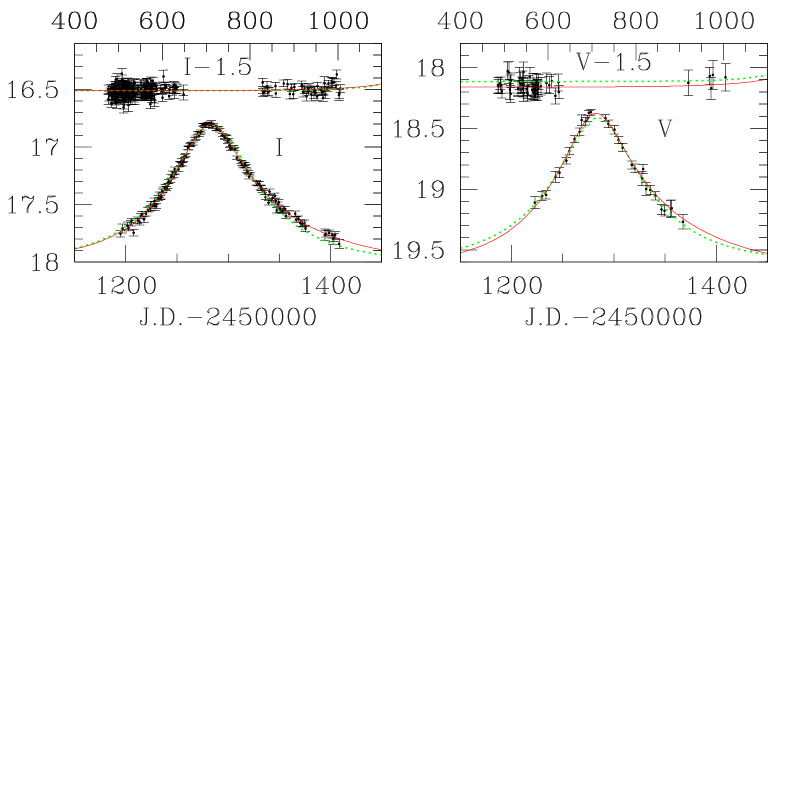
Figure 1: The I-band (left) and V-band (right) light curves observed by the OGLE collaboration are shown. In each panel, the constant part of light curve is shown at the top with their amplitudes shifted by 1.5 magnitude and with their time intervals (from $400\thinspace{\rm d}$ to $1100\thinspace{\rm d}$) labelled at the top axis. The dotted line indicates the best-fit standard model (eq. 1), while the solid line is for the best-fit model that takes into account both parallax (eq. 5) and blending (eq. 9). Fit parameters are given in Table 1.

Table 1: The best standard model (first row) and the best parallax model with blending (second row) for OGLE-1999-CAR-1.

	$t_{0}$	$t_{E}$	$u_{0}$	$m_{\rm I,0}$	$m_{\rm V,0}$	$\theta$	$\tilde{v}$	$f_{I}$	$f_{V}$	$\chi^{2}$
S	$1284.2^{+0.1}_{-0.1}$	$89.8^{+0.45}_{-0.45}$	$0.35^{+0.01}_{-0.01}$	$18.01^{+0.02}_{-0.02}$	$19.62^{+0.05}_{-0.05}$	—	—	—	—	893.9
P	$1288.8^{+1.7}_{-1.6}$	$118.1^{+10.8}_{-6.9}$	$0.24^{+0.05}_{-0.03}$	$18.01^{+0.02}_{-0.02}$	$19.66^{+0.09}_{-0.09}$	$-0.94^{+0.75}_{-0.73}$	$145.5^{+13.0}_{-40.8}$	$0.36^{+0.2}_{-0.2}$	$0.29^{+0.2}_{-0.2}$	640.9

To take into account the Earth motion around the Sun, we have to modify the expression for $u(t)$ in eq. (1). This modification, to the first order of the Earth’s orbital eccentricity ($\epsilon=0.017$), is given by Alcock et al. (1995) and Dominik (1998):

$$u^{2}(t) = u_{0}^{2}+w(t)^{2}+\tilde{r}_{\oplus}^{2}\sin^{2}\psi$$ (5)

$$+ 2\tilde{r}_{\oplus}\sin\psi\left[w(t)\sin\theta+u_{0}\cos\theta\right]+\tilde{r}_{\oplus}^{2}\sin^{2}\beta\cos^{2}\psi$$

$$+ 2\tilde{r}_{\oplus}\sin\beta\cos\psi\left[w(t)\cos\theta-u_{0}\sin\theta\right],$$

where $\theta$ is the angle between $\@vec{v}_{t}$ and the line formed by the north ecliptic axis projected onto the lens plane, $u_{0}$ is now more appropriately the minimum distance between the lens and the Sun-source line. The expression of $\tilde{r}_{\oplus}$ and $\psi$ are given by

$$\tilde{r}_{\oplus}={1{\rm AU}\over\tilde{v}\leavevmode\nobreak\ t_{E}}\{1-\epsilon\cos[\Omega_{0}(t-t_{p})]\},$$ (6)

and

$$\psi=-\phi+\Omega_{0}(t-t_{p})+2\epsilon\sin[\Omega_{0}(t-t_{p})],$$ (7)

where $t_{p}$ is the time of perihelion, $\tilde{v}=v_{t}/(1-x)$ is the transverse speed of the lens projected to the solar position, $\Omega_{0}=2\pi/{\rm yr}$, and $\phi$ is the longitude measured in the ecliptic plane from the perihelion toward the Earth’s motion; this is given in the appendix of Dominik (1998),

$$\phi=\lambda+\pi+\phi_{\gamma},$$ (8)

where $\phi_{\gamma}$ is the longitude of the vernal equinox measured from the perihelion. $\phi_{\gamma}=1.33$ (rad), and the Julian day for Perihelion is $t_{p}=2451181.57$; the readers are referred to the The Astronomical Almanac (1999) for the relevant data. Note that the inclusion of the parallax effect introduces two more parameters, $\tilde{v}$ and $\theta$.

The two-color light curves show that the lensed object became bluer by $\approx 0.05$ mag at the peak of magnification; such chromaticity is easily produced by blending. The additional source of light may be from the lens itself and/or it can come from another star which lies in the seeing disk of the lensed star by chance alignment. When blending is present, the observed magnification is given by

$$A_{i}=f_{i}+(1-f_{i})A(t),\leavevmode\nobreak\ \leavevmode\nobreak\ i=I,V.$$ (9)

To model the blending in two colors, we need two further parameters – the fraction of light contributed by the unlensed component in I and V, $f_{I}$ and $f_{V}$, at the baseline. Therefore, a fit that takes into account both parallax and blending effects requires 9 parameters: $u_{0},t_{0},t_{E},m_{\rm I,0}$, $m_{\rm V,0}$, $\tilde{v},\theta,f_{I}$, and $f_{V}$.

The best-fit parameters for this model are given in Table 1. Compared with the standard fit, the $\chi^{2}$ is reduced from 893.9 to 640.8. The reduction in the lensed part is dramatic: the $\chi^{2}$ drops from 407.9 to 177.7 for 161 data points. The $\chi^{2}$ for the unlensed part is 463.2 (as compared to 486.0 for the standard fit) for 340 data points. The $\chi^{2}$ per degree of freedom is satisfactory. The predicted light curve (solid line in Fig. 1) matches the observed data both in the I-band and V-band. From Table 1, the blending fractions in the V and I bands are not well constrained, $f_{I}=0.36\pm 0.2$ and $f_{V}=0.29\pm 0.2$. The differential blending, however, is reasonably constrained, $f_{V}/f_{I}=0.81^{+0.1}_{-0.27}$ due to the observed differential magnification (0.05 mag) between the I-band and V-band. The projected lens velocity is well constrained while its direction has somewhat larger errors. For completeness, we mention that the best model that accounts for blending but not parallax has $\chi^{2}=791.8$ while the best model that accounts for parallax but not blending has $\chi^{2}=682.2$. Hence the parallax effect reduces the $\chi^{2}$ much more effectively than blending. This can be easily understood since the observed light curve is asymmetric, which cannot be produced by blending.

4 Optical Depth and Event Rate Toward Carina

To put OGLE-1999-CAR-1 into context, in this section we estimate the optical depth, event rate and event duration distribution toward Carina. These can be compared with future observations when more events become available.

One major uncertainty for microlensing toward spiral arms such as Carina is that we do not know the distance to the sources. Several molecular clouds at the same direction have distances between $6.8\,{\rm{kpc}}$ and $8.7\,{\rm{kpc}}$ (see Table 1 and Fig. 4. in Grabelsky et al. 1988). We adopt $D_{\rm s}=6.8\,{\rm{kpc}}$ as the distance to the sources. This assumption is also consistent with the lensed star being a main-sequence star as required by its position in the color-magnitude diagram (Udalski 1999, private communication); we return to this issue in the discussion.

Since the direction toward the lensed star is nearly in the Galactic plane ($b=-0^{\circ}.98$) and far away from the Galactic center, we assume that the lenses are entirely contributed by disk stars, and their density profile follows the standard double exponential disk distribution

$$\rho(R,z)={\Sigma\over 2z_{0}}\leavevmode\nobreak\ \exp\left(-{r-r_{0}\over r_{d}}\right)\exp\left(-{|z|\over z_{0}}\right),$$ (10)

where $\Sigma=50M_{\odot}/{\rm pc}^{2}$, $r$ is the lens distance to the Galactic center, $r_{0}=8.5\,{\rm{kpc}}$, disk scale-length $r_{d}=3.5\,{\rm{kpc}}$ and scale-height $z_{0}=0.325\,{\rm{kpc}}$. The optical depth can then be obtained (e.g., eq. 9 in Paczyński 1986):

$$\tau=3.4\times 10^{-7},$$ (11)

independent of the lens mass function and kinematics.

Figure 2: The left panel shows the predicted event rate distribution (in units of per million stars per year) as a function of duration toward Carina. The short dashed line is for a $\delta$-mass function of $1M_{\odot}$, the long dashed line is for a Salpeter mass function, $n(M)dM\propto M^{-2.35}dM$ and the solid line is for a disk mass function, $n(M)dM\propto M^{-0.54}dM$, determined from HST star counts. The shaded region indicates the $1\sigma$ range in time-scale for the best parallax fit with blending. The right panel shows the likelihood function and lens mass as a function of the lens distance, respectively.

To estimate the event rate and event duration distribution, we have to make assumptions about the lens kinematics and mass function. The motion of lenses can be divided into an overall Galactic rotation of $220\rm\,km\,s^{-1}$ and a random motion. We assume that the random component follows Gaussian distributions with velocity dispersions of $\sigma_{R}=40\rm\,km\,s^{-1},\sigma_{\theta}=30\rm\,km\,s^{-1},\sigma_{z}=20\rm\,km\,s^{-1}$ (cf. Derue et al. 1999). The motion of the Sun relative to the Local Standard of Rest is taken as $v_{R,\odot}=9\rm\,km\,s^{-1},v_{\theta,\odot}=11\rm\,km\,s^{-1},v_{z,\odot}=16\rm\,km\,s^{-1}$. We study three mass functions:

1. $n(M)dM\propto\delta(M-1M_{\odot})dM$,

2. $n(M)dM\propto M^{-2.35}dM,\leavevmode\nobreak\ \leavevmode\nobreak\ 0.08M_{\odot}<M<1M_{\odot}$,

3. $n(M)dM\propto M^{-0.54}dM,\leavevmode\nobreak\ \leavevmode\nobreak\ 0.1M_{\odot}<M<0.6M_{\odot}$.

Note that the second is a Salpeter mass function while the third describes the local disk mass function determined using HST star counts (Gould et al. 1997). The predicted event duration distributions for these three mass functions are shown in the left panel of Fig. 2. It is clear that there is a tail toward long durations for all three distributions. The probabilities of having $t_{E}$ longer than $100\thinspace{\rm d}$ are respectively, $\sim$ 50%, 10% and 20%; so the observed long duration is not statistically rare. The total event rates per million stars per year are found to be

$$\Gamma=0.64,1.4,1.1,$$ (12)

for the three mass functions, respectively. The predicted duration distribution and event rate are sensitive to the assumed velocity dispersions. For example, if we adopt $\sigma_{R}=\sigma_{\theta}=\sigma_{z}=20\rm\,km\,s^{-1}$ (as in Kiraga & Paczyński 1994), then the events will be on average 30% longer and the event rate decreases by about 30%.

5 Discussion

We have shown that the microlensing event, OGLE-1999-CAR-1, has a light curve shape that is significantly modified by the earth motion around the Sun. This event is still ongoing at the time of writing (Aug. 12, 1999); later evolutions of the light curve will test our predictions and reduce the uncertainties in the parameters. For comparison, the three microlensing events seen by the EROS collaboration (Derue et al. 1999) are toward different spiral arms which are somewhat closer to the Galactic center direction. The three events have $t_{E}$ between 70$\thinspace{\rm d}$ to 100$\thinspace{\rm d}$, and none of the events show parallax effects.

We have assumed a source distance of $6.8\,{\rm{kpc}}$ in the previous section. We show now that this is a reasonable assumption. From $V=19.66$ and $I=18.01$, and taking into account the blending, we find that the lensed star has $M_{V}=5.9,M_{I}=4.3$. Assuming an extinction of $A_{V}=1.5$ mag (see Fig. 4 in Wramdemark 1980), and $A_{I}/A_{V}=0.482$, we obtain the intrinsic magnitude and color $M_{V}=4.4,(V-I)_{0}=0.75$. The star is consistent with being a main sequence star (with mass $M\sim 1.05M_{\odot}$), as can be seen from the color-magnitude diagram (Udalski 1999, private communication) in the Carina region.

We can combine the expression for $\tilde{v}$ and $t_{E}$ to obtain the lens mass as a function of its distance

$$M={1-x\over x}{\tilde{v}^{2}t_{E}^{2}c^{2}\over 4GD_{\rm s}}\approx 1.8M_{\odot}{1-x\over x}.$$ (13)

Using eq. (6) in Alcock et al. (1995), we have calculated the likelihood of obtaining the observed transverse velocity and direction as a function of the lens distance. The result is shown in the right panel of Fig. 2 for the Gould et al. (1997) mass function. The lens distance is approximately $x=0.5\pm 0.2$; we caution that this likelihood function is sensitive to the assumed kinematics. For example, if we take $\sigma_{R}=\sigma_{\theta}=\sigma_{z}=20\rm\,km\,s^{-1}$, then the best-fit lens distance changes to $x=0.7$. It is possible that a lens is a (massive) dark lens such as a white dwarf, neutron star and black hole; in this case the blended light is contributed by another unrelated star. Another possibility is that the blending is contributed by the lens itself. If the lens is a main sequence star and $x\approx 0.7$, which implies $M\approx 0.8M_{\odot}$, then the lens will contribute about the right amount of light to explain the light curves (including the color change in the V and I bands). Further high-resolution imaging of the lensed object should allow us to differentiate between these two possibilities.

- (1) Alcock C, Allsman R.A., Alves D. et al., 1995, ApJ 454, L125
- (2) Derue F., Afonso C., Alard C. et al., 1999, preprint (astro-ph/9903209)
- (3) Dominik M., 1998, A&A 329, 361
- (4) Grabelsky D. A., Cohen R. S., Bronfman L., Thaddeus P., 1988, ApJ 331, 181
- (5) Gould A., 1992, ApJ 392, 442
- (6) Gould A., Bahcall J. N., Flynn C., 1997, ApJ 482, 913
- (7) Kiraga M., Paczyński B., 1994, ApJ 430, L101
- (8) Lang K. R., 1980, Astrophysical Formulae (Springer-Verlag: Berlin), 504
- (9) Paczyński B., 1986, ApJ 304, 1
- (10) Paczyński B., 1996, ARA&A 34, 419
- (11) Refsdal S., 1966, MNRAS 134, 315
- (12) Udalski A., Kubiak M., Szymański M., 1997, Acta Astron. 47, 319
- (13) Udalski A., Szymański M., Kaluzny J. et al., 1994, Acta Astron. 44, 227.
- (14) Udalski A., Szymański M., Kubiak M. et al., 1998, Acta Astron. 48, 147
- (15) Wramdemark S., 1976, A&AS 23, 231