The Hubble Constant and the Expansion Age of the Universe

Abstract

The Hubble constant, which measures the expansion rate, together with the total energy density of the Universe, sets the size of the observable Universe, its age, and its radius of curvature. Excellent progress has been made recently toward the measurement of the Hubble constant: a number of different methods for measuring distances have been developed and refined, and a primary project of the Hubble Space Telescope has been the accurate calibration of this difficult-to-measure parameter. The recent progress in these measurements is summarized, and areas where further work is needed are discussed. Currently, for a wide range of possible cosmological models, the Universe appears to have a kinematic age less than about 14$\pm$2 billion years. Combined with current estimates of stellar ages, the results favor a low–matter–density universe. They are consistent with either an open universe, or a flat universe with a non-zero value of the cosmological constant.

    THE HUBBLE CONSTANT

AND THE EXPANSION AGE OF THE UNIVERSE

   Wendy L. Freedman¹

¹ Carnegie Observatories, 813 Santa Barbara St., Pasadena, CA 91101.

To be published in the David Schramm Memorial Volume, Physics Reports, Elsevier, 2000, in press.

1 Introduction

The Hubble constant (H₀) is one of the most important parameters in Big Bang cosmology: the square of the Hubble constant relates the total energy density of the Universe to its geometry kt ; pea . H₀ enters in a practical way into many cosmological and other astrophysical calculations: together with the energy density of the Universe, it sets the age of the Universe, t, the size of the observable Universe (R_obs = ct), and its radius of curvature ($R_{curv}={c\over H_{0}}{{(\Omega-1)}\over k}^{-{1\over 2}}$). The density of light elements (H, D, ³He, ⁴He and Li) synthesized after the Big Bang also depends on the expansion rate. These limits on the density of baryonic matter can then be used to set limits on the amount of non-baryonic matter in the Universe. The determination of numerous physical properties of galaxies and quasars (mass, luminosity, energy density) all require knowledge of the Hubble constant.

Primarily as a result of new instrumentation at ground-based telescopes, and most recently with the successful refurbishment of the Hubble Space Telescope (HST), the extragalactic distance scale field has been evolving at a rapid pace. Still, until very recently, a factor-of-two uncertainty in the value of H₀ has persisted for a variety of reasons jacoby92 ; wlfprinceton . Since the 1980’s, linear detectors, replacing photographic plates, have enabled much higher accuracy measurements, corrections for the effects of dust, and measurements to much greater distances, all combining to increase the precision in the relative distances to galaxies. Prior to HST, however, very few galaxies were close enough to allow the discovery of Cepheid variables, upon which the absolute calibration of the extragalactic distance scale largely rests mf91 ; fmtrimble .

In the following sections I summarize how the Hubble constant is measured in practice, and the problems encountered in doing so. I describe in general how to measure distances, list both the strengths and weaknesses of various methods for measuring distances, and then discuss the factors that affect the determination of true, expansion velocities. In addition, I briefly review the method, the results and the uncertainties for the determination Cepheid distances to galaxies, and recent results from the Hubble Space Telescope (HST) by the H₀ Key Project and other groups. I then give the implications of these results for cosmology, and compare these “local” results to methods that can be applied directly at high redshifts. Finally, I highlight areas where future work would be profitable.

2 Measuring the Hubble Constant

Determination of the Hubble constant is extremely simple in principle: measure the recession velocities and the distances to galaxies at sufficiently large distances where deviations from the smooth Hubble expansion are small, and the Hubble constant follows immediately from the slope of the correlation between velocity and distance. However, progress in measuring H₀ has been limited by the fact that there exist few methods for measuring distances that satisfy many basic criteria. Ideally, a distance indicator should be based upon well-understood physics, operate well out into the smooth Hubble flow (velocity-distances greater than $\sim$10,000 km/sec), be applied to a statistically significant sample of objects, be empirically established to have high internal accuracy, and most importantly, be demonstrated empirically to be free of systematic errors. The above list of criteria applies equally well to classical distance indicators as to other physical methods (in the latter case, for example, the Sunyaev Zel’dovich effect or gravitational lenses).

Historically, measuring accurate extragalactic distances has been enormously difficult; in retrospect, the difficulties have been underestimated and systematic errors have dominated. And still today, the critical remaining issue is to identify and reduce any remaining sources of systematic error. At the present time, an ideal distance indicator or other method meeting all of the above criteria does not exist, and measurement of H₀ as high as 1$\%$ accuracy is clearly a goal for the future. However, as described below, an accuracy of H₀ to 10% has now likely been reached.

3 Recession Velocities

Since the velocity of recession of a galaxy is proportional to its distance (Hubble’s law), the farther that distance measurements can be made, the smaller the proportional impact of peculiar motions on the expansion velocities. For a galaxy or cluster at a recession velocity of 10,000 km/sec, the impact of a peculiar motion of 300 km/sec giovanelli98 is 3% on H₀ for that object. This uncertainty is reduced by observing a number of objects, well-distributed over the sky, so that such motions can be averaged out. Moreover, given the overall mass distribution locally, a correction for peculiar motions can be applied to the velocities (over and above corrections for the Earth’s, Sun and our Milky Way’s motion in the Local Group). For type Ia supernovae, the distant indicator which currently extends the farthest (v $\sim$ 30,000 km/sec), the effects of peculiar motions are a small fraction of the overall error budget.

4 Distances to Galaxies

In astronomy most length scales cannot be measured directly – the size scales, especially in a cosmological context are too vast. Direct trigonometric parallaxes (using the Earth’s orbit as a baseline for triangulation) can be measured for the nearest stars in our Milky Way galaxy, but this technique currently can be applied reliably only for relatively nearby stars within our own Galaxy. More distant stars in our Galaxy and then extragalactic objects require other, more indirect indicators of distance.

In general, the most common means for estimating extragalactic distances make use of the inverse square radiation law. If objects can be identified whose luminosities are either constant (“standard candles”), or perhaps related to a quantity that is independent of distance (for example, period of oscillation, rotation rate, velocity dispersion, or color) then given an absolute calibration, their distances can be gauged. The “standard candles” must be independently calibrated to absolute physical units so that true distances (in units of megaparsecs, where 1 Mpc = 3.09 $\times$ 10²² m) can be determined. Ultimately, these calibrations tie back to geometric parallax distances. Alternatively a “standard ruler” can be used, making use of the fact that physical dimensions scale inversely as the distance. Several methods for measuring distances to galaxies are summarized below.

4.1 Cepheid variables

Primary amongst the distance indicators are the Cepheid variables, stars whose outer atmospheres pulsate regularly with periods ranging from 2 to about 100 days. Cepheids are bright, young stars, abundant in nearby spiral and irregular galaxies. The underlying physics of the pulsation mechanism is simple and has been studied extensively cox . Empirically it has been established that the period of pulsation (a quantity independent of distance) is very well correlated with the intrinsic luminosity of the star. The dispersion in the Cepheid period-luminosity relation in the I band ($\sim$8000 Angstroms) amounts to about 20% in luminosity. From the inverse square law, this corresponds to an uncertainty of about 10% in the distance for a single Cepheid. With a sample of 25 Cepheids in a galaxy, a statistical uncertainty of about 2% in distance can be achieved. Hence, Cepheids provide an excellent means of estimating distances to resolved spiral galaxies. I return in §§4.7, 5.2 and 6.1 to a discussion of the largest remaining uncertainties in the Cepheid distance scale.

The reach of Cepheid variables as distance indicators is limited. With available instrumentation, for distances beyond 20 Mpc or so, brighter objects than ordinary stars are required; for example, measurements of luminous supernovae or the luminosities of entire galaxies. Implementation of these secondary methods are now briefly described in turn.

4.2 Type Ia Supernovae

Perhaps the most promising of the cosmological distance indicators are the luminous supernovae classified as type Ia. Type Ia supernovae show no hydrogen in their spectra, and are believed to result from the explosion of a carbon-oxygen white dwarf which burns into ⁵⁶Ni. livio . These objects have luminosities comparable to entire galaxies of moderate luminosity, and hence can be observed to distances of hundreds of Mpc tammsand ; hamuy96 ; rpk . They have a narrow range in maximum luminosity and empirically an additional relation exists between the luminosity of the supernova at its maximum and the rate at which the supernovae subsequently decreases in brightness, phil ; rpk . Bright supernovae decline more slowly. Using this correlation, the dispersion for type Ia supernovae drops to about 12% in luminosity, corresponding to an uncertainty of about 6% in the distance for a single supernova rpk . Currently no other secondary distance indicator rivals this precision. Unfortunately, the exact mechanism for the ignition of the explosion has not yet been theoretically or observationally established, nor are the progenitors known with any certainty. Ultimately, confidence in this empirically-based method will be strengthened as the theoretical basis is more firmly established.

4.3 The Tully–Fisher relation

For spiral galaxies, the total (face–on) luminosity shows an excellent correlation with the maximum rotation velocity of the galaxy tf ; ahm ; pt ; giovanelli97 . This relationship reflects the fact that more massive (and luminous) galaxies must rotate more rapidly to rotationally support themselves. Independent of distance, galaxy rotation rates can be measured spectroscopically (from Doppler shifts of spectral features of hydrogen at radio or optical wavelengths). This relation has been measured for hundreds of galaxies within clusters, and in the general field. Empirically, it has been established that the dispersion in this relation amounts to about 30% in luminosity, or a 15% distance uncertainty for an individual galaxy. By measuring a couple of dozen or more galaxies in a single cluster, the statistical uncertainty in distance can be reduced to a few percent.

4.4 Fundamental Plane

For elliptical galaxies, a correlation between the stellar velocity dispersion and the intrinsic luminosity exists, analogous to the relation between rotation velocity and luminosity for spirals fj . Elliptical galaxies also occupy a ‘fundamental plane’ wherein the galaxy size is tightly correlated with the surface brightness and velocity dispersion of the galaxy 7S ; djor ; jorgen96 . The scatter in this relation is only 10–20% in distance. Both the Tully-Fisher and fundamental plane relations will be limited in precision as distance indicators to the extent that the mass–to–light ratios of galaxies are not universal and that star formation histories may vary (that is, the stellar populations within galaxies have different mean ages or chemical compositions for a given mass). Empirically, however, with few exceptions, deviations from these relations are measured to be very small, providing compelling evidence that mass–to–light and stellar population variations are quantitatively constrained by the scatter in the observed relations giovanelli98 ; jorgen96 .

4.5 Surface Brightness Fluctuations

Another method with high internal precision, developed by Tonry and Schneider ts , makes use of the fact that the resolution of stars within galaxies is distance dependent. In each pixel on a CCD detector, a given number of stars contributes to the luminosity. The Poisson fluctuations from pixel to pixel then depend on the distance to the galaxy. They have been empirically determined to be a strong function of the color of the stars. Once other sources of noise (bad pixels on the detector, objects such as star clusters, background galaxies, foreground stars) have been removed, by normalizing to the average flux, this method provides a means of measuring relative distances to galaxies that has been established empirically to yield a precision of $\sim$8% tonry97 . With HST, this method is now being applied out to velocities of about 5,000 km/sec lauer98 ; tonry97 . This method is applied to elliptical galaxies or to spirals with prominent bulges.

4.6 From Relative to Absolute Distances

The secondary methods described above (type Ia supernovae, the Tully-Fisher relation, the fundamental plane, and surface brightness fluctuations) provide several means of measuring relative distances to galaxies. The absolute calibration for all of these methods is presently established using the Cepheid distance scale. To give a specific example, absolute distances for supernovae require both measurements of the apparent luminosities of distant supernovae (the quantity observed), as well as distances to nearby galaxies in which type Ia supernovae have also been observed. The distances to nearby type Ia supernovae galaxy hosts are needed to provide the absolute luminosities of supernovae. Only then can an absolute distance scale be set for the more distant supernovae. Although references are occasionally made to the “Cepheid distance scale” and the “supernova distance scale”, the supernova distance scale is not independent of, but is built upon, the Cepheid distance scale. With the exception of theoretical models of supernovae, all H₀ measurements of supernovae are calibrated using the Cepheid distance scale. The same holds true for all of the other methods listed above.

4.7 Systematic Effects in Distance Measurements

Many distance indicators have sufficiently small scatter that with the current numbers of Cepheid calibrators, the statistical precision in their distance scales is 5% or better. The total uncertainty associated with the measurement of distances is higher, however, because of complications due to other astrophysical effects. Many of these systematic effects are common to all of these measurements, although their cumulative impact may vary from method to method.

Dust grains in the regions between stars, both within our own Galaxy and in external galaxies, scatter blue light more than red light, with a roughly 1/$\lambda$ dependence. The consequences of this interstellar dust are two-fold: 1) objects become redder (a phenomenon referred to as reddening) and 2) objects become fainter (commonly called extinction). If no correction is made for dust, objects appear fainter (and therefore apparently farther) than they actually are. Since the effects of dust are wavelength dependent, corrections for reddening and extinction can be made if observations are made at two or more wavelengths wlf1613 ; mf91 ; rpk ; tonry97 .

A second potential systematic effect is that due to chemical composition or metallicity. Stars have a range of metallicities, depending on the amount of processing by previous generations of stars that the gas (from which they formed) has undergone. In general, older stars have lower metallicities, although there is considerable dispersion at any given age. Metals in the atmospheres of stars act as an opacity source to the radiation emerging from the nuclear burning. These metals absorb primarily in the blue part of the spectrum, and the radiation is thermally redistributed and primarily re-emitted at longer (redder) wavelengths.

For any given method, there may also be systematic effects that are as yet unknown. However, by comparing several independent methods, a limit to the total systematic error in H₀ can be quantified. In the next section, I turn back to the measurement of Cepheid variables and the absolute calibration of the extragalactic distance scale, reviewing recent progress both from the ground and from HST.

5 Cepheid Distances to Galaxies

5.1 Recent Progress

Significant progress in the application of Cepheid variables to the extragalactic distance scale has been made over the past couple of decades jacoby92 ; mf91 ; fmtrimble . The areas where the most dramatic improvements have been made include the correction for significant (typically 0.5 mag) scale errors in the earlier photographic photometry, observations of Cepheids at several wavelengths, thus enabling corrections for interstellar reddening wlf1613 , and empirical tests for the effects of metallicity fm90 ; sasselov ; kochanek ; kennicutt . While dramatic progress has been made, both from the ground and with HST, there is still a need for further work, particularly regarding the zero point of the Cepheid period-luminosity relation, as well as in establishing accurately the dependence of the period-luminosity relation on metallicity.

The practical limit for measuring a well-defined period-luminosity relation from the ground is only a few megaparsecs. Most of the Cepheid searches before the launch of HST were confined to our own Local Group of galaxies and the nearest surrounding groups (M101, Sculptor and M81 groups) mf91 ; jacoby92 . Pre-HST, only 5 galaxies with well-measured Cepheid distances provided the absolute calibration of the Tully-Fisher relation fre90 , and a single Cepheid distance, that to M31, provided the calibration for the surface-brightness fluctuation method tonry91 . It is worth emphasizing that before HST, no Cepheid calibrators were available for type Ia supernovae.

5.2 The HST H₀ Key Project: A Brief Description

Broadly speaking, the main aims of the HST H₀ Key Project kfm95 ; fmmk98 were twofold: first, to use the high resolving power of HST to establish an accurate local extragalactic distance scale based on the primary calibration of Cepheid variables, and second, to determine H₀ by applying the Cepheid calibration to several secondary distance indicators operating further out in the Hubble flow. The motivation, observing strategy, and results on distances to galaxies have been described in detail elsewhere and references can be found in the above-cited references. Here a brief summary is given.

As part of the HST H₀ Key Project, Cepheid distances were obtained for 17 galaxies useful for the calibration of secondary methods and determination of H₀. These galaxies lie at distances between approximately 3 and 25 Mpc. They are located in the general field, in small groups (for example, the M81 and the Leo I groups at $\sim$3 and 10 Mpc, respectively), and in major clusters (Virgo and Fornax). An additional target, the nearby spiral galaxy, M101, was chosen to enable a test of the effects of metallicity on the Cepheid period-luminosity relation. In addition, a team led by Allan Sandage has used HST to measure Cepheid distances to 6 galaxies, targeted specifically to be useful for the calibration of type Ia supernovae sandage96 . Finally, an HST distance to a galaxy in the Leo I group was measured by Tanvir and collaborators tanvir95 .

In addition to the increase in the numbers of HST Cepheid calibrators, tremendous progress has taken place in parallel in measuring the relative distances to galaxies using secondary techniques. For example, Hamuy and collaborators have discovered 29 type Ia supernovae, and measured their peak magnitudes and decline rates over the range of 1,000 to over 30,000 km/sec hamuy96 . Giovanelli and collaborators have measured rotational line widths and I–band magnitudes useful for the Tully-Fisher relation for a sample of 24 clusters over the velocity range of about 1,000 to 9,000 km/sec giovanelli97 . The fundamental plane for elliptical galaxies has been studied in a sample of 11 clusters from 1,100 to 11,000 km/sec jorgen96 . And, in an application of the surface brightness fluctuation technique, Lauer and collaborators lauer98 have used HST to observe a galaxy in each of 4 clusters located between about 4,000 and 5,000 km/sec.

These secondary indicators have been calibrated as part of the H₀ Key Project (type Ia supernovae gibson99 , the surface-brightness fluctuation method ferrarese99 , the fundamental plane or D_n-$\sigma$ relation for elliptical galaxies kelson99 , and the Tully-Fisher relation sakai99 ). In addition, the planetary nebula luminosity function method jacoby97 extends over the same range as the Cepheids (out to about 20 Mpc), and it offers a valuable comparison and test of methods that operate locally (Cepheids, RR Lyrae stars, tip of the red giant branch (TRGB)) and those that operate at intermediate and greater distances (e.g., surface-brightness fluctuations and the Tully-Fisher relation). The database of Cepheid distances also provide a means for evaluating less well-tested methods; for instance, the globular cluster luminosity function ferrarese99 . The constraints provided by these papers have been combined, and a summary of the H₀ Key Project results and their uncertainties is given in mould99 ; wlfapjkp .

The results from these papers are combined in the top panel of Figure 1, a Hubble diagram of distance (in megaparsec) versus velocity (in kilometers/second). The slope of this diagram yields the Hubble constant (in units of km/sec/Mpc). In this figure, the secondary distances have all been calibrated using the new HST Cepheid distances. The Hubble line plotted has a slope of 71. Two features are immediately apparent from Figure 1. First, all four secondary indicators plotted show excellent agreement. Now that Cepheid calibrations are available for all of the methods shown here, there is not a wide dispersion in H₀ evident in this plot. Second, although the overall agreement is very encouraging, and each method exhibits a small, internal or random scatter, there are measuraable systematic differences among the different indicators at a level of several percent.

Figure 1: Top panel: A Hubble diagram of distance versus velocity for secondary distance indicators calibrated by Cepheids. Velocities in this plot are corrected for a nearby flow model mould99 . microwave background (V_CMB) reference frame. The symbols are as follows: Type Ia supernovae – squares, Tully-Fisher clusters (I–band observations) – solid circles, Fundamental Plane clusters – triangles, surface brightness fluctuation galaxies – diamonds. A slope of H₀ = 71 is shown, flanked by $\pm$10% lines. Beyond 5,000 km/sec (indicated by the vertical line), both numerical simulations and observations suggest that the effects of peculiar motions are small. The type Ia supernovae extend to about 30,000 km/sec and the Tully-Fisher and Fundamental Plane clusters extend to velocities of about 9,000 and 15,000 km/sec, respectively. However, the current limit for surface brightness fluctuations is about 5,000 km/sec. The latter observations were obtained using new distances to galaxies in clusters using HST lauer98 . Bottom panel: Residuals in H₀ as a function of velocity.

The largest sources of uncertainty in these individual determinations of H₀ include the numbers of Cepheid calibrators per method, the effects of metallicity, and the velocity field on large scales. Each method is impacted differently by each of these factors. However, one source of systematic uncertainty, that affects all of these methods, is the uncertainty in the adopted distance to the Large Magellanic Cloud. This nearby galaxy provides the fiducial Cepheid period-luminosity relation for the Cepheid distance scale. The 1-$\sigma$ uncertainty in the LMC distance amounts to about $\pm$7% wlfnobel ; westerlund ; mould99 . A second source of systematic uncertainty common to all methods is the photometric calibration of HST magnitudes. Currently, this uncertainty is found to be $\pm$ 0.09 mag (1-$\sigma$) mould99 .

The results for the different secondary distance methods have been combined in several ways to determine an overall value for H₀ mould99 ; wlfapjkp . These results gibson99 ; ferrarese99 ; kelson99 ; sakai99 are listed in Table 1. For each method, the formal statistical and systematic uncertainties are given. The systematic errors (common to all of these Cepheid-based calibrations) are listed at the end of the table. The dominant uncertainties are in the distance to the LMC and the potential effect of metallicity on the Cepheid PL relations, plus an allowance is made for the possibility that locally the measured value of H₀ may differ from the global value. Also included is a term for systematic errors in the calibration of the HST photometry. The combined results yield H₀ = 71 $\pm$ 3 (statistical) $\pm$ 7 (systematic) wlfapjkp .

Because these determinations have a relatively small range (H₀ = 68 to 78 km/sec/Mpc), ultimately, there is good agreement in the combined values of H₀, regardless of which method is used. In one case mould99 , the weights for combining the various values of H₀ are determined using a numerical, random-sampling strategy. Each of the errors for these methods are treated as Gaussian distributions and these distributions are randomly sampled 10⁵ times. A more realistic non-Gaussian probability distribution for the distance to the LMC has also been considered. Based on this strategy, the value of H₀ is found to be 71 $\pm$ 7 km/sec/Mpc, where no distinction is made between random and systematic errors. These results are in excellent agreement with a Frequentist and Bayesian analysis wlfapjkp .

Table 1: SUMMARY OF KEY PROJECT RESULTS ON H₀

Method	H0
Local Cepheid galaxies	73 $\pm$ 7 $\pm$ 9
SBF	69 $\pm$ 4 $\pm$ 6
Tully-Fisher clusters	71 $\pm$ 4 $\pm$ 7
FP / D${}_{N}-\sigma$ clusters	78 $\pm$ 7 $\pm$ 8
Type Ia supernovae	68 $\pm$ 2 $\pm$ 5
SNII	73 $\pm$  7 $\pm$ 7
Combined	71 $\pm$  3 $\pm$ 7
Systematic Errors	$\pm$ 5      $\pm$ 3      $\pm$ 3      $\pm$ 4
	(LMC)  ([Fe/H])  (global)  (photometry)

6 Remaining Issues

6.1 Distance to the Large Magellanic Cloud

It has become standard for extragalactic Cepheid distances to adopt the Large Magellanic Cloud (LMC) period-luminosity relations as fiducial. For the Key Project as well as the Sandage and Tanvir HST studies, a distance modulus to the LMC of 18.5 (50 kpc) mag has been adopted for the zero point.

Although the factors-of-two discrepancies in the distances to nearby galaxies have now been eliminated, the largest remaining uncertainty in the distances to galaxies remains the absolute calibration. For example, it has been emphasized for some time that there are disagreements in the zero points of the Cepheid and some RR Lyrae calibrations at a level of 0.15-0.3 mag (8 - 15$\%$ in distance) fmvict93 ; wlfprinceton ; vandenB95 . While the Cepheid and RR Lyrae distances agree to within their stated errors, the differences are systematic (in the sense that the RR Lyrae distances are smaller than the Cepheid distances) Walker92 ; Saha92 . More recently, a relatively new technique for measuring nearby distances to nearby galaxies based on a Hipparcos calibration of the “red clump” have also led to a smaller distance for the LMC stanek98 . However, measurements of the distance to M31 using the red clump, the tip of the red giant branch, and Cepheids yield extremely good agreement at 24.47, 24.47 and 24.43 mag, respectively. It is not yet understood why there is such good agreement in M31 and not in the LMC. A very recent rotational parallax measurement of masers in the galaxy NGC 4258 also supports a shorter distance scale herrnstein ; maoz . However, recent measurements of the expanding ring for supernova 1987A lead to values of the LMC distance that range from 18.37 to 18.55 goulduza ; panagia98 mag.

The distance to the LMC has been reviewed recently by a number of authors westerlund ; walker99 . The distribution of LMC distance moduli is not Gaussian, and the range is large, spanning 18.1 to 18.7 mag, with a median of 18.45 and 68% confidence limits of $\pm$0.13 mag wlfnobel ; mould99 . The situation is not very satisfactory as it stands, since, the largest remaining component of the error budget for the Key Project is due to this uncertainty in the LMC distance. Note that if the zero point of the Cepheid distance scale was adjusted by 0.2-0.3 mag consistent with the shorter distance scale, the value of H₀ would be increased by 10-15$\%$.

7 Does the Measured Value of H₀ Reflect the True, Global Value?

Variations in the expansion rate due to peculiar velocities are a potential source of systematic error in measuring the true value of H₀. For an accurate determination of H₀, a large enough volume must be observed to provide a fair sample of the Universe. How large is large enough?

This question has been addressed quantitatively in a number of studies. Given a model for structure formation, and therefore a predicted power spectrum for density fluctuations, local measurements of H₀ can be compared with the global value of H₀ tco92 ; shiturn97 ; wang98 . Many variations of cold dark matter models have been investigated, and issues of both the required volume and sample size for the distance indicator have been addressed. The most recent models predict that variations in H₀ (that is, $<(\delta$H/H${}_{0})^{2}>^{1/2}$)) at the level of 1–2% are to be expected for the current (small) samples of type Ia supernovae which probe out to 40,000 km/sec, whereas for methods that extend only to 10,000 km/sec, for small samples, the variation is predicted to be 2–4%.

Large density fluctuations will produce not only variations in H₀, but a large observed dipole velocity with respect to the cosmic microwave background radiation. Cosmic Background Explorer (COBE) measurements of our dipole velocity of 627 km/sec kogut93 ; fixsen94 have also been used to provide a constraint on possible variations in H₀, completely independent of any assumed shape for the underlying power spectrum for matter wang98 . This constraint limits variations in H₀ on scales of 20,000 km/sec to be less than 10% (95% confidence).

The overall conclusion from these studies is that uncertainties due to inhomogeneities in the galaxy distribution likely affect determinations of H₀ at the few percent level, and this must be reflected in the total uncertainty in H₀. However, the current distance indicators are now being applied over sufficiently large depths and angles that gross variations are statistically extremely unlikely. These constraints will tighten as larger numbers of supernovae are discovered, and when all–sky measurements of the cosmic microwave background anisotropies are made at smaller angular scales.

8 The Age of the Universe

8.1 Expansion Age

Calculation of the expansion age of the Universe requires not only knowledge of the expansion rate, but also knowledge of both the mean matter density ($\Omega_{m}$) and the vacuum energy density ($\Omega_{\Lambda}$). The force of gravity slows the expansion of the Universe. Hence, the higher the mass density, the faster the expansion in the past would have been relative to the present. Until very recently, strong arguments were advanced to support a cosmological model with a critical mass density $\Omega_{m}$ = 1, and $\Omega_{\Lambda}$ = 0 turner90 ; coles94 . In this simplest (the Einstein-de Sitter) model, the expansion age, t₀ = 2/3 H${}_{0}^{-1}$ is 9.3 Gyr $\pm$ 0.9 Gyr for a (round number) value of H₀ = 70 $\pm$ 7 km/sec/Mpc. In recent years, however, increasing evidence suggests that the total matter density of the Universe is less than ($\sim$ 20–30% of) the critical density neta . For H₀ = 70 $\pm$ 7 km/sec/Mpc, $\Omega_{m}$ = 0.3, the age of the Universe increases from 9.3 to t₀ = 11.3 Gyr. The effect of different $\Omega$ values on the expansion age is shown in Table 2. The errors in the age reflect a 10% uncertainty in H₀ alone.

In the past year, new data on type Ia supernovae from two independent groups have provided evidence for a non-zero vacuum energy density corresponding to $\Omega_{\Lambda}$ = 0.7 riess98 , perlm . If confirmed, the implication of these results is that the deceleration of the Universe due to gravity is progressively being overcome by a cosmological constant term, and that the Universe is in fact accelerating in its expansion. Allowing for $\Omega_{\Lambda}$ = 0.7, under the assumption of a flat ($\Omega_{m}$ + $\Omega_{\Lambda}$ = 1) universe, increases the expansion age yet further to t₀ = 13.5 Gyr.

Table 2: Ages for Different Values of Cosmological Parameters

H0	$\Omega_{m}$	$\Omega_{\Lambda}$	t0 (Gyr)
70	0.2	0	12 $\pm$ 1
70	0.3	0	11 $\pm$ 1
70	0.2	0.8	15 $\pm$ 1.5
70	0.3	0.7	13.5 $\pm$ 1.5
70	1.0	0	9 $\pm$ 1

8.2 Other Age Estimates

Several methods exist for determining a minimum age for our own Milky Way galaxy. These ages provide an independent check on cosmological models, since they provide a hard lower limit to the age of the Universe.

A firm lower limit to the age of the Galaxy can be obtained from radioactive dating of isotopes produced in stars schramm . The Universe must be even older than this limit, of course, since we know that the Galaxy did not form all of its stars in a single burst. Less certain, however, is the exact history of star formation in the Galaxy. Models of galaxy evolution include assumptions about the initial distribution of masses of stars, the rate at which star formation has taken place, and how much processed material is ejected from stars and back into the interstellar medium for reprocessing through later generations of stars. For different assumptions, the age estimates for this particular technique range from 10 to 20 Gyr schramm ; truran .

The white dwarfs in our Galactic disk provide another means of putting a lower limit on the age of the Universe. These degenerate objects cool very slowly; and so by observing the coolest (and faintest) of these stars, models which predict their cooling rates can be used to estimate a minimum age of that population, and therefore that of the disk of the Galaxy oswalt96 ; bergeron . This lower limit is found to be in the range of about 6.5 to 10 Gyr.

To date, the most accurate age estimates are obtained for stars located in the globular clusters in our Galaxy. For most of the lifetime of ordinary stars, hydrogen burns into helium in the central core, and a balance between the force of gravity and the outward pressure of radiation is established. This phase of evolution is referred to as the “main sequence”. When the hydrogen in the core is exhausted, the star leaves the main sequence, and the luminosity and surface temperature of the star begin to increase and decrease, respectively. By observing this “turnoff” from the main sequence, and comparing to models of stellar evolution, the masses and ages of stars in these systems can be estimated.

To interface between the predicted, model luminosities and the observed, apparent luminosities of stars in globular clusters requires accurate distances. Accurate distances are needed not only for Hubble constant measurements, but also for globular cluster ages. In addition, corrections for reddening by dust must again be made, and high-precision chemical abundances measured. The importance of accurate distances in this context cannot be overemphasized. A 10% error in the distance to the cluster results in a 20% error in the age of the cluster renzini . (A 10% error in the distance results in a 10% error in H₀.)

For the past approximately 30 years, the calculated ages of globular clusters remained fairly stable at approximately 15 Gyr vdb ; chaboyer96 ; demarque . However, new results from the Hipparcos satellite have led to a significant downward revision of these ages to 11-14 Gyr reid ; chaboyer98 ; pont . The Hipparcos results, in addition to new opacities for the stellar evolution models, have provided parallaxes for relatively nearby old stars of low metal composition (the so-called subdwarf stars), presumed to be the nearby analogs of the old, metal-poor stars in globular clusters. Accurate distances to these stars provide a fiducial calibration from which the absolute luminosities of equivalent stars in globular clusters can be determined and compared with those from stellar evolution models.

8.3 Is there an Age Discrepancy?

As we have seen above, in a low matter-density universe with no cosmological constant, H₀ = 70 results in an expansion age of $\sim$ 11-12 Gyr. To within the current 1-$\sigma$ uncertainties, this timescale is comparable to the most recent age estimates for globular clusters from Hipparcos. The absolute globular cluster ages are uncertain at a level of about 2 Gyr. It is also necessary to keep in mind, however, that the age to compare with the expansion age must include also the time required for globular cluster formation after the Big Bang. Generally, this timescale has been assumed to be less than 1 Gyr.

To calculate the total uncertainty in the expansion age requires knowing the uncertainties not only in H₀, but also in the other cosmological parameters. At the present time, we do not know the matter density to 10% precision. The simplest statement that can be made is that, to within the current uncertainties, the expansion ages are consistent with the globular cluster ages either for an open universe or for a flat universe with non-zero $\Omega_{\Lambda}$. For a low density universe, with H₀ = 70 and the current uncertainties in the globular ages, one does not require a cosmological constant, but the remaining tension between the expansion and globular cluster estimates is ameliorated if such a term is included.

Why is the discrepancy in ages apparently no longer a serious problem at the present time? Several factors have changed recently: more precise estimates of H₀ and t₀ are now available, and in addition, current observations do not support the earlier, theoretically-favored Einstein- de Sitter model (with $\Omega_{m}$ = 1, $\Omega_{\Lambda}$ = 0). In fact, the better agreement in the expansion and globular cluster timescales discussed above results not so much from a change in H₀, (for H₀ = 70, an Einstein - de Sitter model still yields an expansion age of 9 Gyr compared to 8 Gyr for H₀ = 80 freedman94 ), as to the decrease in the globular cluster ages due to Hipparcos, and the increasing evidence for a low matter density universe.

In Figure 2, the dimensionless product of $\rm H_{0}t_{0}$ is plotted as a function of $\rm\Omega$. Two different cases are illustrated: an open $\rm\Omega_{\Lambda}$ = 0 universe, and a flat universe with $\rm\Omega_{\Lambda}+\Omega_{m}$ = 1. Suppose that both $\rm H_{0}$ and $t_{0}$ are both known to $\pm$10% (1-$\sigma$, including systematic errors). The dashed and dot-dashed lines indicate 1-$\sigma$ and 2-$\sigma$ limits, respectively for values of H₀ = 70 km/sec/Mpc and t₀ = 12 Gyr. Since the two quantities H₀ and t₀ are completely independent, the two errors have been added in quadrature, yielding a total uncertainty on the product of $\rm H_{0}t_{0}$ of $\pm$14% $rms$. These values of $\rm H_{0}$ and $\rm t_{0}$ are consistent with a universe where $\rm\Omega_{\Lambda}\sim$ 0.6, $\Omega_{m}$ = 0.4. Alternatively, an open universe with $\Omega_{m}\sim$ 0.2 is equally consistent. For these values of H₀ and t₀, the Einstein-de Sitter model ($\Omega_{m}$ =1, $\Omega_{\Lambda}$=0) is (marginally) inconsistent at the 1.5$\sigma$ level. For comparison, there is an analogous plot to Figure 2 with H₀ = 70, but t₀ = 15 Gyr wlftexas96 .

Despite the enormous progress recently in the measurements of $\rm H_{0}$ and $\rm t_{0}$, Figure 2 demonstrates that significant further improvements are still needed. It is clear from this figure that for $\rm H_{0}$ = 70 km/sec/Mpc, accuracies of significantly better than $\pm$ 10% are required to rule in or out a non-zero value for $\Lambda$.

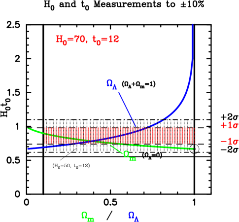
Figure 2: H₀t₀ versus $\Omega$ for H₀ = 70 km/sec/Mpc, t₀ = 12 Gyr, and uncertainties of $\pm$10% adopted for both ages. The dark line indicates the case of a flat Universe with $\rm\Omega_{\Lambda}+\Omega_{m}$ = 1. The abscissa in this case corresponds to $\rm\Omega_{\Lambda}$. The lighter curve represents a Universe with $\rm\Omega_{\Lambda}$ = 0. In this case, the abcissa should be read as $\rm\Omega_{m}$. The dashed and dot-dashed lines indicate 1-$\sigma$ and 2-$\sigma$ limits, respectively for values of H₀ = 70 km/sec/Mpc and t₀ = 12 Gyr in the case where both quantities are known to $\pm$10% (1-$\sigma$). The large open circle denotes values of H₀t₀ = 2/3 and $\Omega_{m}$ = 1 (i.e., those predicted by the Einstein-de Sitter model). Also shown for comparison is a solid line for the case H₀ = 50 km/sec/Mpc, t₀ = 12 Gyr.

9 Other Methods for Measuring H₀

Ultimately, for a value of H₀ and its uncertainty to be unambiguously established, it is essential to have several techniques that are based on completely different physics and assumptions. There are several methods for determining H₀ that are independent of the classical, extragalactic distance scale. These other methods offer a number of advantages. For example, the 3 methods described below, based respectively on the Sunyaev Zel’dovich effect, time delays of gravitational lenses, and cosmic microwave background anisotropies, all can be applied directly at very large distances, completely independent of the local extragalactic distance scale. However, to date, the numbers of objects, or measurements for these other techniques is still small, and the internal systematics have not yet been tested to the same extent as for the extragalactic distance scale. Recently, there has been progress in all of these areas, and ongoing and future experiments are likely to lead to rapid progress.

9.1 Distances Based on the Sunyaev Zel’dovich Effect

The underlying principle for this technique is similar to that described for other distance indicators in general: that is, the measurement of one distance–dependent, and one distance–independent quantity. An excellent recent review of this subject has been given by Birkinshaw birk99 .

As first described by Zel’dovich and Sunyaev sz69 , some of the low-energy cosmic microwave background (CMB) photons from the surface of last scattering scatter off of the hot electrons in the X-ray gas in clusters and generally gain energy through inverse Compton scattering. As a result, measurements of the microwave background spectrum toward rich clusters of galaxies show a decrement at lower frequencies (and a corresponding increase at higher frequencies). The size of the decrement thus depends on the density of electrons in the cluster and the path length through the cluster, but is completely independent of the cluster distance. The observed X-ray flux from the cluster is, however, dependent on the distance to the cluster. If it can be assumed that the cluster is spherically symmetric, the distance to the cluster can be solved for.

The greatest advantages of this method are that it can be applied directly at large distances and that it has an underlying physical basis. However, there are a number of astrophysical complications in the practical application of this method. For example, the gas distribution in clusters is not entirely uniform: that is, there is clumping of the gas (which, if present, would result in reducing $\rm H_{0}$), there are projection effects (if the clusters observed are prolate and seen end on, the true $\rm H_{0}$ could be larger than inferred). Furthermore, this method assumes hydrostatic equilibrium, and a model for the gas and electron densities, and, in addition, it is vital to eliminate potential contamination from other sources. The systematic errors incurred from all of these effects are difficult to quantify.

To date, a range of values of $\rm H_{0}$ have been published based on this method ranging from $\sim$40 - 80 km/sec/Mpc birk99 . Two-dimensional interferometry maps of the decrement are now becoming available; the most recent data for well-observed clusters yields H₀ = 60 $\pm$ 10 km/sec/Mpc. The systematic uncertainties are still large, but as more and more clusters are observed, higher-resolution X-ray maps and spectra, and Sunyaev–Zel’dovich maps, become available, the prospects for this method are improving enormously birk99 ; carlstrom . The accuracy of this method will be considerably improved when a sample of clusters has been identified independent of X-ray flux.

In Figure 3, a Hubble diagram of log d (distance) versus log z (redshift) is shown. Included in this plot are 4 clusters (Abell 478, 2142, 2256) with cz $<$ 30,000 (z$<$0.1) km/sec listed by Birkinshaw birk99 (his Table 7) as being clusters with reliable SZ measurements. These data are overplotted with the Key Project Cepheid and the secondary–method distances shown in Figure 1. These 4 clusters extend over the same current range as type Ia supernovae. Although SZ measurements are available out to significantly greater redshifts, beyond a redshift of $\sim$0.1, the effects of $\Omega_{m}$ begin to become significant. No SZ clusters at z$>$0.1 are shown. It is encouraging to see how consistent the results are over 2.5 decades in redshift. The local Cepheids (corrected for the local flow field) show more scatter, as expected. But a value of H₀ = 71 km/sec/Mpc is consistent with all of the data shown, from the local Cepheids out to type Ia supernovae and the Sunyaev–Zel’dovich clusters.

Figure 3: Top panel: A local plus far-field Hubble diagram of distance versus velocity including Cepheids, secondary distance indicators, plus Sunyaev Zel’dovich lens measurements extending to $\sim$30,000 km/sec. The nearby galaxy velocities have been corrected for the local flow field following Mould et al. mould99 . The symbols are as follows: Type Ia supernovae – squares, Sunyaev Zel’dovich method – solid circles with their published error bars – Tully–Fisher – solid circles, fundamental plane – solid triangles, surface brightness fluctuations – solid diamonds, Cepheids – open circles. A slope of H₀ = 71 is illustrated by the solid line. Dashed lines indicate $\pm$10%. The scatter in the far-field measurements is still significantly larger than for type Ia supernovae, but the results are consistent to within the current uncertainties. The prospects for decreasing the scatter in the Sunyaev Zel’dovich method appear very good in the near term as higher resolution interferometry and X-ray maps, for larger numbers of clusters become available.

9.2 Gravitational Lenses

A second method for measuring H₀ at very large distances, independent of the need for any local calibration, comes from the measurement of gravitational lenses. Refsdal ref64 ; ref66 showed that a measurement of the time delay and the angular separation for different images of a variable object such as a quasar can be used to provide a measurement of $\rm H_{0}$. This method offers tremendous potential not only because it can be applied at great distances, but it is based on very solid physical principles blandnar .

Difficulties with this method stem from the fact that astronomical lenses are extended galaxies whose underlying (luminous or dark) mass distributions are not independently known. Furthermore, they may be sitting in more complicated group or cluster potentials. A degeneracy exists between the mass distribution of the lens and the value of H₀ schech97 ; romankoch . Ideally velocity dispersion measurements as a function of position are needed to constrain the mass distribution of the lens. Such measurements are very difficult, but are recently becoming available tonryfranx . H₀ values based on this technique appear to be converging to about 60 km/sec/Mpc, although a range of 40 to 80 has been published schech97 ; romankoch ; tonryfranx ; impey98 .

9.3 Cosmic Microwave Background Anisotropies

The underlying physics governing the shape of the cosmic microwave background (CMB) anisotropy spectrum can be described by the interaction of a very tightly coupled fluid composed of electrons and photons before recombination huwhite ; sz70 . If the underlying source of the fluctuations is known, the power spectrum of fluctuations can be computed and compared with observations. Over the next few years, increasingly more accurate measurements will be made of the fluctuations in the CMB, offering the potential to measure a number of cosmological parameters. This field is becoming increasingly data rich with a number of planned and ongoing long-duration balloon experiments, and planned satellite experiments (e.g., MAP and Planck). Using the CMB data in combination with other data, for example, the Sloan survey, appears to be a promising way to break existing model degeneracies eisen , and measure a value for H₀.

10 The Future

A critical issue affecting the local determinations of H₀ remains the zero-point calibration of the extragalactic distance scale (more specifically, the Cepheid zero point). The most promising way to resolve this outstanding uncertainty is through accurate geometric parallax measurements. New satellite interferometers are currently being planned by NASA (the Space Interferometry Mission – SIM) and the European Space Agency (a mission known as GAIA) for the end of the next decade. These interferometers will be capable of delivering 2–3 orders of magnitude more accurate parallaxes than Hipparcos (i.e., a few microarcsec astrometry), reaching $\sim$1000$\times$ fainter limits. Accurate parallaxes for large numbers of Cepheids and RR Lyrae variables will be obtained. Moreover, in addition to improving the calibration for the distance to the LMC, it will be possible to measure rotational parallaxes for several nearby spiral galaxies, with distances accurate to a few percent.

Improvement to the photometric calibration for the HST Cepheid measurements will be possible with the Advanced Camera for Surveys (ACS), currently scheduled to fly in the year 2000. Next to the uncertainty in the distance to the Large Magellanic Cloud, the photometric zero point contributes the second largest source of systematic error in the determination of H₀. New ACS observations should quickly yield a higher accuracy than is currently possible with the Wide Field and Plantary Camera 2 now in use.

11 Concluding Remarks

Recent results on the determination of H₀ are encouraging. A large number of independent secondary methods (including the most recent type Ia supernova calibration by Sandage and collaborators saha99 ) appear to be converging on a value of H₀ in the range of 60 to 80 km/sec/Mpc. While only a few years ago, some published Cepheid distances to galaxies fmvict93 and values of H₀ differed by a factor of two , the $rms$ differences are now at a level of 10%. Given the historical difficulties in this subject, this is welcome progress. However, the need to improve the accuracy in the determination of H₀ is certainly not over. For an $rms$ uncertainty of 10%, the 95% confidence range restricts the value of H₀ only to 57 $<$ H₀ $<$ 85 km/sec/Mpc, underscoring the importance of reducing remaining errors in the distance scale (e.g., zero point, metallicity).

Even though there has been considerable progress recently, the current accuracy in H₀ is insufficient to discriminate between cosmological models that are open and those that are flat with non-zero $\Lambda$. Before compelling constraints can be made on cosmological models, it is imperative to rule out remaining sources of systematic error. With a value of H₀ accurate to 10% (1-$\sigma$) now available, it brings into sharper focus smaller (10-15%) effects which used to be buried in the noise in the era of factor-of-two discrepancies.

ACKNOWLEDGMENTS   It is a pleasure to contribute to this volume commemorating David Schramm. David was extremely encouraging to me, always rightfully skeptical, but very interested in the most recent observational results. I sincerely thank all of my collaborators on the extragalactic distance scale over the past 15 years, particularly B. F. Madore. In addition my thanks to all of the members of the HST H₀ Key Project team, whose enormous contributions enabled the Key Project to be undertaken: R. Kennicutt, J.R. Mould (co-PI’s), F. Bresolin, L. Ferrarese, H. Ford, B. Gibson, J. Graham, M. Han, P. Harding, J. Hoessel, J. Huchra, S. Hughes, G. Illingworth, D. Kelson, L. Macri, B.F. Madore, R. Phelps, A. Saha, S. Sakai, K. Sebo, N. Silbermann, P. Stetson, and A. Turner. Some of the results presented in this paper are based on observations with the NASA/ESA Hubble Space Telescope, obtained by the Space Telescope Science Institute, which is operated by AURA, Inc. under NASA contract No. 5-26555. Support for this work was provided by NASA through grant GO-2227-87A from STScI. This work has benefited from the use of the NASA/IPAC Extragalactic Database (NED).

References

- (1) E. W. Kolb & M. S. Turner The Early Universe, Addison-Wesley, New York, 1990.
- (2) J. A. Peacock Cosmological Physics, Cambridge University Press, Cambridge, 1999.
- (3) G. H. Jacoby, et al. Publ .Astron. Soc. Pac. 104 (1992) 599.
- (4) W. L. Freedman in Critical Dialogs in Cosmology, World Scientific, 1996, p. 92.
- (5) B. F. Madore & W. L. Freedman Publ. Astr. Soc. Pac. 103 (1991) 933.
- (6) W. L. Freedman & B. F. Madore in Clusters, Lensing and the Future of the Universe, ASP Conf. Series, eds. V. Trimble & Reisenegger, 1996.
- (7) R. Giovanelli, M. P. Haynes, J. J. Salzer, G. Wegner, L. N. Da Costa, & W. Freudling Astron. J. 116 (1998) 2632.
- (8) J. P. Cox, in Cepheids: Theory and Observations, ed. B. F. Madore, Cambridge University Press, 1985, pp. 126–146.
- (9) M. Livio, Type Ia Supernovae: Theory and Cosmology, Cambridge University Press, in press, 1999.
- (10) G. A. Tammann & A. R. Sandage Astrophys. J. 452 (1995) 16.
- (11) Hamuy, M., Phillips, M.M., Suntzeff, N.B. & Schommer, R.A. Astron. J 112 (1996) 2398.
- (12) Riess, A.G., Press, W.H. & Kirshner, R.P., Astrophys. J., 473 (1996) 88.
- (13) M. Phillips, Astrophys. J. Lett. 413 (1993) 105.
- (14) R. B. Tully & J. R. Fisher Astron. Astrophys. 54 (1977) 661.
- (15) M. Aaronson, G. Bothun, J. Mould, J. Huchra, R. A. Schommer, & M. E. Cornell Astrophys. J. 302 (1986) 536.
- (16) M. J. Pierce & R. B. Tully Astrophys. J. 330 (1988) 579.
- (17) R. Giovanelli, M. P. Haynes, N. P. Vogt, G. Wegner, J. J. Salzer, L. N. Da Costa, & W. Freudling Astron. J. 113 (1997) 22.
- (18) S. M. Faber & R. E. Jackson Astrophys. J. 204 (1976) 668.
- (19) A. Dressler, D. Lynden-Bell, D. Burstein, R. L. Davies, S. M. Faber, R. Terlevich & G. Wegner Astrophys. J. 313 (1987) 37.
- (20) G. Djorgovski & M. Davis, Astrophys. J. 313 (1987) 59.
- (21) I. Jorgensen, M. Franx & P. Kjaergaard Mon. Not. Roy. Astr. Soc. 280 (1996) 167.
- (22) J. Tonry & D. Schneider Astron. J. 96 (1988) 807.
- (23) J. Tonry in The Extragalactic Distance Scale,, eds., M. Livio, M. Donahue, & N. Panagia, Cambridge University Press, 1997, p. 297.
- (24) T. R. Lauer, J. L. Tonry, M. Postman, E. A. Ajhar, J. A. Holtzman Astrophys. J. 499 (1998) 577.
- (25) W. L. Freedman Ap. J. 326 (1988) 691.
- (26) W. L. Freedman & B. F. Madore Astrophys. J. 365 (1990) 186.
- (27) D. Sasselov et al. Astron. Astrophys. 324 (1997) 471.
- (28) C. S. Kochanek Astrophys. J. 491 (1997) 13.
- (29) R. C. Kennicutt et al. Astrophys. J. 498 (1998) 181.
- (30) W. L. Freedman Ap. J. 355 (1990) 35.
- (31) J. L. Tonry Astrophys. J. 373 (1991) 1.
- (32) R. C. Kennicutt, W. L., Freedman, & J. R. Mould, Astron. J. 110 (1995) 1476.
- (33) W. L. Freedman, B. F. Madore, J. R. Mould & R. C. Kennicutt in Cosmological Parameters and the Evolution of the Universe ed. K. Sato, Dordrecht, 1999, p. 17.
- (34) A. Sandage, A. Saha, G. A. Tammann, L. Lukas, N. Panagia, F. D. Macchetto Astrophys. J. 460 (1996) 15.
- (35) Tanvir, N.R., Shanks, T., Ferguson, H.C. & Robinson, D.R.T. Nature 377 (1995) 27.
- (36) Gibson, B.K., et al. 1999, Astrophys. J , submitted
- (37) Ferrarese, L., et al. 1999, Astrophys. J , submitted
- (38) Kelson, D.D., et al. 1999, Astrophys. J , submitted
- (39) Sakai, S., et al. 1999a, Astrophys. J , submitted
- (40) G. Jacoby, in The Extragalactic Distance Scale,, eds., M. Livio, M. Donahue, & N. Panagia, Cambridge University Press, 1997.
- (41) Mould, J.R., et al. 1999, Astrophys. J , submitted
- (42) W. Freedman et al. 2000, in preparation.
- (43) W. Freedman, (2000) in Particle Physics and the Universe, Nobel Symposium, World Scientific Publishing, in press.
- (44) B. E. Westerlund, in The Magellanic Clouds, (Cambridge: Cambridge Univ. Press, (1997).
- (45) W. L. Freedman & B. F. Madore in New Perspectives on Stellar Pulsation and Pulsating Variable Stars, eds. J.M. Nemec & J.M. Matthews, Cambridge Univ. Press: Cambridge, 1993, p. 92.
- (46) S. van den Bergh, Astrophys.J. 446 (1995) 39.
- (47) A. R. Walker, Ap. J. Lett. 390 (1992) L81.
- (48) A. Saha, W. L. Freedman, J. G. Hoessel, & A. E. Mossman Astron. J. 104 (1992) 1072.
- (49) K. Z. Stanek, D. Zaritsky, & J. Harris Astrophys. J. 500 141.
- (50) J. R. Herrnstein, J. M. Moran, L. J. Greenhill, P. J. Diamond, M. Inoue, N. Nakai, M. Miyoshi, C. Henkel, A. Riess, Nature, in press, July 10, astro-ph/9907013.
- (51) E. Maoz, J. Newman, L. Ferrarese, M. Davis, W. L. Freedman, B. F. Madore, P. B. Stetson, S. Zepf, Nature, in prep.
- (52) A. Gould & O. Uza Astrophys. J. 494 (1998) 118.
- (53) N. Panagia, 1998 STScI preprint No. 1218.
- (54) A. Walker, in Post-Hipparcos Cosmic Candles, Kluwer Academic Publishers, the Netherlands, 1999, p. 125.
- (55) E. L, Turner, R. Cen & J. P. Ostriker Astron. J. 103 (1992) 1427.
- (56) X. Shi & M. S. Turner Astrophys. J. 493 (1997) 519.
- (57) Y. Wang, D. N. Spergel & E. L. Turner Astrophys. J. 498 (1998) 1.
- (58) A. Kogut et al. Astrophys. J. 419 (1993) 1.
- (59) D. J. Fixsen et al. Astrophys. J. 420 (1994) 455.
- (60) M. Turner, in 1990 Nobel Symposium: The Birth and Early Evolution of Our Universe, Dark Matter in the Universe, 1991.
- (61) P. Coles & G. F. R. Ellis Nature 370 (1994) 609.
- (62) N. A. Bahcall & X. Fan Proc. Natl. Acad. Sci 95 (1998) 5956.
- (63) A. Riess et al. Astron. J. 116 (1998) 1009.
- (64) S. Perlmutter et al. Astrophys. J. 517 (1999) 565.
- (65) D. N. Schramm, in Astrophysical Ages and Dating Methods, eds. E. Vangioni-Flam et al. (Edition Frontieres: Paris, 1989).
- (66) J. W. Truran in The Extragalactic Distance Scale,, eds., M. Livio, M. Donahue, & N. Panagia, Cambridge University Press, 1997, p. 18.
- (67) T. D. Oswalt, J. A. Smith, M. A. Wood & P. Hintzen, Nature, 382, 692.
- (68) J. Bergeron, M. T. Ruiz & S. K. Leggett Astrophys. J. Suppl. 108 (1997) 339.
- (69) A. Renzini, in Observational Tests of Inflation, ed. T. Shanks et al. (Dordrecht, Kluwer, 1991), pp. 131-146.
- (70) D. A. VandenBerg, M. Bolte, and P. B. Stetson, Ann. Rev. Astron. Astrophys. 34 (1996) 461.
- (71) B. Chaboyer, P. Demarque, P. J. Kernan and L. M. Krauss, science 271 (1996) 957.
- (72) P. Demarque in The Extragalactic Distance Scale,, eds., M. Livio, M. Donahue, & N. Panagia, Cambridge University Press, 1997, p. 30.
- (73) N. Reid, Astron. J. 114 (1997) 161.
- (74) B. Chaboyer, P. Demarque, P. J. Kernan & L. M. Krauss, Astrophys. J 494 (1998) 96.
- (75) F. Pont, M. Mayor, C. Turon & D. A. Vandenberg Astron. & Astrophys. 329 (1998) 87.
- (76) W. L. Freedman et al., Nature , 371 (1994) 757.
- (77) W. L. Freedman Eighteenth Texas Symposium on Relativistic Astrophysics and Cosmology, eds. A. V. Olinto, J. A. Frieman & D. N. Schramm, World Scientific, p. 188.
- (78) M. Birkinshaw Phys. Rep., 310 (1999) 97.
- (79) Y. B. Zel’dovich & R. A. Sunyaev Astrophy. Sp. Sci. 4 (1969) 301.
- (80) J. Carlstrom et al. Bull. Amer. Astron. Soc. 194 (1999) 5801.
- (81) S. Refsdal Mon. Not. Roy Astr. Soc. 128 (1964) 295.
- (82) S. Refsdal Mon. Not. Roy Astr. Soc. 132 (1966) 101.
- (83) R. Blandford and R. Narayan, Ann. Rev. Astr. Astrophys 30 (1992) 311.
- (84) P. Schechter et al. Astrophys. J. 475 (1997) 85.
- (85) A. J. Romanowsky & C. S. Kochanek Astrophys. J. 516 (1999) 18.
- (86) M. Franx & J. Tonry Astrophys. J. 515 (1999) 512.
- (87) C. D. Impey et al. Astrophys. J. 509 (1998) 551.
- (88) W. Hu & M. White Astrophys. J. 441 (1996) 30.
- (89) R. A. Sunyaev & Y. B. Zel’dovich, Astr. Space Sci. 7 (1970) 3.
- (90) D. J. Eisenstein, W. Hu & M. Tegmark Astrophys. J. 518 (1999) 2.
- (91) A. Saha, A. Sandage, G. A. Tammann, L. Labhardt, F. D. Macchetto, N. Panagia, Astrophys. J., 000 (1999) 000, in press.