Using Perturbative Least Action to Run N Body Simulations Back in Time

Abstract

In this report, we present a new method for reconstructing N body initial conditions from a proscribed final density field. This method, Perturbative Least Action (PLA) is similar to traditional least action approaches, except that orbits of particles are found as expansions around previously determined and physically motivated orbits.

1 Introduction

In order to understand the current dynamics and history of large scale structure, it would be helpful if we were able to generate plausible initial conditions which would produce structure consistent with observations. One of the great difficulties with this problem is that it is fundamentally ill-posed, since much of the structure of interest is highly nonlinear. Many different initial conditions can give rise to virtually indistinguishable final density fields, even if all of them obey the constraints given by the Zel’dovich approximation.

We present the idea that even highly nonlinear $N$ body simulations may be self-consistently run backwards in time. While previous attempts at this problem, such as those by Peebles (1989, 1994), Shaya et al. (1995,1999), and Giavalsco et al. (1993), have suggested using the least action variational principle to solve the orbits of many particles, this approach yields the unfortunate result that only one of the potential solutions (namely, the first infall solution) can be recovered. We suggest the novel approach that by using least action as a perturbation from a known set of (randomly generated) orbits, a unique solution may be found for that set of initial conditions. By performing this analysis with many randomly selected sets of initial conditions, many sets of self-consistent solutions may be found. In this way, we may generate realistic initial conditions for interesting observed structure.

2 Method

The least action variational principle states that given a initial and final positions, a set of particles acting under mutual gravitation will take the path which minimizes the action (Peebles 1989):

$$S\equiv\sum_{i}\int_{0}^{t_{0}}dt\frac{a^{2}\dot{\bf x}^{2}_{i}}{2}-\frac{\phi_{i}}{2}$$ (1)

where ${\bf x}_{i}$ is the position of the $i^{th}$ particle given in comoving coordinates, and $\phi_{i}$ is the potential on the $i^{th}$ particle produced by all the others.

However, let us say that we know that some path ${\bf x}_{i}^{(0)}(t)$ minimizes the action (e.g. the output from an $N$ body code). In that case, we may imagine another path:

$${\bf x}_{i}(t)={\bf x}_{i}^{(0)}(t)+{\bf x}_{i}^{(1)}(t)\ ,$$ (2)

where ${\bf x}_{i}^{(1)}(t_{i})$ gives the change in the initial density field. Since we know that the action is minimized for the original path, we may write down the action for this new path as:

$$S=S^{(0)}+\sum_{i}\int_{0}^{t_{0}}dt\left(a^{2}\dot{\bf x}_{i}^{(0)}\cdot\dot{\bf x}_{i}^{(1)}+\frac{a^{2}\dot{\bf x}^{(1)2}_{i}}{2}-\frac{\phi_{i}}{2}+\frac{\phi^{(0)}_{i}}{2}\right)$$ (3)

If we parameterize the perturbation of the paths as:

$${\bf x}^{(1)}_{i}(t)=D(t){\bf x}^{(1)}_{i}(t_{0})+\sum_{n}C_{in}^{\alpha}f_{n}(t)\ ,$$ (4)

where $D(t)$ is the growth factor of perturbations as given in linear theory, $\alpha=\{1,2,3\}$ is direction of the vector, and $f_{n}(t)$ are a set of basis functions, then the perturbed action (and hence the total action), can be minimized when

$$\frac{\partial S^{(1)}}{\partial C_{in}^{\alpha}}=\int dt\left[\dot{f}_{n}(t)a^{2}\dot{\bf x}^{(1)}+f_{n}\left(\frac{\partial\phi^{(0)}_{i}}{\partial x^{\alpha}}-\frac{\partial\phi_{i}}{\partial x^{\alpha}}\right)\right]=0\ .$$ (5)

Note that the derivative of the first term in equation (3) is equivalent to the middle term in equation (5) by virtue of the fact that ${\bf x}^{(0)}$ is required to minimize action.

Using these equations, a randomly generated particle field (e.g. a Gaussian random field from some given power spectrum) may be iterated toward some target density field in the following way.

First, a set of initial conditions are created using the Zel’dovich approximation and known power spectrum. Next, the particle positions and velocities are evolved and recorded using some Poisson solver. For our simulations, we have used a straight Particle Mesh (PM) code. We then compare the final particle field to the target density field. Next, we determine perturbations (values of ${\bf x}_{i}^{(1)}(t_{0})$) which would cause the final density field to more strongly match the target field. Using those perturbations, we find the values of $C_{in}^{\alpha}$ which solve equation( 5). Using those coefficients, we determine the change in positions (and hence density) of the particles at high redshift, which gives us a new set of initial conditions. This new set of initial conditions can be run through the $N$ body code, and the process may be iterated until a satisfactory fit is returned.

While the perturbed initial field is not, strictly speaking, Gaussian random, it does obey the Zel’dovich approximation by an appropriate selection of basis functions. Moreover, since the unperturbed initial field was Gaussian random, and since the perturbative least action approach aims to find the closest set of initial conditions to those randomly generated (as illustrated in Figure 1) which will satisfy the proscribed final conditions, the solution will be fairly close to Gaussian random and as close as possible to the given power spectrum.

3 Simulations

As a test of this scheme, we create a highly nonlinear target density field with three overlapping isothermal spheres, with peaks as high as $\delta=5$. We then take two different sets of initial density fields (realizations of the same power spectrum), and iterate using the Perturbative Least Action (PLA) principle. We use a Particle Mesh code as our Poisson solver.

The simulations are each $64^{3}$ gridcells and $32^{3}$ particles, and were run from $z=99$ to $z=0$. Twenty timeslices or positions and velocities are used in order to do the least action integration. Around six iterations (i.e. computation of the least action, and running the result through the PM code) were necessary to produce the results shown.

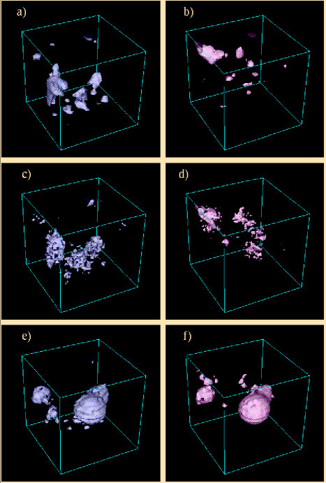
Figure 1: The results of a set of simulations. Panels a-b show two random realizations of the initial power spectrum. Panels c-d show the perturbed initial fields (after solving using least action). Panels e-f show the perturbed fields after having been run through the PM code.

Figure 1 shows the results of these simulations. The top row of panels show two randomly generated density fields at z=99. The velocity fields in each are given by the Zel’dovich approximation. By applying perturbative least action to each of these sets of initial fields with a particular target final density field, a new set of “perturbed” initial fields may be created.

The second row shows the perturbed initial fields. Notice that the large scale perturbations remain unchanged, and that only the small scale perturbations seem affected. This is due to the fact that we have specified the target field on a cell by cell basis, necessitating a very large amount of small scale power. Finally, the bottom panels show the result of integrating from our perturbed initial conditions. Despite the widely different initial conditions, both final fields strongly resemble both each other and the target field.

Though this toy problem is presented as proof of method, it is clear that this principle is applicable to a number of more complex problems such as determination of small scale primordial power, cluster redshift surveys, and study of the Local Group. This last would be quite interesting as recent studies (see e.g. Mateo 1998, and references therein) give a rather detailed picture of the current local density field and a series of simulations which could provide insight into probable infall scenarios would be most illuminating.

- [1] iavalisco, M., Mancinelli, B., Mancinelli, P. J., & Yahil, A. 1993, ApJ, 411, 9
- [2] ateo, M. 1998, ARA&A, 36, 435
- [3] eebles, P.J.E. 1989, ApJ, 344, L53
- [4] eebles, P.J.E. 1994, ApJ, 429, 43
- [5] haya, E.J., Peebles, P.J.E., & Tully, R.B. 1995, ApJS454, 15S
- [6] haya, E.J., Peebles, P.J.E., & Phelps, S.D. 1999, in this volume.