On the Evolution of Moving Groups: An Application to the Pleiades Moving Group

Abstract

The disruption of stellar systems, such as open clusters or stellar complexes, stands out as one of the most reasonable physical processes accounting for the young moving groups observed in the solar neighbourhood. In the present study we analyse some of the mechanisms that are important in the kinematic evolution of a group of unbound stars, such as the focusing phenomenon and its ability to recover the observed moving group’s velocity dispersions, and the efficiency of disc heating and galactic differential rotation in disrupting unbound stellar systems. Our main tools used to perform this analysis are both the epicycle theory and the integration of the equations of motion using a realistic gravitational potential of the Galaxy.

The study of the trajectories followed by stars in each of the Pleiades moving group substructures found by Asiain et al. Asiain et al. (1999) allows us to determine their stellar spatial and velocity distribution evolution. The kinematic properties of these substructures are compared to those of a simulated stellar complex which has evolved under the influence of the galactic gravitational potential and the disc heating. We conclude that a constant diffusion coefficient compatible with the observational heating law is able to explain the velocity and spatial dispersions of the Pleiades moving group substructures that are younger than $\sim 1.5\cdot 10^{8}$ yr.

1 Introduction

A “supercluster” can be defined as a group of stars gravitationally unbound that share the same kinematics and may occupy extended regions of the Galaxy. A “moving group” (MG hereafter) or “moving cluster”, however, is the part of the supercluster that can be observed from the Earth (see, for instance, Eggen 1994).

Independent of the physical process that leads to the formation of superclusters, there are basically two factors acting against their persistence in the general stellar background. First, when a group of unbound stars concentrated in the phase space has a certain velocity dispersion, the galactic differential rotation tends to spread them out very quickly in the direction of the galactic rotation (e.g., Woolley 1960). Second, observations show that the velocity dispersion of disc stars is increased with their age, which is usually interpreted as the result of a continuous process of gravitational acceleration that may be produced by different agents (e.g., Lacey 1991). This second factor, generally referred to as disc heating, also disperses stars very efficiently. It is therefore striking to verify that some of the classical MGs are several $10^{8}$ yr old. Some authors have overcome part of this problem by assuming that the velocity dispersion of these stellar groups must be very small – e.g. Eggen Eggen (1989), Yuan & Waxman Yuan & Waxman (1977), Soderblom & Mayor Sodermblom & Mayor (1993). Nevertheless, some recent studies Chen et al. (1997); Sabas (1997); Figueras et al. (1997); Chereul et al. (1998); Asiain et al. (1999) do not support such a small dispersions.

There have been several attempts to explain the origin of superclusters. Perhaps one of the most widely accepted explanation is the “evaporation” of the outermost stellar component (or corona) of open clusters (e.g. Efremov 1988). Over time, open clusters are disrupted by the gravitational interaction with massive objects in the Galaxy (such as giant molecular clouds), and as a result the open cluster members fill a long tube in space. The part of this tube that we can observe should have a small velocity dispersion – e.g. Weidemann et al. Weidemann et al. (1992), Eggen Eggen (1994). Although based in old stellar evolutionary models by Iben Iben (1967), Wielen Wielen (1971) found that about 50% of the open clusters disintegrate in less than 2$\cdot$10⁸ years, a result supported by posterior studies Terlevich (1987); Theuns (1992). If superclusters come from the evaporation of open clusters’s coronae, then Wielen’s Wielen (1971) results indicate that most superclusters should be young or the last tracers of former clusters.

MGs may also be produced by the dissolution of larger stellar agglomerations, such as stellar complexes or fragments of old spiral arms Woolley (1960); Wielen (1971); Yuan (1977); Elmegreen (1985); Efremov (1988); Comerón et al. (1997). Thus, a MG could be a mixture of stars coming from different open clusters’ coronae and disrupted associations that share the same origin (and motion). This process of MG formation includes the first hypothesis mentioned here. Alternatively, Casertano et al. Casertano et al. (1993) proposed that MGs are open clusters that evolved under the gravitational influence of a large local mass that surrounds and traps them. However, it seems difficult to specify the nature of such a large mass. Finally, it has been proposed that superclusters could actually be made of stars trapped around stable periodic orbits (e.g. Müllari et al. 1994; Raboud et al. 1998).

In this paper we assume that superclusters occupied a small volume in the phase space in their first stages, when they became gravitationally unbound. From that point on, they evolved under the influence of the gravitational potential of the Galaxy, as it would be the case in the classical picture of stellar evaporation from open clusters’ coronae. We then analyse different aspects related to the evolution of MGs.

First, in Sect. 2 we use epicycle approximation to study the ability of the “focusing phenomenon” Yuan (1977) to periodically group MG stars when no disc heating is considered. In Sect. 3 we show how to determine the stellar trajectories from an analytic expression of the galactic potential. The disc heating effect on moving groups’ properties can be considered by introducing random perturbations to the velocity components of stars. These trajectories allow us to study the evolution of unbound stellar systems independent of the local galactic properties (in contrast with epicycle approximation).

We focus our study on the origin and evolution of the Pleiades moving group, since it is the youngest moving group in the solar neighbourhood and, therefore, we may find it easier to recover its past properties with certain confidence (Sect. 4). We consider the different Pleiades substructures found in Asiain et al. (1999, Paper I), and estimate their kinematic age and galactic position at birth. Finally, in Sect. 5 we simulate a stellar complex and determine the trajectory of its stars to study its disruption over time. The disc heating effect on the evolution of the stellar complex is evaluated.

2 The focusing phenomenon

The epicycle approximation allows us to study, in an analytical way, the evolution of an unbound system of stars under the influence of the galactic potential. Under such approximation, the equations of motion of stars can be expressed as:

$$\xi^{\prime} = \xi^{\prime}_{a}+\xi^{\prime}_{b}\cos(\kappa t+\phi)$$

$$\eta^{\prime} = \eta^{\prime}_{a}-2\mbox{A}\xi^{\prime}_{a}t-\displaystyle\frac{2\omega_{\circ}\xi^{\prime}_{b}}{\kappa}\sin(\kappa t+\phi)$$

$$\zeta^{\prime} = \zeta^{\prime}_{a}\cos(\nu t+\psi)$$ (1)

in the coordinate system ($\xi^{\prime},\eta^{\prime},\zeta^{\prime}$) centered at the current position of the Sun. $\xi^{\prime}$ points towards the galactic center (GC), $\eta^{\prime}$ is a linear coordinate measured along a circumference of radius R_∘ (galactocentric distance of the Sun) and positive in the sense of the galactic rotation (GR), and $\zeta^{\prime}$ points towards the north galactic pole (NGP). $\kappa$ is the epicyclic frequency, $\nu$ is the vertical frequency, $t$ is the time (=0 at present) and $\omega_{\circ}$ is the angular velocity of the Galaxy at the current position of the Sun. $\xi^{\prime}_{a},\xi^{\prime}_{b},\eta^{\prime}_{a},\zeta^{\prime}_{a},\phi$ and $\psi$ are integration constants related to the current position and velocity of a star ($\xi^{\prime}_{\circ}$, $\eta^{\prime}_{\circ}$, $\zeta^{\prime}_{\circ}$, $\dot{\xi}^{\prime}_{\circ}$, $\dot{\eta}^{\prime}_{\circ}$, $\dot{\zeta}^{\prime}_{\circ}$) as:

$$\xi^{\prime}_{a} = -\displaystyle\frac{2\xi^{\prime}_{\circ}\omega_{\circ}+\dot{\eta}^{\prime}_{\circ}}{2\mbox{B}}\vspace{.15cm}$$

$$\xi^{\prime}_{b} = -\left[\left(\displaystyle\frac{2\mbox{A}\xi^{\prime}_{\circ}+\dot{\eta}^{\prime}_{\circ}}{2\mbox{B}}\right)^{2}+\left(\displaystyle\frac{\dot{\xi}^{\prime}_{\circ}}{\kappa}\right)^{2}\right]^{1/2}\vspace{.15cm}$$

$$\eta^{\prime}_{a} = \eta^{\prime}_{\circ}-\displaystyle\frac{2\omega_{\circ}\dot{\xi}^{\prime}_{\circ}}{\kappa^{2}}\vspace{.15cm}$$

$$\zeta^{\prime 2}_{a} = \zeta^{\prime 2}_{\circ}+\displaystyle\frac{\dot{\zeta}^{\prime 2}_{\circ}}{\nu^{2}}\vspace{.15cm}$$

$$\phi = \arctan\left(\displaystyle\frac{-2\dot{\xi}^{\prime}_{\circ}\mbox{B}}{\kappa(\dot{\eta}^{\prime}_{\circ}+2\xi^{\prime}_{\circ}\mbox{A})}\right)\vspace{.15cm}$$

$$\psi = \arctan\left(\displaystyle\frac{-\dot{\zeta}^{\prime}_{\circ}}{\nu\zeta^{\prime}_{\circ}}\right)\mbox{ ,}$$ (2)

where the B and A are the Oort’s constants. In A we use Eqs. 2 to evaluate the evolution of space and velocity dispersions of a group of stars with low peculiar velocity with respect to their Regional Standard of Rest (RSR). Eqs. A show that dispersions in position and velocity components oscillate around constant values, except for the azimuthal coordinate $\eta^{\prime}$, whose dispersion $\sigma_{\eta^{\prime}}$ increases with $t$. After a few $10^{7}$ yr, this increase is dominated by the secular terms for typical position and velocity dispersions of young stellar groups, and it can be approximated by the linear relationship

$$\sigma_{\eta^{\prime}}=\displaystyle\frac{\mbox{A}}{\mbox{B}}\left(4\omega_{\circ}^{2}\sigma_{\xi^{\prime}_{\circ}}^{2}+\sigma_{\dot{\eta}^{\prime}_{\circ}}^{2}\right)^{1/2}t\;\mbox{ . }$$ (3)

If we consider a sample of stars with $\sigma_{\xi^{\prime}_{\circ}}\approx$ 0 pc and $\sigma_{\dot{\eta}^{\prime}_{\circ}}\approx$ 0 km s^-1, then all dispersions in position and velocity would oscillate around their mean values with an epicycle frequency $\kappa$. Stars would meet every $\Delta t=\displaystyle\frac{2\pi}{\kappa}$ (at the position of the Sun $\Delta t\approx 1.5\cdot 10^{8}$ yr), a fact that has been referred to as “focusing phenomenon” Yuan (1977). However, when we apply Eq. 3 to a more realistic case where dispersions are close to those of the open clusters and associations, i.e. a few parsecs in $\sigma_{\xi^{\prime}_{\circ}}$ and $\sim$ 1-2 km s^-1 in $\sigma_{\dot{\eta}^{\prime}_{\circ}}$, we obtain $\sigma_{\eta^{\prime}}\approx$ 1 kpc after a $t\approx$ 5-10 $\cdot 10^{8}$ yr – a period of time shorter than the age of some moving groups detected in the solar neighbourhood (e.g. Chen et al. 1997; Paper I). Thus, galactic differential rotation disrupts very efficiently unbound systems of stars. Nonetheless, if the distribution of stars in $\eta^{\prime}$ is supposed to be gaussian after the disruption of the stellar system, an important proportion of the original sample will be still concentrated in space after a long period of time; for instance, for $\sigma_{\eta^{\prime}_{\circ}}$ = 1 kpc we can find still $\sim$ 24 % of the initial stars in a region 600 pc long in $\eta^{\prime}_{\circ}$ after 5-10 $\cdot 10^{8}$ yr.

3 Stellar trajectories

The epicycle approximation holds for stars that follow almost circular orbits around the center of the Galaxy. Although valid for most of our stars, some of them, with high peculiar velocities with respect to the Local Standard of Rest (LSR), perform radial galactic excursions of a few kpc in length. The galactic gravitational potential changes significatively at different points of their trajectories, and so the first order approximation is no longer valid. In addition, the vertical motion is poorly described by a harmonic oscillation as stars gain certain height over the galactic plane. For a more rigorous analysis, we need to use a realistic model of the galactic gravitational potential. Stellar orbits will be determined from this model by integrating the equations of motion (Sect. 3.1). Moreover, the addition of a constant scattering in this process will allow us to account for the disc heating effect on the stellar trajectories (3.2).

3.1 The galactic potential

Expressed in a cartesian coordinate system ($\xi,\eta,\zeta$) centered at the position of the Sun and rotating at a constant angular velocity $\omega_{\circ}$,

$$\omega_{\circ}=\sqrt{\displaystyle\frac{1}{R_{\circ}}\;\;\Biggl{(}\frac{\partial\Phi}{\partial R}\Biggr{)}_{\circ}}\;\;\mbox{ ,}$$ (4)

the equations of motion of a star, assuming that the gravitational potential of the Galaxy $\Phi_{\mathrm{G}}(R,\theta,z;t)$ (in cylindrical coordinates centered on the GC) is known, are:

$${\ddot{\xi}} = -\displaystyle\frac{\partial\Phi_{\mathrm{G}}}{\partial\xi}-\omega_{\circ}^{2}(R_{\circ}-\xi)-2\omega_{\circ}\dot{\eta}$$

$${\ddot{\eta}} = -\displaystyle\frac{\partial\Phi_{\mathrm{G}}}{\partial\eta}+\omega_{\circ}^{2}\eta+2\omega_{\circ}\dot{\xi}$$

$${\ddot{\zeta}} = -\displaystyle\frac{\partial\Phi_{\mathrm{G}}}{\partial\zeta}\;\;\mbox{ .}$$ (5)

A fourth order Runge-Kutta integrator allows us to numerically solve these equations when $\Phi_{\mathrm{G}}$ is known, obtaining the trajectory of the star. To get a realistic estimation of the galactic gravitational potential we decompose it into three parts: the general axisymmetric potential $\Phi_{\mathrm{AS}}$, the spiral arm $\Phi_{\mathrm{Sp}}$, and the central bar $\Phi_{\mathrm{B}}$ perturbations to the first contribution, i.e.

$$\Phi_{\mathrm{G}}=\Phi_{\mathrm{AS}}+\Phi_{\mathrm{Sp}}+\Phi_{\mathrm{B}}\mbox{ .}$$

We adopt the model developed by Allen & Santillán Allen & Santillán (1991) for the axisymmetric part of the potential, $\Phi_{\mathrm{AS}}(R,z)$, because of both its mathematical simplicity – which allows us to determine orbits with a very low CPU consumption – and its updated parameters. The model consists of a spherical central bulge and a disk, both of the Miyamoto-Nagai Miyamoto & Nagai (1975) form, plus a massive spherical halo. This model is symmetrical with respect to an axis and a plane. The authors adopted the recommendations of the IAU Kerr & Lynden-Bell (1986) for the galactocentric distance of the Sun ($R_{\circ}$ = 8.5 kpc) and the circular velocity at the position of the Sun ($\Theta_{\circ}$= 220 km s^-1). The Oort constants derived from this model are well within the currently accepted values.

Spiral arm perturbation to the potential is taken from Lin and associates’ theory (e.g. Lin 1971 and references therein), that is:

$$\Phi_{\mathrm{Sp}}(\mbox{R},\theta;t)={\cal A}\cos(m(\Omega_{p}t-\theta)+\phi(R))\;\;\mbox{ ,}$$ (6)

where

$${\cal A} = \displaystyle\frac{(R_{\circ}\omega_{\circ})^{2}f_{r0}\tan i}{m}\mbox{ ,}$$

$$\phi(R) = -\displaystyle\frac{m}{\tan i}\ln\left(\displaystyle\frac{R}{R_{\circ}}\right)+\phi_{0}\mbox{ .}$$

${\cal A}$ is the amplitude of the potential, $f_{r0}$ is the ratio between the radial component of the force due to the spiral arms and that due to the general galactic field. $\Omega_{p}$ is the constant angular velocity of the spiral pattern, $m$ is the number of arms, $i$ is the pitch angle, $\phi$ is the radial phase of the wave and $\phi_{0}$ is a constant that fixes the position of the minimum of the spiral potential. According to Yuan Yuan (1969), we adopt $f_{r0}=0.05$ (this value has been confirmed in a recent study by Fernández, 1998) and $\Omega_{p}=13.5$ km s^-1 kpc^-1.

We consider a classical two arm pattern ($m=2$) Yuan (1969); Vallée (1995). If we assume that the Sagittarius arm is located at a galactocentric distance R${}_{Sag}=$ 7.0 kpc, and that the interarm distance in the Sun position is $\Delta R=$3.5 kpc as suggested by observations on spiral arm tracers Becker & Fenkart (1970); Georgelin & Georgelin (1976); Liszt (1985); Kurtz et al. (1994), then the pitch angle can be determined to be:

$$\tan i=\displaystyle\frac{m}{2\pi}\ln(1+R_{Sag}^{-1}\;\Delta R)\mbox{ .}$$ (7)

For $m=2$, we obtain $i=7\aas@@fstack{\circ}35$ (close to the Yuan’s (1969) value $i=6\aas@@fstack{\circ}2$).

For $t=0$ and $\theta=0\degr$, the adopted value $\phi_{0}$ leads to a minimum in the potential at the observed position of the Sagittarius arm (R = R${}_{Sag}\leavevmode\nobreak\ =\leavevmode\nobreak\ 7.0$ kpc, $l=0\degr$). $\phi_{0}$ can thus be expressed as:

$$\phi_{0}=\pi+\displaystyle\frac{m}{\tan i}\ln\left(\displaystyle\frac{R_{Sag}}{R_{\circ}}\right).$$ (8)

For $i=7\aas@@fstack{\circ}35$ and $m=2$ we obtain $\phi_{0}=$ 0.131 rad.

The central bar potential we use here is, for simplicity, a triaxial ellipsoid with parameters taken from Palous̆ et al. Palous̆ et al. (1993), i.e.

$$\Phi_{b}(\mbox{R},\theta,z;t)=-\displaystyle\frac{GM_{bar}}{\left(q_{bar}^{2}+x^{2}+\displaystyle\frac{a_{bar}^{2}}{b_{bar}^{2}}y^{2}+\displaystyle\frac{a_{bar}^{2}}{c_{bar}^{2}}z^{2}\right)^{1/2}},$$ (9)

where $x=\mbox{R}_{\circ}\cos(\theta-\Omega_{B}t-\theta_{\circ})$ and $y=\mbox{R}_{\circ}\sin(\theta-\Omega_{B}t-\theta_{\circ})$, with $\theta_{\circ}=$ 45$\degr$ Whitelock & Catchpole (1992). $a_{bar},b_{bar}$ and $c_{bar}$ are the three semi-axes of the bar, with $q_{bar}$ its scale length, and with $\displaystyle\frac{a_{bar}}{b_{bar}}=\displaystyle\frac{1}{0.42}$, $\displaystyle\frac{a_{bar}}{c_{bar}}=\displaystyle\frac{1}{0.33}$, and $q_{bar}=5$ kpc. The adopted total mass of the bar, $M_{bar}$, is $10^{9}$ M_⊙, and its angular velocity, $\Omega_{B}$, is 70 km s^-1 kpc^-1 Binney et al. (1991). Although most of the parameters that define the bar are very uncertain, the effect of the bar on the stellar trajectories becomes important only after several galactic rotations, which requires a length of time greater than the age of the stars considered in our study.

3.2 Disc heating in the stellar trajectories

The observational increase in the total stellar velocity dispersion ($\sigma$) with time ($t$), or disc heating, can be approximated by an equation of the form:

$$\sigma(t)^{n}=\sigma_{\circ}^{n}+C_{v}t\mbox{ ,}$$ (10)

where $\sigma_{\circ}$ is the dispersion at birth and $C_{v}$ the “apparent diffusion coefficient” Wielen (1977). The constants $n$, $\sigma_{\circ}$ and $C_{v}$ give one important information on the physical mechanism responsible for the disc heating Lacey (1991); Fridman et al. (1994).

Our sample of B and A main sequence type stars, described in Paper I, allows us to determine an accurate and detailed disc heating law for the last $10^{9}$ yr, given the quality and uniformity of our ages and the size of this sample (2 061 stars). A standard nonlinear least-squares method (Levenberg-Marquardt method) has been applied to fit the heating coefficients to our data (Fig. 1). In this way we obtain $\sigma_{\circ}\approx 12$ km s^-1, $n\approx 5$ and $C_{v}\approx 0.01$ (km s^-1)ⁿyr^-1, similar to Lacey’s Lacey (1991) results for $n=5$, i.e. $\sigma_{\circ}=15$ km s^-1 and $C_{v}=0.01$ (km s^-1)⁵yr^-1. When we fix $n$ to 2, we obtain $\sigma_{\circ}\approx 15$ km s^-1and $C_{v}\approx 5.6\cdot 10^{-7}$ (km s^-1)²yr^-1, which is again in agreement with Lacey’s Lacey (1991) ($\sigma_{\circ}=15$ km s^-1 and $C_{v}=5\cdot 10^{-7}$ (km s^-1)²yr^-1) and Wielen’s Wielen (1977) ($\sigma_{\circ}=10$ km s^-1 and $C_{v}=6\cdot 10^{-7}$ (km s^-1)²yr^-1) fits with $n=2$.

Our accurate observational heating law (circles in Fig. 1) is far from being smooth. Two special features can be observed on this law: first, the velocity dispersion shows a steep increase during the first $\sim 4\cdot 10^{8}$ yr, probably due to the phase mixing of young stars. After this point, this increase becomes less pronounced. Second, an almost periodic oscillation seems to be superimposed over the “continuous” heating law. This oscillation (period $\approx 3\cdot 10^{8}$ yr) could be the signature of an episodic event (see for instance Binney & Lacey 1988, Sellwood 1999).

Figure 1: Fit of Equation 10 to our data (see text), using stars closer than 300 pc from the Sun, with 100 stars per bin. Solid line: $\sigma_{\circ}$, $C_{v}$ and $n$ are fitted; dashed line: $\sigma_{\circ}$ and $C_{v}$ are fitted, whereas $n$ is fixed to 2. The error bars on points include only statistical uncertainties, calculated as $\epsilon_{\sigma}=\sigma/\sqrt{2N}$, where $N$ is the number of stars per bin

Figure 2: Velocity dispersion vs. time, determined by integrating the equations of motion of a simulated sample when an isotropic diffusion is applied at each time-step. Dashed line: observational fit to disc heating with a fixed slope $n$=2

Since we do not know the details about the mechanisms that perturb the stellar orbits and cause the disc heating effect, we assume for simplicity that the accelerating processes acting on a given star can be approximated by a sequence of independent and random perturbations of short duration Wielen (1977). In order to evaluate the magnitude of these perturbations we generated a sample of 500 stars located around the position of the Sun at $t=0$, and uniformly distributed in a 100 pc/side cube. Initially, these stars are moving with the same velocity as the LSR, with an isotropic dispersion in velocity $\sigma_{\circ}$. During the process of orbit determination, the velocity of the star is instantaneously changed by $\Delta\@vec{v}$ every $\Delta$ yr. This $\Delta\@vec{v}$ is normally distributed around zero with a (constant) isotropic dispersion $\sigma_{h}$ in each component. The equations of motion are integrated using only the axisymmetric part of the galactic potential ($\Phi_{\mathrm{AS}}$). This allows us to introduce the heating effect only through the parameter $\sigma_{h}$, avoiding possible redundances, such as the scattering of disc stars by spiral arms. The best approximation to the observational heating law is obtained when $\sigma_{h}=1.45$ km s^-1 for $\Delta t=10^{7}$ yr, and $\sigma_{\circ}\approx$ 15 km s^-1. It can be demonstrated that $\sigma_{h}$ and $\Delta t$ are related with the “true diffusion coefficient” $D$ introduced by Wielen Wielen (1977) just as $D=\displaystyle\frac{\sigma_{h}^{2}}{\Delta t}$. On the other hand $C_{v}=2.95\;D$, as demonstrated by Wielen Wielen (1977) using the epicycle theory. We obtain in this way an independent estimation of $C_{v}$, i.e. $C_{v}=2.95\;\displaystyle\frac{1.45^{2}}{10^{7}}=6.2\cdot 10^{-7}$ (km s^-1)²yr^-1. This value is in an excellent agreement with our previous estimation. In Figure 2 the evolution of the total velocity dispersion for this simulated sample is compared with the fit of Eq. 10 to the observational data when $n=2$, showing an excellent match. This procedure will be used in Sect. 5 to simulate the evolution of a stellar system under the influence of the disc heating.

4 The Pleiades Moving Groups

In Paper I we used a method based on non-parametric density estimators to detect MGs among a sample of 2 061 B and A main sequence type stars in the four-dimensional space (U,V,W,log (age) ). We used HIPPARCOS data as well as radial velocities from several sources (see Paper I for the details) to determine the stellar spatial velocities, and Strömgren photometry for the stellar ages. Tables 1 and 2 in Paper I show the main properties of the MGs when separated in the (U,V,W,log (age)) and (U,V,log (age)) spaces respectively. Since the W-velocity component is less discriminant than the other three variables, we will focus our study on the MGs in Table 2 of Paper I (Table 1 here). In particular, as already mentioned in the Sect. 1, we will deal with those MGS whose velocity components resemble those of Pleiades open cluster.

Table 1: Number of members ($\cal N$), velocity components and ages (along with their dispersions) of the Pleiades MGs found in Paper I

Moving	$\cal N$	U	V	W	$\tau$
Group		[km s-1]	[km s-1]	[km s-1]	[108 yr]
B1	34	-4.5(4.7)	-20.1(3.3)	-5.5(1.9)	0.2(0.1)
B2	75	-10.7(5.3)	-18.8(3.7)	-5.6(2.2)	0.6(0.2)
B3	50	-16.8(5.1)	-21.7(2.7)	-5.6(4.6)	3.0(1.2)
B4	53	-8.7(4.8)	-26.4(3.3)	-8.5(4.7)	1.5(0.5)

It is interesting to compare these results with those recently obtained by Chereul et al. Chereul et al. (1998), who also found similar substructures in the Pleiades and other MGs by means of a wavelet analysis performed at different scales. The velocity dispersions of their substructures are quite a bit larger than those found for classical MGs, in agreement with our results. In their analysis, they did not consider the stellar age as a discriminant variable, which prevents them from detecting those substructures that are strongly defined in age but not so well defined in the velocity components. Another important difference between both methods is that Chereul et al. Chereul et al. (1998) did not determine photometric ages for A0 to A3 stars, since no reliable metallicity is available for them. Instead, they computed a “paliative” age that produces an artificial peak in age of $10^{7}$ yr, and a lack of other young stars (up to $\sim 5\cdot 10^{8}$ yr). As mentioned in Asiain et al. Asiain et al. (1997), a metallicity $Z=0.02$ is representative, in a statistical sense, of (normal) A type stars. Using this value, we did not observe any lack of stars in the young part of the age distribution (Paper I). On the other hand, since we do not use F type stars in our study because of the high uncertainties involved in the process to determine their ages, our data do not allow us to confirm the existence of the $\sim 10^{9}$ yr old Pleiades substructure found by Chereul et al. Chereul et al. (1998).

Using the numerical integration procedure described in Sect. 3.1, and the mean properties (nuclei) of the Pleiades substructures found in Paper I (Table 1), we have computed the trajectories of these substructures from the present up to the moment they were born (Fig. 3). This latter age is defined as the average age of the MGs constituent members. The youngest group, i.e. B1, is composed of Scorpio-Centaurus (Sco-Cen) OB association members (Paper I), and it was born in the interarm region. In Sect. 4.1 we study the evolution of this group. Since B1 is still too young to be affected by the disc heating effect or phase space mixing, we can determine its kinematic age with some confidence. The B2 group is considered separately in Sect. 4.2. This is also quite a young group and contains accurate information on some of the closest associations. The birthplace of the older groups, i.e. B3 and B4, is close to a minimum of the spiral arm potential, which seems consistent with their being born around this structure. Details on their spatial and velocity evolution are given in Section 4.3.

In recent studies based on the velocity field of Cepheids, Mishurov et al. Mishurov et al. (1997) and Mishurov & Zenina Mishurov & Zenina (1999) obtained a set of spiral arm parameters which clearly differ from those adopted here (e.g., in Mishurov & Zenina Mishurov & Zenina (1999), $\phi_{0}=142\degr$ and $\Omega_{p}-\omega_{\circ}\approx 0.5$ km s^-1 kpc^-1). When considering these new parameters, all Pleiades MG substructures turn out to be also placed, at birth, around the spiral arms. In this particular case, the Pleiades substructures appear, at birth, concentrated in a small area of the Galaxy. We also tested that the main conclusions of the current paper does not critically change with the selection of any of this two spiral arm patterns, as expected.

Figure 3: Trajectories of the MG’s nuclei in Table 1 backwards in time, from present ($t=0$) until their mean age. The dashed lines represent spiral arms, as defined in Sect. 3.1. The reference system is rotating with the same angular velocity as the spiral arms ($\Omega_{p}$)

4.1 Scorpio-Centaurus association

Because of the short age of these stars and the quality of our data we are able to determine quite precisely these stars’ kinematic age, defined as the time at which they were most concentrated in space – assuming that they are gravitationally unbound. We consider here only those stars in B1 that are concentrated in space (see Fig.7 in Paper I). With the exception of HIP84970 and HIP74449, all of these stars were classified as members of Sco-Cen association by de Zeeuw et al. de Zeeuw et al. (1999) . Their position in the galactic and meridional planes as a function of time are shown in Figure 4. It is quite evident that between around 4 and 12 Myr ago these stars were closer to each other than they are at present. However, observational errors produce additional dispersions on velocity and position, and therefore the maximum spatial concentration we find is shifted to the present. Figure  4 also shows us that the last intersection of the Sco-Cen association with the galactic plane was between 8 and 16 million years ago.

Figure 4: Spatial distribution of the 27 stars in B1 sub-group that are spatially concentrated in space as a function of time. Numbers in the upper right corners indicate the time in Myr

The evolution of the errors or dispersions in the stellar position and velocity can be calculated more precisely by means of the epicycle approximation (Eqs. A). We now consider the fact that the observed dispersion in position inside a given MG ($\sigma_{{\rho},{\mathrm{o}bs}}$, where $\rho$ is the distance from the LSR to a given star) can be decomposed into two parts, i.e.

$$\sigma^{2}_{{\rho},{\mathrm{o}bs}}(t)=\sigma^{2}_{{\rho},{\mathrm{i}nt}}(t)+\sigma^{2}_{{\rho},{\mathrm{e}rr}}(t)\mbox{ ,}$$ (11)

where

$\sigma_{{\rho},{\mathrm{i}nt}}(t)$ is the MG intrinsic dispersion at the time $t$, and
$\sigma_{{\rho},{\mathrm{e}rr}}(t)$ is the MG mean observational error.

Since both $\sigma_{{\rho},{\mathrm{o}bs}}$ and $\sigma_{{\rho},{\mathrm{e}rr}}$ can be easily determined at different epochs ($\sigma_{{\rho},{\mathrm{o}bs}}(t)$ can be calculated by integrating the stellar orbits until time $t$, and $\sigma_{{\rho},{\mathrm{e}rr}}(t)$ can be propagated from present using Eqs. A), we can also derive the time $t_{\mathrm{m}in}$ at which $\sigma_{{\rho},{\mathrm{i}nt}}(t)$ was minimum. In Figure 5 we show the evolution of $\sigma_{{\rho},{\mathrm{o}bs}}$, $\sigma_{{\rho},{\mathrm{e}rr}}$ and $\sigma_{{\rho},{\mathrm{i}nt}}$. We observe a clear minimum in $\sigma_{{\rho},{\mathrm{i}nt}}$ around $t_{\mathrm{m}in}\approx 9\cdot 10^{6}$ yr, which corresponds to B1 kinematic age. At the minimum spatial concentration we find the intrinsic spatial dispersions are $\sigma_{\xi^{\prime}}$ = 20 pc, $\sigma_{\eta^{\prime}}$ = 22 pc, and $\sigma_{\zeta^{\prime}}$ = 15 pc, smaller than their current values of $\sigma_{\xi^{\prime}}$ = 30 pc, $\sigma_{\eta^{\prime}}$ = 33 pc, and $\sigma_{\zeta^{\prime}}$ = 16 pc. Also, their intrinsic velocity dispersions were smaller at $t_{\mathrm{m}in}$, and $\la$ 2 km s^-1 in each component.

Figure 5: Evolution of the observed dispersion (dot-dashed line), mean propagated error (dashed line) and intrinsic dispersion (solid darker line) in $\rho$ (distance to the Sun), determined from the most spatially concentrated stars in the B1 group

There is a clear discrepancy between the kinematic and the “photometric” age of B1. This could be due to several reasons. First of all, most of the stars in B1 are massive, and their atmospheres are probably rotating very quickly. Thus, the observed photometric colors are affected by this rotation, and so are the derived atmospheric parameters. The photometric ages, determined from these atmospheric parameters and stellar evolutionary models Asiain et al. (1997), are systematically overestimated because of this effect. In order to evaluate this effect, we have corrected the observed photometric colors for rotation by considering a constant angle of inclination between the line of sight and the rotation angle ($i=60^{\circ}$), and a constant atmospheric angular velocity ($\omega=0.6\;\omega_{c}$, where $\omega_{c}$ is the critical angular velocity). In this way we obtain a mean age $\approx 1.1\cdot 10^{7}$ yr, and even smaller values for $\omega>0.6\;\omega_{c}$. More details on the correction for atmospheric rotation can be found in Figueras & Blasi Blasi (1998). Second, before applying our method to detect moving groups (Paper I) we eliminated all stars with relative errors in age bigger than 100 %, which slightly bias the age of young groups to larger values.

In a recent study de Zeeuw et al. de Zeeuw et al. (1999) carried out a census of nearby OB associations using HIPPARCOS astrometric measurements and a procedure that combines both a convergent point method and a method that uses parallaxes in addition to positions and proper motions. Their sample of neighbouring stars is much larger than ours, since radial velocities and Strömgren photometry are needed for our analysis. They found 521 stars in the Sco-Cen association, of which only 65 were in our sample. From these stars we have determined the mean velocity components of each association, which are in close agreement to those of B1 (Table 2). However, their dispersions and ages are quite a bit larger than expected for a typical association. A deeper analysis revealed to us the presence of some stars in de Zeeuw et al.’s de Zeeuw et al. (1999) associations whose peculiar velocities are responsible for their large velocity dispersion. Consistently, the ages of these stars are also peculiar ($\tau\approx 1-5\cdot 10^{8}$ yr). Removing these stars and a few others with anomalously large ages, all of which probably belong to the field, we find a more reasonable kinematic properties and ages for these associations (Table 3).

Table 2: Number of members ($\cal N$), spatial velocity components and ages (along with their dispersions) of the Sco-Cen associations found by de Zeeuw et al. de Zeeuw et al. (1999), determined from those members present in our sample

Assoc.	$\cal N$	U	V	W	$\tau$
		[km s-1]	[km s-1]	[km s-1]	[108 yr]
US	14	-3.5(4.3)	-15.7(2.1)	-6.4(1.8)	0.4(0.5)
UCL	32	-3.7(7.0)	-19.7(4.1)	-4.9(2.1)	0.7(1.0)
LCC	19	-6.8(4.7)	-18.5(6.5)	-6.4(1.7)	0.9(1.2)
TOTAL	65	-4.6(6.1)	-18.5(4.9)	-5.7(2.1)	0.7(1.0)

Table 3: Same as Table 2, now removing a few stars with peculiar velocity components and ages

Assoc.	$\cal N$	U	V	W	$\tau$
		[km s-1]	[km s-1]	[km s-1]	[108 yr]
US	12	-3.8(4.0)	-15.5(2.1)	-6.6(1.8)	0.2(0.1)
UCL	28	-1.7(4.4)	-20.4(3.6)	-4.4(1.5)	0.4(0.3)
LCC	16	-5.1(2.7)	-20.6(4.0)	-6.0(1.6)	0.4(0.3)
TOTAL	56	-3.1(4.2)	-19.4(4.0)	-5.3(1.9)	0.4(0.3)

4.2 B2 group

Even though B2 is quite a young group, the propagation of age uncertainties over time prevents us from determining the group’s kinematic age by means of the procedure developed for the B1 group. Instead, we have determined the trajectories of each star in B2, and that of the MG’s nucleus itself. The spatial concentration of these stars is propagated back in time by counting the number of stars found in 300 pc around the MG nucleus (Fig. 6). We do not find any maximum in spatial concentration during the last $10^{8}$ yr. To better understand the structure of this group we plot in Fig. 7 the position of these stars and their velocity components on the galactic and meridional plane, referred to the LSR and corrected for galactic differential rotation. We observe that it is actually composed of several spatial stellar clumps, each of which has its own kinematic behaviour, although certain degree of mixture is also evident. In particular, one of these clumps (most of the filled circles in Fig. 7) perfectly overlaps with the Sco-Cen association mentioned above (20 of these stars are classified as members of this association by de Zeeuw et al. 1999). This clumps’s velocity components, and kinematic age, are also very similar to those found for the B1 group. Once again, the photometric age of these stars is probably overestimated because of the high rotation velocity of their atmospheres. A second clump is coincident with the Cassiopeia-Taurus (Cas-Tau) association in both position and velocity spaces (most of the empty circles in Fig. 7). There are two dominant streams among these stars. In the heliocentric system, corrected for galactic differential rotation, their velocities are (U,V)$\simeq$(-10,-18) km s^-1 and (-13,-23) km s^-1 respectively (they share a common W component $\sim-6$ km s^-1). Their ages are $5-6\cdot 10^{7}$ yr. These values are in good agreement with those found by de Zeeuw et al. de Zeeuw et al. (1999) for Cas-Tau association, i.e. (U,V,W) = (-13.24,-19.69,-6.38) km s^-1 with an age of $5\cdot 10^{7}$ yr (actually, about half of them are classified as Cas-Tau members by these authors). Finally, we observe a less concentrated group of stars at $\xi\approx 0.05$ kpc and $\eta\approx 0.2$ kpc, or $l\approx 90^{\circ}$ (diamonds in Fig. 7). The kinematic properties and age of this clump are very similar to those of the Cas-Tau association, whereas its position quite well agrees with that of the recently discovered Cepheus OB6 association Hoogerwerf et al. (1997).

Thus, B2 seems to be the superposition of several OB associations from the Gould Belt, which are mixing with each other in the process of disintegration. These stars were classified as belonging to the same MG in Paper I since they roughly share the same kinematics and age, a consequence of their being formed from the same material.

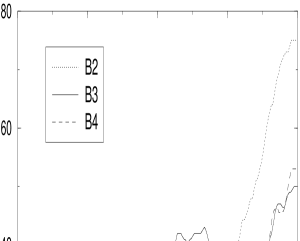
Figure 6: Number of MG stars placed around their nucleus (at a distance $\leq$ 300 pc) as a function of time, for MGs B2, B3 and B4

Figure 7: Position of B2 stars at present and their velocities referred to the LSR and corrected for galactic differential rotation. Different symbols are used for three galactic longitude ranges. The size of the symbols is inversely proportional to the age of the stars they represent

4.3 Older Pleiades subgroups

Groups B3 and B4 in Table 1 are considerably older than B1 and B2, and therefore only few details on the conditions in which they were formed can be recovered. In particular, the uncertainties in $\eta^{\prime}$ due to observational error increase almost monotonically with time. Though this increase can be closely approximated by Eq. 3 for an axysimmetric galactic potential, when considering the terms $\Phi_{\mathrm{Sp}}$ and $\Phi_{\mathrm{B}}$ this approximation breaks (it only works during the first $\approx 10^{8}$ yr). To estimate the effect of typical errors in both the position ($\approx$ 10-15 pc) and velocity ($\approx$ 2-3 km s^-1) components of moving groups on $\eta^{\prime}$ as a function of time, we have simulated a stellar group whose dispersions in the phase space equals those errors, then determined their orbits. We obtain a dispersion in $\eta^{\prime}$ due to these errors of $\approx$ 500 pc after $\sim 3\cdot 10^{8}$ yr. Moreover, we cannot know the way in which individual orbits have been perturbed due to the disc heating effect, producing additional spatial and velocity dispersions.

Figure 8: Stellar trajectories of the B3 members during the last 3.5$\cdot 10^{8}$ yr. The position of the B3 nucleus at $t$ = 0, -1.5 and -3 $10^{8}$ yr (in units of $10^{8}$ yr) is indicated with an open circle. The reference system is the same as in Fig. 3

As mentioned above, these older groups seem to have been born in the vicinity of the spiral arms. The position at birth of groups B3 and B4 are especially interesting: on the one hand, the trajectories followed by these groups show a maximum galactocentric distance at the moment they were born, which corresponds to a minimum kinematic energy (Figs. 3 and 8); on the other hand, by determining the trajectories of the B3 members we observe two focusing points close to the B3 and B4 birthplaces (Fig. 8). An identical result is obtained when using B4 stars. Following Yuan Yuan (1977), these points could be interpreted as the birthplace of B3 and B4. For spatially concentrated groups of stars with small velocity dispersions epicycle theory predicts (Sect. 2) the focusing phenomenon will be produced every $\Delta t=\displaystyle\frac{2\pi}{\kappa}$. Since the Pleiades groups oscillate around a guiding center placed at $R\approx$ 8.0-8.2 kpc, the corresponding epicycle frequency is $\kappa\approx$ 38-40 km s^-1 kpc^-1(determined from $\Phi_{\mathrm{AS}}$, Sect. 3.1), with $\Delta t\approx$ 1.5-1.6 $\cdot 10^{8}$ yr. This period $\Delta t$ is compatible with the ages of B3 and B4.

By following the same procedure used for the B2 group we study the spatial concentration of the older groups (Fig. 6). For B4 there is a maximum concentration at $t\approx-1.5\leavevmode\nobreak\ \cdot 10^{8}$, which corresponds to this MG’s age, whereas we observe two peaks in concentration for B3 at $t\approx-1.5$ and $-3\leavevmode\nobreak\ \cdot 10^{8}$ respectively, the first one corresponding to the last focusing event, and the second one corresponding to the average age of its members.

5 Evolution of a Stellar Complex

As defined by Efremov Efremov (1988), Stellar Complexes (SC) are “groupings of stars hundreds of parsecs in size and up to 10⁸ yr in age, apparently uniting stars born in the same gaseous complex”. Associations and open clusters are the brighter and denser parts of these huge gaseous complexes. In other words, and according to Elmegreen & Elmegreen Elmegreen & Elmegreen (1983), the fundamental unit of star formation is an HI-supercloud of $\sim 10^{7}$ M_⊙ which, during fragmentation into $\sim 10^{5}$-$10^{6}$ M_⊙ giant molecular clouds, gives birth to a SC. From these giant molecular clouds clusters and associations are formed. Examples of SCs are the Gould Belt in our Galaxy, 30 Doradus in the LMC, and NGC 206 in Andromeda.

In this section we explore the possibility that such objects are the progenitors of MGs. Since both galactic differential rotation and disc heating effect tend to disrupt any unbound system of stars on a short timescale, the large number of stars born inside a SC – and therefore roughly sharing the same kinematics and ages – may ensure a high spatial concentration for a longer time, especially at the focusing points.

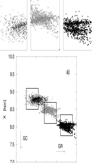
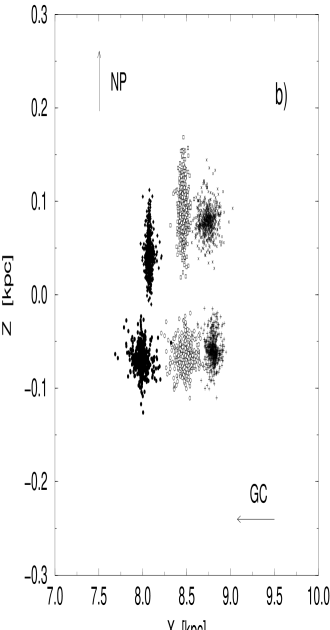
Figure 9: Position on the galactic (a) and meridional (b) planes of the simulated stellar complex at $t=0$ (see text) when no disc heating effect is considered. Three square regions (600 pc/side) on the galactic plane have been enlarged to better distinguish the details. A different symbol is used for each group of stars coming from the same association. GC: galactic center; NP: north galactic pole; GR: galactic rotation

In order to analyse the possible link between SCs and MGs, we have generated a SC as a set of different unbound systems born at different epochs. Its main characteristics are taken from the literature and are described in what follows. Although there are no preferences on the galactic plane region where SCs are formed (they can even be found in the interarm region, as suggested by the observations of OB Associations in Andromeda, e.g. Magnier et al. 1993), we select the position and velocity of the B4 nucleus at birth ($t=-1.5\cdot 10^{8}$ yr), since in this way we can compare the results here obtained with observations on this real group. According to several authors’ estimations Efremov (1988); Elmegreen (1985); Efremov & Chernin (1994), SCs are several hundreds of parsecs in size. The original shape of our simulated complex has been designed as an ellipsoid whose equatorial plane is 250 pc in radius and lies on the galactic plane, and its vertical semi-axis is 70 pc. Six associations are born inside it at different epochs, randomly distributed inside this volume. Since the dispersion in age can be large when considering the SC as a whole Efremov (1988), we impose the condition that one associations borns every 10⁷ yr. Hence, the first one is born at $t=-1.5\cdot 10^{8}$ yr, the second one at $-1.4\cdot 10^{8}$ yr, and so on. The mean velocities of these associations at birth follow a gaussian distribution around the B4 nucleus velocity, with an (isotropic) dispersion similar to the velocity dispersion inside a molecular cloud, i.e. $\approx 5/\sqrt{3}$ km s^-1 in each component Stark & Brand (1989). Each of these associations is defined as follows: they contain 500 stars, which are randomly distributed inside a sphere of 15 pc in diameter, an intermediate value between the smallest associations (e.g. the Trapezium cluster) and the largest ones Blaauw (1991); Brown (1996); and their internal velocity dispersion is 2 km s^-1 in each velocity component, as observed in most of the closer OB Associations Blaauw (1991) and in molecular clouds Scoville (1990); their internal dispersion in ages is 10 ⁷ yr Efremov (1988). We also assume that all the simulated stars survive up to the time ($t$) when we study the system.

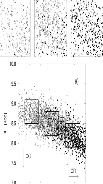
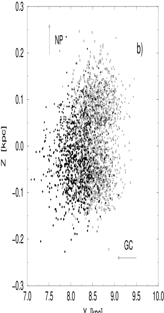
Figure 10: Same as Fig. 9 but considering now the effect of the disc heating on the trajectory of the stars

The orbit of each simulated star from the moment it was born up to the present ($t=0$) is determined considering the galactic gravitational potential ($\Phi_{\mathrm{AS}}+\Phi_{\mathrm{Sp}}+\Phi_{\mathrm{B}}$), without taking into account the disc heating effect. Their current spatial distribution is shown in Fig. 9, where different symbols are used for the stellar “groups” coming from each simulated association. According to our simulation, these groups are still concentrated in space, although their distribution is, at present, far from being isotropic due to the differential rotation. Each of them occupies an ellipsoidal volume $\approx$ 150-250 pc wide, 500 pc long, and 70 pc height, and are perfectly separated in space (four of them can be observed at different positions inside a 300 pc radius sphere around the Sun). The dispersion in each velocity component of any of the groups is still $\approx$ 2 km s^-1, as expected from Eqs. A. Although the mean velocity of these stars is very similar to that of B4, the dispersions in both velocity and space are too small when compared to dispersions in detected MGs that are a few 10⁸ yr old (Table 1). Thus, the spiral arms and central bar perturbations to the galactic gravitational potential cannot account for the observational MGs’ velocity dispersions.

Results drastically change when considering the effect of constant heating on each individual star’s trajectory, as described in Sect. 3.2. To determine these trajectories we use only the axisymmetric part of the galactic potential, since the asymmetric perturbations to this potential are already included in the treatment of the heating. The distribution of the simulated stars at present is shown in Fig. 10. The members of the different groups are now completely mixed with each other. The total SC forms a long structure $\sim$ 3 kpc long and $\sim$ 1 kpc wide. Since in this simulation the Sun has been considered to be in the very center of the SC at $t=0$, the members of this complex can be found up to some 500 pc from us in the radial direction, and much further in the tangential direction. By enlarging a square region (600 pc/side) around the Sun we observe in Fig. 10 that, although the members of two groups dominate in the solar neighbourhood, all the other evolved associations are also represented. Again, the mean velocity components of B4 are recovered when considering only the (636) stars closer than 300 pc from the Sun. However, as expected, the dispersions in velocities are now higher than in the former simulation – the total velocity dispersion is $\approx$ 8-10 km s^-1, depending on the region of the evolved SC. Hence, a constant diffusion of the stellar velocities can perfectly account for B4 velocity dispersions.

In order to study the properties of younger MGs, we analyse the general properties of the complex at its earlier stages, only $5\cdot 10^{7}$ yr after the first association was born. At that moment ($t=-1\cdot 10^{8}$ yr) some stars in the youngest simulated groups are not yet born, while some others are as young as B1 and B2 members. The associations are still very concentrated in the phase space, though some merging can be observed, as happens with B2 group. Velocity dispersions inside each association clearly depend upon their ages, as expected. Thus, in the U-component the velocity dispersion varies from $\approx$ 2.7 km s^-1 for youngest groups to $\approx$ 4.1 km s^-1 for the oldest (in the other components the dispersions are smaller).

Finally, it is interesting to take a look to the general properties of a simulated SC at a larger $t$. The mean properties of the simulated SC are now taken from the B3 nucleus at birth ($t=-3\cdot 10^{8}$ yr). At present ($t=0$ yr), assuming a constant heating of $\sigma_{h}=1.45$ km s^-1 every $\Delta t=10^{7}$ yr, the 3000 simulated stars occupy a huge curved region, about 2 kpc wide and almost 10 kpc long. In the most dense parts of this region, $\sim$ 200 stars can be found in a 300 pc radius sphere, whose total velocity dispersions are very high (12-14 km s^-1). Stars with such large dispersions would be completely merged with field stars, so they could not be detected as MG members. A much smaller diffusion coefficient is needed to recover the B3’s velocity dispersions ($\sigma_{h}\approx 0.7$ km s^-1).

Thus, the disgregation of SCs by means of a constant heating mechanism is not able to account for the whole set of Pleiades MG substructures. A diffusion coefficient that depends on the stellar peculiar velocity and/or on the time (e.g. episodic diffusion) probably might explain the observed properties of these groups. Moreover, the presence of some open clusters in the original SC could keep the stars together in phase space during longer periods. Some young open clusters, i.e. IC 2391, $\alpha$ Persei, Pleiades, etc, share roughly the same kinematics as the groups in Table 1, which favours this hypothesis.

6 Conclusions

In this paper we studied the disruption of unbound systems of stars as a mechanism to understand the origin and evolution of moving groups. The epicycle theory was used to find an analytic expression for the time dependence of dispersion in both the stellar position and velocity coordinates. We have obtained in this way a simple expression for the secular increase of the dispersion in the azimuthal galactic coordinate over time as a function of the initial conditions. This increase in dispersion is, in fact, a direct consequence of the galactic differential rotation.

In order to overtake the constraints of the epicycle theory, we concentrated our analysis on the determination of the stellar trajectories using numerical integration of the equations of motion, which provided us with an independent and more accurate estimation of the evolution of unbound systems. To perform this integration we used an analytic and axisymmetric galactic potential, along with spiral arm and central bar perturbations. This latter procedure allowed us to include random perturbations that mimic the disc heating effect on stellar trajectories.

The trajectories followed by the members of the Pleiades moving group substructures found in Paper I were used to compare the kinematic and photometric ages of these structures, and to establish their position at birth. The youngest group, B1 (the Sco-Cen association), was found to be most spatially concentrated some $9\cdot 10^{6}$ yr ago, a value considerably smaller than its photometric age. This is probably due to the effect of the high stellar atmospheric rotation of early type stars on the observed photometric colors. Groups B4 and B3 were born at a time from the present equal to one and two times the epicycle period respectively, which means that they are spatially focused at present (probably that is the reason why we can observe them). At birth, these two groups were found to be close to the spiral arm structure. Concerning B2, a detailed analysis revealed to us that it is actually composed of several associations which are disintegrating at present. As well, its averaged photometric age is probably overstimated, as in the case of B1.

We considered the evolution of a stellar complex under the influence of the galactic gravitational potential as a mechanism to account for the main physical properties of moving groups. The high velocity dispersions of some of the Pleiades moving group substructures detected among B and A type stars could be recovered when the effect of the disc heating on the individual stellar trajectories was considered. At the same time, the disc heating can account for the mixing of the stellar complex associations, although they are still clearly separated in phase space during the first tens of million years in the complexes’ life (as observed for the groups B1 and B2). After only $1.5\cdot 10^{8}$ yr from the birth of the stellar complex, the complex occupies an ellipsoidal area of $\sim 3\times 1.5$ kpc², with its longest axis oriented in the direction of galactic rotation. If the Sun were presently located in the very center of this disrupted stellar complex, we would be able to find the complex’s components up to very large distances on the galactic plane.

Thus, a constant heating mechanism (compatible with the observational heating law) acting on the stars of a stellar complex can explain the velocity dispersions obtained for those Pleiades moving group substructures that are younger than $\sim 1.5\cdot 10^{8}$. The properties of the older Pleiades substructures could probably be recovered by considering a diffusion coefficient depending on the velocity of the stars, and maybe on the time, and/or the inclusion of open clusters in the simulated stellar complex.

Appendix A Propagation of dispersions with time in the epicycle theory

Let us consider the vector $\@vec{x}$ = ($\xi^{\prime}$,$\eta^{\prime}$,$\zeta^{\prime}$,$\dot{\xi}^{\prime}$,$\dot{\eta}^{\prime}$,$\dot{\zeta}^{\prime}$) containing the position and velocity of a star at a given time $t$. We are interested in determining the propagation of the observational dispersions over time, in the epicycle approximation frame (Eqs. 2, and their derivatives). If we define the vector $\@vec{x}^{\circ}$ = ($\xi^{\prime}_{\circ}$,$\eta^{\prime}_{\circ}$,$\zeta^{\prime}_{\circ}$,$\dot{\xi}^{\prime}_{\circ}$,$\dot{\eta}^{\prime}_{\circ}$,$\dot{\zeta}^{\prime}_{\circ}$) which contains the initial position and velocity of our star, then the initial dispersions can be propagated with time as:

$$\sigma^{2}_{x_{i}}(t)=\displaystyle\sum_{j=1}^{6}\left(\displaystyle\frac{\partial x_{i}(t)}{\partial x_{j}^{\circ}}\right)^{2}_{t}\sigma^{2}_{x_{j}^{\circ}}$$ (12)

where $\sigma_{x_{i}^{\circ}}$ is the observed dispersion in the variable $x_{i}$, and $\sigma_{x_{i}}(t)$ the dispersion at $t$. The dependence of variables $\@vec{x}$ on the initial values $\@vec{x}^{\circ}$ is given by Equations 2. If the coefficients of epicycle equations are included in a vector $\@vec{c}$ = ($\xi^{\prime}_{a}$,$\xi^{\prime}_{b}$,$\eta^{\prime}_{a}$,$\zeta^{\prime}$,$\phi$,$\psi$) then the matrix ${\cal A}=(a^{i}_{j})\equiv\left(\displaystyle\frac{\partial x_{i}}{\partial x_{j}^{\circ}}\right)$ in Equation 12 can be determined as the matrix product ${\cal A}$ = ${\cal B}{\cal F}$, where the matrix ${\cal B}=(b^{i}_{j})\equiv\left(\displaystyle\frac{\partial x_{i}}{\partial c_{j}}\right)$ and ${\cal F}=(f^{i}_{j})\equiv\left(\displaystyle\frac{\partial c_{i}}{\partial x_{j}^{\circ}}\right)$ ($i,j=1,\ldots,6$). By partially differentiating Eqs. 2 we can determine the matrix ${\cal B}$ (Table 4), whereas matrix ${\cal F}$ is determined by just differentiating Eqs. 2 (Table 5). Now, from matrices ${\cal B}$ and ${\cal F}$ we can determine the matrix $\cal A$, given in Table 6. From matrix $\cal A$, and by means of the relationship 12, the propagated dispersions can be expressed as:

Table 4: Elements of the matrix ${\cal B}\equiv\left(\displaystyle\frac{\partial x_{i}}{\partial c_{j}}\right)$ (see text)

$c_{j}$	$x_{i}$
	$\xi^{\prime}$	$\eta^{\prime}$	$\zeta^{\prime}$	$\dot{\xi}^{\prime}$	$\dot{\eta}^{\prime}$	$\dot{\zeta}^{\prime}$
$\xi^{\prime}_{a}$	1	$\cos(\phi+\kappa t)$	0	0	$-\xi^{\prime}_{b}\sin(\kappa t+\phi)$	0
$\xi^{\prime}_{b}$	-2 A $t$	$-\displaystyle\frac{2\omega_{\circ}}{\kappa}\sin(\kappa t+\phi)$	1	0	$-\displaystyle\frac{2\omega_{\circ}\xi^{\prime}_{b}}{\kappa}\cos(\kappa t+\phi)$	0
$\eta^{\prime}_{a}$	0	0	0	$\cos(\nu t+\psi)$	0	$-\zeta^{\prime}_{a}\sin(\nu t+\psi)$
$\zeta^{\prime}$	0	$-\kappa\sin(\kappa t+\phi)$	0	0	$-\xi^{\prime}_{b}\kappa\cos(\kappa t+\phi)$	0
$\phi$	-2 A	$-2\omega_{\circ}\cos(\kappa t+\phi)$	0	0	$2\omega_{\circ}\xi^{\prime}_{b}\sin(\kappa t+\phi)$	0
$\psi$	0	0	0	$-\nu\sin(\nu t+\psi)$	0	$-\nu\zeta^{\prime}_{a}\cos(\nu t+\psi)$

Table 5: Elements of the matrix ${\cal F}\equiv\left(\displaystyle\frac{\partial c_{i}}{\partial x_{j}^{\circ}}\right)$ (see text)

$x_{j}^{\circ}$	$c_{i}$
	$\xi^{\prime}_{a}$	$\xi^{\prime}_{b}$	$\eta^{\prime}_{a}$	$\zeta^{\prime}$	$\phi$	$\psi$
$\xi^{\prime}_{\circ}$	$-\displaystyle\frac{\omega_{\circ}}{\mbox{B}}$	0	0	0	$-\displaystyle\frac{1}{2\mbox{B}}$	0
$\eta^{\prime}_{\circ}$	$\displaystyle\frac{\mbox{A}\cos(\phi)}{\mbox{B}}$	0	0	$-\displaystyle\frac{\sin(\phi)}{\kappa}$	$\displaystyle\frac{\cos(\phi)}{2\mbox{B}}$	0
$\zeta^{\prime}_{\circ}$	0	1	0	$-\displaystyle\frac{2\omega_{\circ}}{\kappa^{2}}$	0	0
$\dot{\xi}^{\prime}_{\circ}$	0	0	$\cos(\psi)$	0	0	$-\displaystyle\frac{\sin(\psi)}{\nu}$
$\dot{\eta}^{\prime}_{\circ}$	$-\displaystyle\frac{\mbox{A}\sin(\phi)}{\xi^{\prime}_{b}\mbox{B}}$	0	0	$-\displaystyle\frac{\cos(\phi)}{\xi^{\prime}_{b}\kappa}$	$-\displaystyle\frac{\sin(\phi)}{2\xi^{\prime}_{b}\mbox{B}}$	0
$\dot{\zeta}^{\prime}_{\circ}$	0	0	$-\displaystyle\frac{\sin(\psi)}{\zeta^{\prime}_{a}}$	0	0	$-\displaystyle\frac{\cos(\psi)}{\nu\zeta^{\prime}_{a}}$

$$\sigma^{2}_{\xi^{\prime}} = \left[\displaystyle\frac{\mbox{A}\cos(\kappa t)-\omega_{\circ}}{\mbox{B}}\right]^{2}\sigma^{2}_{\xi^{\prime}_{\circ}}+\left[\displaystyle\frac{\sin(\kappa t)}{\kappa}\right]^{2}\sigma^{2}_{\dot{\xi}^{\prime}_{\circ}}+$$

$$+\left[\displaystyle\frac{\cos(\kappa t)-1}{2\mbox{B}}\right]^{2}\sigma^{2}_{\dot{\eta}^{\prime}_{\circ}}$$

$$\sigma^{2}_{\eta^{\prime}} = \left[\displaystyle\frac{2\omega_{\circ}\mbox{A}}{\mbox{B}}\left(t-\displaystyle\frac{\sin(\kappa t)}{\kappa}\right)\right]^{2}\sigma^{2}_{\xi^{\prime}_{\circ}}+\sigma^{2}_{\eta^{\prime}_{\circ}}+$$

$$+\left[\displaystyle\frac{2\omega_{\circ}}{\kappa^{2}}\left(\cos(\kappa t)-1\right)\right]^{2}\sigma^{2}_{\dot{\xi}^{\prime}_{\circ}}+$$

$$+\left[\displaystyle\frac{1}{\mbox{B}}\left(\mbox{A}t-\displaystyle\frac{\omega_{\circ}}{\kappa}\sin(\kappa t)\right)\right]^{2}\sigma^{2}_{\dot{\eta}^{\prime}_{\circ}}$$

$$\sigma^{2}_{\zeta^{\prime}} = \cos^{2}(\nu t)\sigma^{2}_{\zeta^{\prime}_{\circ}}+\left[\displaystyle\frac{\sin(\nu t)}{\nu}\right]^{2}\sigma^{2}_{\dot{\zeta}^{\prime}_{\circ}}$$

$$\sigma^{2}_{\dot{\xi}^{\prime}} = \left[\displaystyle\frac{\mbox{A}\kappa}{\mbox{B}}\sin(\kappa t)\right]^{2}\sigma^{2}_{\xi^{\prime}_{\circ}}+\cos^{2}(\kappa t)\sigma^{2}_{\dot{\xi}^{\prime}_{\circ}}+$$

$$+\left[\displaystyle\frac{\kappa}{2\mbox{B}}\sin(\kappa t)\right]^{2}\sigma^{2}_{\dot{\eta}^{\prime}_{\circ}}$$

$$\sigma^{2}_{\dot{\eta}^{\prime}} = \left[\displaystyle\frac{2\mbox{A}\omega_{\circ}}{\mbox{B}}\left(1-\cos(\kappa t)\right)\right]^{2}\sigma^{2}_{\xi^{\prime}_{\circ}}+\left[\displaystyle\frac{2\omega_{\circ}}{\kappa}\sin(\kappa t)\right]^{2}\sigma^{2}_{\dot{\xi}^{\prime}_{\circ}}+$$

$$+\left[\displaystyle\frac{1}{\mbox{B}}\left(\mbox{A}-\omega_{\circ}\cos(\kappa t)\right)\right]^{2}\sigma^{2}_{\dot{\eta}^{\prime}_{\circ}}$$

$$\sigma^{2}_{\dot{\zeta}^{\prime}} = \left[\nu\sin(\nu t)\right]^{2}\sigma^{2}_{\zeta^{\prime}_{\circ}}+\cos^{2}(\nu t)\sigma^{2}_{\dot{\zeta}^{\prime}_{\circ}}\;\mbox{ . }$$ (13)

Table 6: Elements of the matrix ${\cal A}\equiv\left(\displaystyle\frac{\partial x_{i}}{\partial x_{j}^{\circ}}\right)$ (see text)

$x_{j}^{\circ}$	$x_{i}$
	$\xi^{\prime}$	$\eta^{\prime}$	$\zeta^{\prime}$	$\dot{\xi}^{\prime}$	$\dot{\eta}^{\prime}$	$\dot{\zeta}^{\prime}$
$\xi^{\prime}_{\circ}$	$\displaystyle\frac{\mbox{A}\cos(\kappa t)-\omega_{\circ}}{\mbox{B}}$	0	0	$\displaystyle\frac{\sin(\kappa t)}{\kappa}$	$\displaystyle\frac{\cos(\kappa t)-1}{2\mbox{B}}$	0
$\eta^{\prime}_{\circ}$	$\displaystyle\frac{2\omega_{\circ}\mbox{A}}{\mbox{B}}\left[t-\displaystyle\frac{\sin(\kappa t)}{\kappa}\right]$	1	0	$\displaystyle\frac{2\omega_{\circ}}{\kappa^{2}}\left[\cos(\kappa t)-1\right]$	$\displaystyle\frac{1}{\mbox{B}}\left[\mbox{A}t-\displaystyle\frac{\omega_{\circ}}{\kappa}\sin(\kappa t)\right]$	0
$\zeta^{\prime}_{\circ}$	0	0	$\cos(\nu t)$	0	0	$\displaystyle\frac{\sin(\nu t)}{\nu}$
$\dot{\xi}^{\prime}_{\circ}$	$\displaystyle\frac{\mbox{A}\kappa}{\mbox{B}}\sin(\kappa t)$	0	0	$\cos(\kappa t)$	$\displaystyle\frac{\kappa}{2\mbox{B}}\sin(\kappa t)$	0
$\dot{\eta}^{\prime}_{\circ}$	$\displaystyle\frac{2\omega_{\circ}\mbox{A}}{\mbox{B}}\left[1-\cos(\kappa t)\right]$	0	0	$\displaystyle\frac{2\omega_{\circ}}{\kappa}\sin(\kappa t)$	$\displaystyle\frac{1}{\mbox{B}}\left[\mbox{A}-\omega_{\circ}\cos(\kappa t)\right]$	0
$\dot{\zeta}^{\prime}_{\circ}$	0	0	$\nu\sin(\nu t)$	0	0	$\cos(\nu t)$

From these equations we observe that all the dispersions in variables $\@vec{x}$ oscillate around a constant value, except $\sigma^{2}_{\eta^{\prime}}$, whose averaged value increases with time. For small values of $t$ Eqs. A can be approximated by:

$$\sigma_{\xi^{\prime}} \approx \sigma_{\xi^{\prime}_{\circ}}$$

$$\sigma^{2}_{\eta^{\prime}} \approx \sigma^{2}_{\eta^{\prime}_{\circ}}+t^{2}\ \sigma^{2}_{\dot{\eta}^{\prime}_{\circ}}$$

$$\sigma_{\zeta^{\prime}} \approx \sigma_{\zeta^{\prime}_{\circ}}$$

$$\sigma_{\dot{\xi}^{\prime}} \approx \sigma_{\dot{\xi}^{\prime}_{\circ}}$$

$$\sigma_{\dot{\eta}^{\prime}} \approx \sigma_{\dot{\eta}^{\prime}_{\circ}}$$

$$\sigma_{\dot{\zeta}^{\prime}} \approx \sigma_{\dot{\zeta}^{\prime}_{\circ}}\;\mbox{ . }$$

References

- Allen & Santillán (1991) Allen C., Santillán A., 1991, Rev. Mex. Astron. Astrofís. 22, 255
- Asiain et al. (1997) Asiain R., Torra J., Figueras F., 1997, A&A 322, 147
- Asiain et al. (1999) Asiain R., Figueras F., Torra T., Chen B., 1999, A&A 341, 427 (Paper I)
- Becker & Fenkart (1970) Becker W., Fenkart R., 1970, in “The spiral structure of our Galaxy”, W. Becker and G. Contopoulos (eds.), IAU Symp. 38, p.205
- Binney & Lacey (1988) Binney J., Lacey C., 1988, MNRAS 230, 597
- Binney et al. (1991) Binney J., Gerhard O.E., Stark A.A., Bally J., Uchida K.I., 1991, MNRAS 252, 210
- Blaauw (1991) Blaauw A., 1991, in “The Physics of Star Formation and Early Stellar Evolution”, C.J. Lada and N.D. Kylafis (eds.), Kluwer Academic Publishers, p.125
- Blasi (1998) Figueras F., Blasi F., 1998, A&A 329, 957
- Brown (1996) Brown A.G.A., 1996, Stellar content and evolution of OB Associations, PhD Thesis, Thesis Publishers, Amsterdam
- Casertano et al. (1993) Casertano S., Iben I., Jr., Shiels A., 1993, ApJ 410, 90
- Chen et al. (1997) Chen B., Asiain R., Figueras F., Torra J., 1997, A&A 318, 29
- Chereul et al. (1998) Chereul E., Crézé M.,Bienaymé O., 1998, A&A 340, 384
- Comerón et al. (1997) Comerón F., Torra J., Figueras F., 1997, A&A 325, 149
- Efremov (1988) Efremov Y. N., 1988, Soviet Scientific Reviews E., Astrophysics and Space Physics Reviews 7, 105
- Efremov & Chernin (1994) Efremov Y. N., Chernin A.D., 1994, Vistas in Astronomy 38, 165
- Eggen (1989) Eggen O.J., 1989, Fundamental of Cosmic Physics 13, 1
- Eggen (1994) Eggen O.J., 1994, in “Galactic and Solar System Optical Astronomy”, L.V. Morrison, G. Gilmore (eds.). Cambridge University Press, p.191
- Elmegreen (1985) Elmegreen B.G., 1985, in “Birth and Evolution of Massive Stars and Stellar Groups”, W. Boland and H. van Woerden (eds.), p.227
- Elmegreen & Elmegreen (1983) Elmegreen B.G., Elmegreen D.M., 1983, MNRAS 203, 1011
- Fernández (1998) Fernández D., 1998, Tesi de Llicenciatura, Universitat de Barcelona
- Figueras et al. (1997) Figueras F., Gómez A.E., Asiain R., et al., 1997, Hipparcos-Venice’97, ESA SP-402, p.519
- Fridman et al. (1994) Fridman A.M., Khoruzhii O.V., Piskunov A.E., 1994, in “Physics of the Gaseous and Stellar Discs of the Galaxy”, I.R. King (ed.), ASP Conference Series 66, p.215
- Georgelin & Georgelin (1976) Georgelin Y.M., Georgelin Y.P., 1976, A&A 49, 57
- de Geus et al. (1989) de Geuss E.J., de Zeeuw P.T., Lub J., 1989, A&A 216, 44
- Hoogerwerf et al. (1997) Hoogerwerf R., de Bruijne J.H.J., Brown A.G.A., Blaauw A., de Zeeuw P.T, 1997, Hipparcos-Venice’97, ESA SP-402, p.571
- Iben (1967) Iben I., 1967, ARA&A 5, 571
- Kerr & Lynden-Bell (1986) Kerr F.J., Lynden-Bell D., 1986, MNRAS 221, 1023
- Kurtz et al. (1994) Kurtz S., Churchwell E., Wood D.O.S., 1994, ApJS 91, 659
- Lacey (1991) Lacey C., 1991, in “Dynamics of disc galaxies”, Varberg Castle Sweden, p.257
- Lin (1971) Lin C.C., 1971, Theory of spiral structure, Highlights of Astronomy 2, Ed. C. de Jager, Reidel Publ. Co., Dordrecht, Holland, p. 88
- Liszt (1985) Liszt H.S., 1985, Determination of galactic spiral structure at radiofrequencies, in “The Milky Way Galaxy”, IAU Symp. 106, p.283
- Magnier et al. (1993) Magnier E.A., Battinelli P., Lewin W.H.G. et al., 1993, A&A 278, 36
- Mishurov et al. (1997) Mishurov Y.N., Zenina I.A., Dambis A.K., Mel’nik A.M., Rastorguev A.S., 1997, A&A 323, 775
- Mishurov & Zenina (1999) Mishurov Y.N., Zenina I.A., 1999, A&A 341, 81
- Miyamoto & Nagai (1975) Miyamoto M., Nagai R., 1975, PASJ 27, 533
- Miyamoto & Nagai (1975) Miyamoto M., Nagai R., 1975, PASJ 27, 533
- Müllari et al. (1994) Müllari A.A., Nechitailov Yu V., Ninkovic S., Orlov S., 1994, Ap&SS 218, 1
- Palous̆ et al. (1993) Palous̆ J., Jungwiert B., Kopecký J., 1993, A&A 274, 189
- Raboud et al. (1998) Raboud D., Grenon M., Martinet L., Fux R., Udry S., 1998, A&A 335L, 61
- Sabas (1997) Sabas V., 1997, PhD Thesis, Observatoire de Paris
- Sellwood (1999) Sellwood J.A., 1999, PASP 160, 327
- Scoville (1990) Scoville N.Z., 1990, Astr. Society of the Pacific Conf. Ser. 12, p.49
- Sodermblom & Mayor (1993) Soderblom D.R., Mayor M., 1993, AJ 105, 226
- Stark & Brand (1989) Stark A.A., Brand J., 1989, ApJ 339, 763
- Terlevich (1987) Terlevich E., 1987, MNRAS 224, 193
- Theuns (1992) Theuns T., 1992, A&A 259, 503
- Vallée (1995) Vallée J.P., 1995, ApJ 454, 119
- Weidemann et al. (1992) Weidemann V., Jordan S., Iben I., Casertano S., 1992, AJ 104, 1876
- Whitelock & Catchpole (1992) Whitelock P., Catchpole R., 1992, in “The Center, Bulge, and Disk of the Milky Way”, Leo Blitz (ed.), Kluwer Academic Publishers. p.103
- Wielen (1971) Wielen R., 1971, A&A 13, 309
- Wielen (1977) Wielen R., 1977, A&A 60, 263
- Woolley (1960) Woolley R., 1960, Vistas in Astronomy 3, 3. Ed. A.Beer, Pergamon Press, New York
- Yuan (1969) Yuan C., 1969, ApJ 158, 889
- Yuan (1977) Yuan C., 1977, A&A 58, 53
- Yuan & Waxman (1977) Yuan C., Waxman A.M., 1977, A&A 58, 65
- de Zeeuw et al. (1999) de Zeeuw P.T., Hoogerwerf R., de Bruijne J.H.J., Brown A.G.A., Blaauw A., 1999, AJ 117, 354