The LMC eclipsing binary HV 2274: fundamental properties
and comparison with evolutionary models

Abstract

We are carrying out an international, multi-wavelength program to determine the fundamental properties and independent distance estimates of selected 14^th to $15^{\rm th}$ magnitude eclipsing binaries in the Large and Small Magellanic Clouds (LMC and SMC). Eclipsing binaries with well-defined double-line radial velocity curves and light curves provide valuable information on orbital and physical properties of their component stars. These properties include, among other characterisitcs, stellar mass and radius. These can be measured with an accuracy and directness unachievable by any other means. The study of stars in the LMC and SMC where the metal abundances are significantly lower than solar (by 1/3 to 1/10) provides an important opportunity to test stellar atmosphere, interior and evolution models, and opacities. For the first time, we can also measure direct Mass-Luminosity relations for stars outside our Galaxy.

In a previous paper we demonstrated how a precise distance to the LMC — corresponding to $(V_{\circ}-M_{v})_{\rm LMC}=18.30\pm 0.07$ mag — could be determined using the 14^th mag LMC eclipsing binary HV 2274. In this paper we concentrate on the determination of the orbital and physical properties of HV 2274 and its component stars from analyses of light curves and new radial velocity curves formed from HST/Goddard High-Resolution Spectrograph observations. HV 2274 (B1-2 IV-III + B1-2 IV-III; $V_{\rm max}\approx+14.2$; $P=5\fd 73$) is a particularly appealing star because it is a detached binary which has an eccentric orbit ($e=0.136$) and shows fast apsidal motion. The results of these analyses yield reliable masses and absolute radii, as well as other physical and orbital properties of the stars and the system. From UV/optical spectrophotometry ($1150-4820$ Å) of HV 2274 obtained with the HST/Faint Object Spectrograph, the temperatures and the metallicity ($[Fe/H]=-0.45\pm 0.06$) of the stars were found, as well as the interstellar extinction of the system. The values of mass, absolute radius, and effective temperature, for the primary and secondary stars are: $12.2\pm 0.7$ M_⊙, $9.9\pm 0.2$ R_⊙, $23000\pm 180$ K, and $11.4\pm 0.7$ M_⊙, $9.0\pm 0.2$ R_⊙, $23110\pm 180$ K, respectively.

The age of the system ($\tau=17\pm 2$ Myr), helium abundance ($Y=0.26\pm 0.03$) and a lower limit of the convective core overshooting parameter of $\alpha_{\rm ov}\approx 0.2$ were obtained from fitting the stellar data with evolution models of Claret & Giménez. HV 2274 has a relatively well-determined (and fast) apsidal motion period of $U=123\pm 3$ yr. From the analysis of apsidal motion, additional information and constraints on the structure of the stars can be made. The apsidal motion analysis corroborates that some amount of convective core overshooting ($\alpha_{\rm ov}$ between 0.2 and 0.5) is needed.

1 Introduction

Extragalactic eclipsing binaries, and in particular systems belonging to the Large and Small Magellanic Clouds (LMC and SMC), can be used to probe the structure and evolution of stars in environments with chemical histories that differ significantly from those of the solar neighborhood. Studying massive, metal deficient stars in the LMC and SMC is like using a “time machine” for studying the low-metallicity massive old disk O- and B-type stars that once populated our Galaxy about 5-10 billion years ago. In addition, much needed checks of the evolutionary models for these extreme metal abundances, which are widely used in stellar population synthesis calculations, can be performed. LMC and SMC eclipsing binaries can also be used to address other astrophysically — and cosmologically — important issues, such as the structure and dynamics of these galaxies, the enrichment of the interstellar medium, and the distance of the LMC, an important rung on the Cosmic Distance Ladder. General discussions of the importance of extragalactic eclipsing binaries can be found in Graham (1983), Davidge (1987), Koch (1990) and Guinan (1993).

The LMC eclipsing binary HV 2274 ($V_{\rm max}\approx+14.2$) is one of the most interesting and important systems in our current program of LMC and SMC eclipsing binaries (see Guinan et al. 1996, 1998a). HV 2274 is an uncomplicated, detached system consisting of two nearly-identical B1-2 IV-III stars, moving in an eccentric orbit with a period of 5$\fd$73. Moreover, it lies in an uncrowded field, so there is no contamination of the light curves by neighboring stars. $BVI$ light curves have been obtained by Watson et al. (1992, hereafter W92). They modeled the light curves and have determined preliminary values of the photometric, orbital, and geometric properties of the system.

One of the most interesting aspects of HV 2274 is its eccentric orbit, which allows the apsidal motion of the system to be measured. W92 combined recent CCD eclipse timings with older eclipse times estimated from the early photographic photometry and, from this baseline of nearly 60 years, measured an apsidal motion period of U=123$\pm$3 yr. Eclipsing binaries with well-determined apsidal motion rates are important because the internal mass distributions of the stars can be measured (e.g., see Kopal 1959; Guinan 1993). These direct measurements provide extremely important checks on stellar interior and evolution models.

Recently, Guinan et al. (1998b) showed how the combination of light and velocity curve information with UV/optical spectophotometry could yield a precise distance to the HV 2274 system, and thus to the LMC. In this paper, we highlight the properties of the stars themselves and discuss the constraints placed on stellar interiors models through analysis of HV 2274. In §2 the data used in this study are described. §3 is devoted to the modelling of the observational data that leads to the absolute dimensions of the system components. These fundamental properties are compared with the predictions of evolutionary models in §4. The tidal evolution of the system, i.e. synchronization and circularization times, is studied in §5. And, finally, §6 summarizes the main conclusions derived from this work.

2 Observational data

Johnson $BVI$ light curves of HV 2274 were obtained by W92. The observations were made in 1989–1990 from Mount John Observatory (New Zealand) with a 0.61 m telescope equipped with a CCD. Differential photometry in all $BVI$ filters was obtained over 20 nights, with a total number of about 110 measurements in each of the passbands.

HV 2274 was observed with HST as part of a project to obtain UV spectrophotometry of eclipsing binaries in the Magellanic Clouds. Four low-resolution spectra, covering four adjacent wavelength regions, were acquired with HST/FOS (Faint Object Spectrograph). The four spectra were obtained during two successive 96 min. HST orbits, i.e. at essentially the same orbital phase ($\pm 0\@fp 02$). It is important to notice that the studied spectral region contains about 80% of the total flux of the stars. The main characteristics of the spectra are shown in Table 1. The raw data were automatically flux and wavelength calibrated using a set of IDL-based routines prepared by the STScI. The calibration accounted for all the instantaneous information about the spacecraft status, diode problems and instrument response. The data on different wavelength regions were merged (and averaged in the overlapping zones) to produce a single spectrum spanning 1150 Å to 4820 Å which is shown in Fig. 1.

HV 2274 was also selected as a target for a pilot study to secure radial velocity observations with HST so that accurate masses and absolute radii of the stars could be measured. Fourteen spectra were taken at different orbital phases using HST/GHRS (Goddard High-Resolution Spectrograph) in its medium-resolution mode (R=23000, 14 km s^-1/diode, $\Delta\lambda=34$ Å), with integration times $\sim$1100 s and a S/N ratio of about 20. The spectra, whose characteristics are listed in Table 2, cover a wavelength range of 34 Å in two different spectral regions, centered at about $\lambda$1305 Å and $\lambda$1335 Å, where strong UV stellar photospheric lines are typically present for early B-type stars. This fact clearly demonstrates the advantage of UV space-based observations over optical ground-based observations. In the UV domain, numerous photospheric absorption features can be easily identified and used, e.g. Si III, C II, and ionized iron-peak elements. In contrast, in the optical range, even with echelle spectra 3000 Å wide, only a handful of moderately strong He I lines are suitable for obtaining radial velocity measurements.

One of the complete HST/GHRS spectra is shown in Fig. 2 as an example. The spectra taken at orbital conjunction (phases close to 0$\@fp$0 and 0$\@fp$6) were not used for radial velocity determinations since the lines of the components could not be resolved. The spectra contain a number of interstellar lines that are useful for wavelength calibrations.

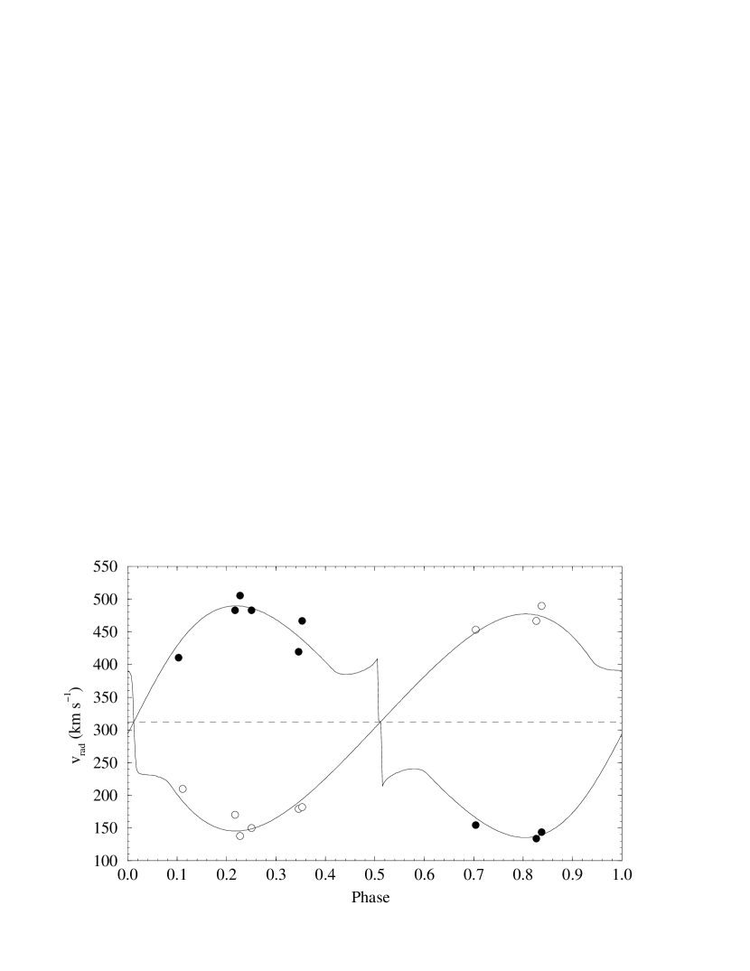
Figure 4: Radial velocity observations of HV 2274 from medium-resolution HST/GHRS spectra (Table 3). The empty circles correspond to the primary component whereas the measurements of the secondary component are represented as filled circles. The best fitting curve was obtained by modeling with WD program. The parameters $e$ and $\omega$ were fixed to the values obtained from the light curve solution. The jumps seen in the model curves, known as “Rossiter effect”, occur when rotating stars are partially eclipsed.

Stellar lines of Fe III at $\lambda$1292.2 Å, Si III (triplet) at $\lambda$1294.5, $\lambda$1296.7 and $\lambda$1298.9 Å, and C II at $\lambda$1323.9 Å were identified in the spectra, as well as several strong ISM lines from both the Milky Way and the LMC. In Fig. 3 we present, as an example, the comparison of two enlarged spectra taken at different phases, with the line identifications included. Several tests were performed to obtain the radial velocity of each component using cross-correlation techniques, but both the small number of usable lines and the strong ISM contamination prevented the obtaining of good results. Instead, double Gaussian fits were applied to derive the exact center of each line for each component and the corresponding radial velocity shift. The continuum level and the intensity, the center and the FWHM of the lines were fitted to the observed spectrum. The fits were, in general, very good. The measurements of different lines in a single spectrum were then averaged to obtain the radial velocity at each phase. The radial velocity measures for each star are listed in Table 3 and are plotted against orbital phase in Fig. 4. The ephemeris of W92 was used to compute the orbital phases. The mean uncertainties in the radial velocity measures are approximately $\pm$15 km s^-1.

3 Analysis and results

All spectroscopic and photometric information was combined to obtain a reliable determination of the orbital, physical and radiative parameters of the system and its components. An iterative procedure was used to achieve internal consistency among the solutions of the light and radial velocity curves and the UV spectrophotometry fit.

3.1 Modeling the light and radial velocity curves

The radial velocity and light curves were both solved simultaneously using an improved Wilson-Devinney program (Wilson & Devinney 1971; Wilson 1979, 1990) that includes the Kurucz (1979) atmosphere model routine developed by Milone et al. (1992, 1994). An automatic procedure was developed in order to keep the WD program running until a solution is found (see Pritchard et al. 1998 for a complete discussion). In this procedure, the computed differential corrections are applied to the input parameters in order to start a new iteration.

The free parameters in the curve fitting were: the eccentricity ($e$), the longitude of the periastron ($\omega$), the phase offset ($\phi_{\circ}$), the inclination ($i$), the temperature of the secondary ($T_{\rm S}$), the gravitational potentials ($\Omega_{\rm P}$ and $\Omega_{\rm S}$), the luminosity of the primary ($L_{\rm P}$), the orbital semi-major axis ($a$), the mass ratio ($q=M_{\rm S}/M_{\rm P}$), and the systemic radial velocity ($\gamma$). Several initial tests done by solving for all orbital, physical and radiative parameters at the same time (light and radial velocity simultaneously), showed clear systematics in the residuals of the light curve because of the small value of the eccentricity indicated by the sparsely covered radial velocity curve. This may also be caused by the fast apsidal motion rate and difference in the epoch of the photometric and radial velocity observations. Due to the correlation, the eccentricity and the longitude of the periastron were derived from the light curve solution alone and held constant in all the subsequent trials. The radial velocity curve and the light curve were analyzed separately and several iterations were performed until reaching a mutually consistent solution.

The fitting of a radial velocity curve is conceptually a simple problem. The free parameters were the orbital semi-major axis ($a$), the mass ratio ($q$) and the systemic velocity ($\gamma$), whereas the eccentricity ($e$) and longitude of the periastron ($\omega$) were set constant to the value given by the light curve solution. We shall remark that $\omega$ was corrected for the epoch difference by using the apsidal motion rate determination of W92. The best fitting curve is shown in Figure 4 and Table 3 lists the individual velocity residuals, which have an rms scatter of 14 km s^-1 and 17 km s^-1 for the primary and secondary components, respectively. The resulting values of the radial velocity curve analysis are included in Table 4. The systemic radial velocity that we obtain, $\gamma=+312$ km s^-1, is in good agreement with the currently adopted value for the heliocentric radial velocity of the LMC galaxy of $+300$ km s^-1. Moreover, the HST/GHRS spectra show strong ISM lines from LMC gas, identified as O I at $\lambda$1302.2 Å and Si II at $\lambda$1304.4 Å, that show only one component with a heliocentric radial velocity of $+285$ km s^-1. The heliocentric radial velocity of the foreground galactic ISM lines was measured to be $-6$ km s^-1.

A detached configuration for the binary (i.e. stars inside their Roche lobes), with coupling between luminosity and temperature was chosen when running the light curve solutions, as suggested by the uncomplicated shapes of the light curve outside the eclipses. Reflection and proximity effects were considered although they are expected to be unimportant for this well-detached system. Both the bolometric albedos and gravity darkening exponents were set to 1.0 as currently adopted for the radiative atmospheres of the components (see Wilson et al. 1972). The mass ratio $q$ was fixed to the spectroscopic value and the temperature of the primary star was set to 23000 K as deduced from the UV/optical spectrophotometry fit (see next section). Finally, the rotational velocities of the components were adopted as $125$ km s^-1 and $115$ km s^-1 (see §3.3).

The $BVI$ light curves were fit simultaneously in order to achieve a single, mutually consistent solution. At each iteration of the automatic procedure, the differential corrections were applied to the input parameters to build the new set of parameters for the next iteration. The result was carefully checked in order to avoid possible unphysical situations (e.g. Roche lobe filling in detached configuration). A solution was defined as the set of parameters for which the differential corrections suggested by the WD program were smaller than the standard errors during three consecutive iterations. However, when a solution was found, the program did not terminate. Instead, it was kept running in order to test the stability of the solutions, to evaluate their scatter, and to check for possible spurious solutions.

In the modeling of the light curves of eccentric systems, there exist two different sets of parameters that provide almost identical fits to the observations. For HV 2274, the first one has a more massive star which is larger and cooler than the less massive star, whereas in the other solution, the more massive component is smaller and hotter. There is not sufficient information in the light or radial velocity curves to discriminate between these two possible solutions, and other data sources have to be considered to break this degeneracy. Since the luminosity ratio between the components predicted by the two solutions is very different ($L_{\rm S}/L_{\rm P}\approx 0.85$ and $L_{\rm S}/L_{\rm P}\approx 1.2$), we measured the equivalent widths of several pairs of lines in the GHRS spectra to estimate the spectroscopic light ratio of the two stars. We obtained a mean value of $0.88\pm 0.05$, which, given the nearly identical temperatures of the stars, clearly indicates that the first solution is the physically preferable one.

The best fitting parameters are shown in Table 4. With such parameters, the rms scatters of the residuals are 0.018 (n=108), 0.013 (n=116) and 0.019 mag (n=112) for $BVI$ respectively. Fig. 5 shows, as an example, the light curve fit to the observed $V$ differential photometry and the corresponding residuals. The uncertainties in the light curve parameters were carefully evaluated and adopted as three times the rms scatter of a set of several solutions obtained from different initial conditions, instead of the formal standard errors computed by the WD program. This approach provides more realistic estimations of the actual uncertainties of the computed properties.

W92 also attempted a preliminary solution of their observed light curves by using the EBOP program (Etzel 1975, 1993). Since they had no information about the mass ratio ($q$) or the radius ratio ($k$), only the orbital parameters $e$, $i$ and $\omega$, that are essentially insensitive to $q$ and $k$, were explicitly listed by the authors. When comparing our results with their initial estimations we find agreement within the quoted errors.

3.2 Modeling the spectrophotometry

The spectrophotometric analysis consisted of finding the pair of ATLAS9 atmosphere models (Kurucz 1991, 1994) which best reproduces the observed energy distribution of the HV 2274 system (FOS data plus $B-V$). The $B$ and $V$ calibrated photometry outside the eclipses was taken from the photometric measurements of Udalski et al. (1998). The photometry of W92 was not used because of its poorer accuracy ($\approx 0.1$ mag), as pointed out by the authors themselves.

Each ATLAS9 model is characterized by four parameters: effective temperature ($T_{\rm eff}$), surface gravity ($\log g$), metalicity ($[m/H]$) and microturbulence velocity ($\mu$). A non-linear least squares algorithm developed by Fitzpatrick & Massa (1999) was employed to find the combination of model parameters — along with the appropriate interstellar extinction curve — which best reproduce the observations. The technique is discussed in detail in Fitzpatrick & Massa (1999), but, in short, this approach is feasible because the signatures of interstellar extinction, temperature, surface gravity, metallicity and microturbulence in the model spectrum are very different from each other. The fitting algorithm also evaluates the 1$\sigma$ internal errors that account for the full interdependence of all the parameters.

The eight possible parameters describing the HV2274 models are heavily constrained by the results of the light and radial velocity curve analysis, which yielded values of the surface gravity of each component and the ratio of the effective temperatures. As additional constraints we assumed that the two stars in the system have identical metallicity and microturbulence velocity.

The best fitting model to HV2274 is shown in Fig. 6 and Table 4 summarizes the derived properties, together with their errors. The shape of the UV interstellar extinction curve, derived via the fitting procedure, shows a much weaker 2175 Å extinction bump than found along typical Milky Way lines of sight. The properties of the UV extinction curves seen towards Magellanic Cloud eclipsing binaries will be discussed in a future paper. To investigate the validity of the ATLAS9 models and, thus, the physical significance of the derived quantities, we performed a second fit by constraining only the difference in surface gravities between the components but not the actual $\log g$ values. This resulted in a value of $\log g=3.51\pm 0.05$ dex for the primary component, gratifyingly close to the result based on the orbital solution alone. In addition, the metal abundance from the FOS spectrum fit, $[Fe/H]=-0.45\pm 0.06$ dex with respect to solar abundances, is in good agreement with the metal abundances typically reported for the LMC ($\sim$ $-0.5$, $-0.6$ dex; Bica et al. 1998). These results strengthen our confidence in the determination of the remaining parameters.

3.3 Rotational velocity

Apart from obtaining a radial velocity curve, the HST/GHRS spectra were used to estimate the rotational velocity of the components. An accurate measurement was not possible due to the lack of spectra of standard stars, but an estimation could be done by comparing the observations with synthetic spectra. When building the synthetic spectra, we adopted ATLAS9 models and the set of programs developed by I. Hubeny (synspec, rotin and synplot), which were modified to combine, in the correct proportion, the flux of both components (see Ribas et al. 1999). Atmosphere models with $\log~{}g=3.5$ dex were used. The effective temperature of each component, the microturbulence velocity and the metalicity were fixed from the results of the spectrophotometry fit.

The rotational velocities of the components, the only free parameters, were interactively changed until the best possible agreement between the observed and the synthetic spectra was reached. The profiles of the same lines used for radial velocity measures (mentioned in §2) were employed during this procedure. The best fit to the observed spectrum was obtained when considering rotational velocities of $125$ km s^-1 and $115$ km s^-1 for the primary and secondary components, respectively. The error of these values is estimated to be around $10$ km s^-1. The pseudo-synchronization velocities (i.e. synchronization at periastron) for the components of HV 2274 are $117$ km s^-1 and $107$ km s^-1, both within the error bars of our estimates. Therefore, we conclude that both components are synchronized with the orbital velocity at periastron.

4 Comparison with Evolutionary Models

A comparison of the derived physical properties of the stars with the theoretical predictions of stellar evolutionary models was also made. We considered the evolutionary models of Claret (1995, 1997) and Claret & Giménez (1995, 1998) (altogether referred to as CG). These models cover a wide range in both metalicity ($Z$) and initial helium abundance ($Y$), incorporate the most modern input physics and adopt a value of 0.2 H_p as the overshooting parameter ($\alpha_{\rm ov}$). An identical set of models that consider no convective overshoot was kindly provided by A. Claret (priv. comm.).

The stellar evolutionary models were interpolated at a metal abundance of $Z=0.007$, as suggested by the results of the FOS spectrum fit. Once the metalicity is fixed and the masses, radii and effective temperatures of the components are known, the only free parameter in the the adopted set of evolutionary models is the initial helium abundance $Y$. A simple least squares procedure indicated that the value of the initial helium abundance that best reproduces the current properties of HV 2274 components is $Y=0.26$. After several more trials taking into account the uncertainties in masses, radii and effective temperature, we estimated the uncertainty of this quantity to be around $\pm 0.03$. The main source of error in the determination of $Y$ is the uncertainty in the masses, but nevertheless, the good accuracy of the estimation, $Y=0.26\pm 0.03$, is noteworthy. This value of $Y$ shows a very good agreement with the expected helium abundance from the currently adopted chemical enrichment law (see Izotov & Thuan 1998).

The parameters yielded by the evolutionary models using the derived chemical composition are listed in Table 5. As observed, good agreement is obtained for the temperatures and the ages of both components. The evolutionary age of the system can be placed around 17.5 Myr. Also, notice that the stars have lost about 1% of their initial mass via stellar winds. The location of both components of HV 2274 is shown in the $\log g-\log T_{\rm eff}$ plot (Fig. 8). Also shown in this figure are the evolutionary tracks at $Z=0.007$ and $Y=0.26$ for the ZAMS masses of the components and the isochrone that provides the best fit to the system. The agreement between the theoretical and observed stellar properties are well within the observational errors. It is also evident from the plot that the two stars are rather evolved and close to the terminal age main-sequence (TAMS).

Unfortunately, HV 2274 is not a very suitable object for a detailed study of the effects of overshooting through isochrone fitting, since both components are very similar. This means that, as long as both stars lie within the main sequence, it is always possible to find an initial helium abundance that reproduces the observed properties of the components. There exists no possibility of discriminating between different overshooting parameters since their effect is small inside the main sequence and also it is very similar for both components (small “zero point” changes but no “differential effect”).

However, in the case of $\alpha_{\rm ov}<0.2$, both components are located beyond the TAMS. In such a situation, the evolution of the stars is so fast that, unless they have almost identical mass, their effective temperatures should be significantly different (at the same age). This is in disagreement with the results of the analysis of the light curves and the UV spectrophotometry. Moreover, a mass ratio of unity is not compatible with the radial velocity curve solution. We show in Figure 9 a $\log g-\log T_{\rm eff}$ of HV 2274 with the corresponding evolutionary tracks and best-fitting isochrone for $\alpha_{\rm ov}=0$ for $Y=0.26$ (as for $\alpha_{\rm ov}=0.2$, this value is the one that best reproduces the observed temperatures).

Stellar lifetime considerations can also be considered. Actually, straightforward calculations using evolutionary model tracks show that, for the masses of HV 2274 components, less than 1% of the stellar lifetime is spent beyond the TAMS. This implies that it is very unlikely to observe both components of a binary system in the rapid evolving stage beyond the main sequence. The argument constitutes additional evidence favoring evolutionary models with an overshooting parameter larger than 0.2, which predict both components to be located within the main sequence. For lower overshooting parameters, both components are predicted to lie in the Hertzsprung gap of the H-R diagram.

From all the previous evidences, an overshooting parameter below 0.2 can be confidently ruled out. This result is especially valuable since it is the first test of the significance of overshooting that has been made for stars of such low metal abundance.

A parallel test of stellar structure and evolution models can also be performed, since HV 2274 has an eccentric orbit and W92 have determined its apsidal motion rate. The apsidal motion rate of a binary system can be theoretically computed as the linear sum of a general relativity term (GR) and a classical term (CL). The latter, which is the most important contribution in close systems like HV 2274, depends on the internal mass distribution of the stars ($k_{2}$), which can also be theoretically estimated from the evolutionary models. Linear interpolation in the CG models provides the values for $\log{k_{2}}$ shown in Table 5. These values were corrected for stellar rotation by means of the formula of Claret & Giménez (1993). With this correction, $\Delta\log{k_{2}}_{\rm P,S}=-0.03$, the internal concentration parameters are $\log{k_{2}}_{\rm P}=-2.46\pm 0.02$ and $\log{k_{2}}_{\rm S}=-2.43\pm 0.02$, which lead to a mean system value of $\log{\overline{k}_{2}}=-2.45\pm 0.02$. Also using the formulas in Claret & Giménez (1993), we derive a total theoretical apsidal motion rate of $\dot{\omega}{\rm(th)}=3.06\pm 0.30$ deg/yr, in which ${\dot{\omega}}_{\rm CL}=2.97$ deg/yr is the classical term and ${\dot{\omega}}_{\rm GR}=0.09$ deg/yr is the general relativistic contribution. When comparing the theoretical determination with the observed value, $\dot{\omega}{\rm(obs)}=2.93\pm 0.07$ deg/yr, we find a remarkable agreement. The results of the apsidal motion study are summarized in Table 6.

The internal concentration of a star is strongly influenced by the convection parameters adopted for the stellar cores, in particular $\alpha_{\rm ov}$, but weakly dependent on the chemical composition (for a given set of convection parameters). In general, a larger overshooting means a higher internal concentration, since the star can remain a longer time on the main sequence. From the study of V380 Cyg (Guinan et al. 1999) and the paper by Claret & Giménez (1993) it can be deduced that, for the masses and evolutionary stage of HV 2274, an increasing of the overshooting parameter of $\Delta\alpha_{\rm ov}=0.1$ implies a decreasing of $\Delta\log k_{2}=-0.02$, with a good linear behavior. Taking into account this crude approximation and the $1\sigma$ uncertainties of the absolute dimensions, it is inferred that the observed apsidal motion rate is only reproduced if $0.1<\alpha_{\rm ov}<0.5$. Although the formal best fit is obtained for $\alpha_{\rm ov}=0.3$.

The overall conclusion that can be reached from the comparison of the observed properties with stellar evolutionary models is that the overshooting parameter that best reproduces the observations can be constrained between $0.2<\alpha_{\rm ov}<0.5$. The constraint was possible by combining the analysis of the positions in the theoretical H-R diagram (lower limit) and the study of the apsidal motion rate (upper limit). We have to stress that this result is valid only for the component masses of HV 2274 and for the chemical composition of the system, $Z=0.007$ and $Y=0.26$. V380 Cyg (Guinan et al. 1999) is a solar composition system ($Z=0.02$, $Y=0.28$) with a primary component of very similar mass to that of the components of HV 2274 (within 10%). However, the overshooting parameter needed for reproducing observed properties of V380 Cyg is larger (and better constrained) than the value that we have found for HV 2274. Since a mass effect is ruled out, the only possible explanations are either an overshooting parameter variable (increasing) with evolution or a chemical composition effect. Both possibilities have interesting consequences and deserve further study.

5 Tidal Evolution

The observations show that the components of HV 2274 are moving in an eccentric orbit and that they appear to have rotational velocities synchronized with the orbital velocity at periastron. This is a common situation since in most cases the circularization timescale is much larger than the synchronization timescale. In order to compare this with the theoretical predictions, we adopted the tidal evolution formalism of Tassoul (1987, 1988). The mathematical expressions, which were taken from Claret et al. (1995), relate the time variation of the eccentricity and the angular rotation with the orbital and stellar physical properties: mass ratio, orbital period, mass, luminosity, radius and gyration radius. We stress the importance of integrating the differential equation that governs the variation with time of the eccentricity and the angular velocity rather than a simple timescale calculation (linear approximation). This is especially advisable for evolved systems like HV 2274, since the components undergo strong radius and luminosity changes.

We therefore integrated the differential equations along evolutionary tracks for the ZAMS masses of the HV 2274 components. The orbital period was assumed to be constant during the integration. As contour conditions, we imposed the eccentricity to be the observed value ($e=0.136\pm 0.012$) at the present age of the system ($\tau=17.5\pm 2.5$ Myr). Also, the angular rotation was normalized to unity at the ZAMS. The calculations were done with the evolutionary models at $Z=0.007$ and $Y=0.26$. As expected, the theoretical predictions indicate a system that has reached synchronism but that has not yet circularized its orbit. Indeed, both components reduced the difference between their angular velocity and the pseudo-synchronization angular velocity to less 0.1% of the ZAMS value at the early age of 2 Myr. From the contour condition it is inferred that the ZAMS orbital eccentricity was quite large ($e_{\rm ZAMS}\approx 0.7$), and thus it has undergone a noticeable decreasing from this initially high value. The theory also predicts that the circularization will take place as soon as the primary component increases significantly its radius shortly after the onset of the shell hydrogen burning. The actual time, however, depends on the amount of convective overshooting, which affects the position of the TAMS.

6 Conclusions

This paper demonstrates clearly that the study of extragalactic eclipsing binaries is now feasible and can lead to some interesting and important results on the properties and evolution for stars outside of our Galaxy. Also, as shown in our first paper, eclipsing binaries can serve as excellent “standard candles” for calibrating the distance to the LMC and in the near future, the Andromeda Galaxy. Remarkably, less than ten years ago there were fewer than 150 extragalactic eclipsing binaries known, with most of these being members of the LMC, SMC and M31. However, this picture has drastically changed with the serendipitous discovery of thousands of new extragalactic eclipsing binaries from mainly the OGLE and MACHO microlensing surveys. For example, today there are nearly as many eclipsing binaries known in the LMC (2500) than cataloged in the Milky Way itself (about 3000). In fact, it is estimated that a total of about 8000 eclipsing binaries will probably be discovered in the LMC from the MACHO program when it is completed (Cook 1999).

The large number of eclipsing binary systems provides a wide variety of systems and stars to choose for further study. To get the maximum scientific returns from these stars, however, requires considerable effort, mainly because high quality light curves and radial velocity curves are essential to extract the fundamental astrophysically important information from these systems. Moreover, calibrated spectroscopy or spectrophotometry (as was used here from HST), or standardized $UBVRI$ or well-calibrated Strömgren $uvby$ photometry, as well as high-dispersion spectroscopy are needed to determine the temperatures and metalicities of the stars and also to determine interstellar reddening and extinction needed for distances and modeling. Although it takes a lot of work, none of the needed observations is beyond current instrumental capabilities. Good-quality light curves of 14^th and 15^th mag systems can routinely be done with 1-m aperture telescopes. Spectroscopic observations of these same stars (for radial velocity, temperature and abundance studies), however, need to be done with 4-m class telescopes or, more efficiently, from space with HST using STIS.

In addition to HV 2274, we have secured HST/FOS spectra covering $1150-4820$ Å for nine other LMC and SMC eclipsing systems with components having late O and early B spectral types. The systems with FOS spectra are HV 982, HV 1620, HV 1761, HV 1876, HV 2226, HV 2241, HV 5936, HV 12634 and EROS 1044. We also have IUE FUV spectra for a several other LMC eclipsing binaries. Most of these systems have light curves but lack satisfactory radial velocity curves. We have recently submitted requests for time on the 4-m CTIO telescope and plan to submit a proposal to the HST later this year for STIS observations.

In the near future we hope to revisit HV 2274 when better light and radial velocity curves become available. Improved masses, stellar radii and distances are possible with more observations. It may be somewhat strange that the properties of this faint LMC system are better determined than most eclipsing binaries in our own Galaxy. This situation arises mainly because very few eclipsing binaries in our Galaxies have FOS spectrophotometry from which accurate temperatures can be derived. Also, HV 2274 is an interesting target for high-precision photometry since the component stars lie near the locations in the H-R diagram in our Galaxy where $\beta$ Canis Majoris variables are located. It would be interesting to conduct more extensive photometry to see if light variations from pulsations of the stars can be found. If short-term (several hours) light variations are discovered, then HV 2274 could be a prime candidate for a detailed asteroseismology study. In this case, the eclipses could be used to isolate the star or stars that pulsate.

Table 1: HST/FOS spectra of HV 2274 in four different wavelength regions obtained on 1996 November 15, when the eclipsing binary was near quadrature ($\phi=0\@fp 22$). In this situation, the combined flux of both components is observed.

Range (Å)	res. (Å/bin)	$t_{\rm int}$ (sec)	S/N
1140–1620	1.0	920	25
1550–2350	1.6	680	30
2220–3300	2.2	600	50
3210–4820	3.2	680	40

Table 2: HST/GHRS medium-resolution spectra of HV 2274.

Nr.	HJD-2450000	Phase	$\lambda$ (cent.)
1	402.9159	0.2172	1335
2	402.9733	0.2272	1300
3	413.0330	0.9840	1335
4	413.0689	0.9903	1300
5	413.7106	0.1024	1335
6	413.7589	0.1108	1300
7	416.5881	0.6049	1335
8	416.6324	0.6126	1300
9	417.1551	0.7039	1335
10	417.8555	0.8263	1335
11	417.9199	0.8375	1300
12	420.2828	0.2501	1335
13	420.8290	0.3455	1335
14	420.8702	0.3527	1300

Table 3: Radial velocity measurements of HV 2274 from HST/GHRS medium-resolution spectra. The mean errors are about 15 km s^-1. Wt. is the relative weight assigned to each measurement. O$-$C is the residual in the radial velocity curve fit.

P component					S component
HJD$-$	$v_{\rm r}$	Wt.	O$-$C		HJD$-$	$v_{\rm r}$	Wt.	O$-$C
2450000	(km s-1)		(km s-1)		2450000	(km s-1)		(km s-1)
402.91589	170.3	0.5	24.9		402.91589	482.8	1.0	$-$7.0
402.97328	137.9	0.5	$-$7.8		402.97328	505.4	1.0	15.9
413.75888	210.2	1.0	19.0		413.71058	410.3	1.0	$-$20.1
417.15507	453.3	1.0	4.8		417.15507	154.4	1.0	$-$11.5
417.85554	466.9	1.0	$-$8.4		417.85554	134.1	0.5	$-$3.9
417.91995	489.6	1.0	16.4		417.91995	143.8	1.0	3.4
420.28279	149.9	0.5	1.1		420.28279	482.8	0.5	$-$3.6
420.82902	179.3	1.0	$-$10.4		420.82902	419.4	1.0	$-$23.5
420.87019	182.0	1.0	$-$12.1		420.87019	466.7	1.0	28.4

Table 4: Orbital and stellar properties of HV2274 derived from the analysis of the light and radial velocity curves and the FOS spectrum fit. The numbers in parentheses are the standard errors affecting the last digits of each parameter. Subscripts P and S refer to the primary and secondary components, respectively.

Light curve solution
$P=5.726006(12)$ days	$e=0.136(12)$	$\left.\frac{L_{\rm S}}{L_{\rm P}}\right|_{B}=0.845(5)$
$i=89\fdg 6(1.3)$	$\omega(1990.6)=73\fdg 3(1.5)$	$\left.\frac{L_{\rm S}}{L_{\rm P}}\right|_{V}=0.844(5)$
$r_{\rm P}=0.255(2)$	$\dot{\omega}=2.93(7)$ deg/yr	$\left.\frac{L_{\rm S}}{L_{\rm P}}\right|_{I}=0.843(5)$
$r_{\rm S}=0.234(2)$	$\frac{{T_{\rm eff}}_{\rm S}}{{T_{\rm eff}}_{\rm P}}=1.005(5)$
Radial velocity curve solution
$K_{\rm P}=166.2(5.9)$ km s-1	$q=\frac{M_{\rm S}}{M_{\rm P}}=0.938(45)$	$\gamma=312(4)$ km s-1
$K_{\rm S}=177.3(5.8)$ km s-1	$a=38.58(93)$ R☉
UV/Optical spectrophotometry
${T_{\rm eff}}_{\rm P}=23000(180)$ K	$[Fe/H]=-0.45(6)$ dex	$E(B-V)=0.120(9)$
${T_{\rm eff}}_{\rm S}=23110(180)$ K	$\mu_{\rm PS}=1.9(7)$ km s-1
Stellar physical properties
$\begin{array}[]{lll}M_{\rm P}=12.2(7)~{}{\rm M}_{\odot}&\mbox{\hskip 56.9055pt}&M_{\rm S}=11.4(7)~{}{\rm M}_{\odot}\\ R_{\rm P}=9.86(24)~{}{\rm R}_{\odot}&&R_{\rm S}=9.03(24)~{}{\rm R}_{\odot}\\ \log g_{\rm P}=3.536(27)~{}{\rm dex}&&\log g_{\rm S}=3.585(29)~{}{\rm dex}\\ {T_{\rm eff}}_{\rm P}=23000(180)~{}{\rm K}&&{T_{\rm eff}}_{\rm S}=23110(180)~{}{\rm K}\\ \overline{\rho_{\rm P}}=0.018(2)~{}\mbox{g cm${}^{-3}$}&&\overline{\rho_{\rm S}}=0.022(2)~{}\mbox{g cm${}^{-3}$}\\ {\rho_{\rm c}}_{\rm P}\tablenotemark{a}=4.2(6)~{}\mbox{g cm${}^{-3}$}&&{\rho_{\rm c}}_{\rm S}\tablenotemark{a}=4.8(7)~{}\mbox{g cm${}^{-3}$}\\ {v_{\rm rot}}_{\rm P}=125~{}\mbox{km s${}^{-1}$}&&{v_{\rm rot}}_{\rm S}=115~{}\mbox{km~{}s${}^{-1}$}\end{array}$
Distance determination
$\begin{array}[]{lll}d_{\rm HV2274}=46.8(1.6)~{}{\rm kpc}&&V_{\circ}-M_{v}=18.35(7)~{}{\rm mag}\\ d_{\rm LMC}=45.7(1.6)~{}{\rm kpc}&&V_{\circ}-M_{v}=18.30(7)~{}{\rm mag}\end{array}$

Table 5: Results of a linear interpolation in the CG models that consider $\alpha_{\rm ov}=0.2$. The input parameters are the observed absolute dimensions of HV 2274 and a chemical composition of $Z=0.007$ and $Y=0.26$.

	P comp.	S comp.
$T_{\rm eff}$ (K)	$23260\pm 680\hskip 3.0pt$	$22940\pm 730\hskip 3.0pt$
$Age$ (Myr)	$16.7\pm 1.6\hskip 6.0pt$	$18.3\pm 1.9\hskip 6.0pt$
$\log(L/L_{\odot})$	$4.40\pm 0.07$	$4.30\pm 0.08$
$\log k_{2}$	$-2.43\pm 0.02$	$-2.40\pm 0.02$
$M_{\rm ZAMS}$ (M☉)	$12.37\pm 0.72$	$11.53\pm 0.72$

Table 6: Summary of results of the apsidal motion study of HV 2274. Evolutionary models of CG with $\alpha_{\rm ov}=0.2$, $Z=0.007$ and $Y=0.26$ were used for the theoretical calculations. The superscript r means that the rotational correction has been applied ($\Delta\log{k_{2}}_{\rm P,S}({\rm rot.})=-0.03$).

Apsidal motion
$\left.\begin{array}[]{l}\log{k_{2}}^{\rm r}_{\rm P}({\rm th})=-2.46(2)\\ \log{k_{2}}^{\rm r}_{\rm S}({\rm th})=-2.43(2)\end{array}\right\}\Longrightarrow\log{{\overline{k}}_{2}}^{\rm r}({\rm th})=-2.45(2)$
$\left.\begin{array}[]{l}{\dot{\omega}}_{\rm CL}=2.97(30)\;{\rm deg/yr}\\ {\dot{\omega}}_{\rm GR}=0.09(0)\;{\rm deg/yr}\end{array}\right\}\Longrightarrow\dot{\omega}({\rm th})=3.06(30)\;{\rm deg/yr}$
$\dot{\omega}({\rm obs})=2.93(7)\;{\rm deg/yr}$

Figure 1: Full observed HST/FOS spectrum of HV 2274 (5-point smoothing filter applied).

Figure 2: HST/GHRS spectrum of HV 2274 centered at the $\lambda$1300 Å region (spectrum Nr. 12 in Table 2). The strongest features in the spectrum are ISM absorption lines from both our Galaxy (MW) and the LMC. The lines are labeled with the ion identification and the rest wavelength.

Figure 3: HST/GHRS spectra of HV 2274. The upper panels show two spectra taken at phases 0$\@fp$99 and 0$\@fp$98 (during primary eclipse, spectra Nr. 4 and 3 of Table 2) where single lines of Fe III, Si III (triplet) and C II are identified. The spectra shown in the lower panel were taken at phases 0$\@fp$84 and 0$\@fp$35 (spectra Nr. 11 and 13 of Table 2), and the lines corresponding to the primary (P) and secondary (S) components are observed, though in some cases (Si III triplet) they overlap.

Figure 5: Light curve fit to the observed $V$ Variable$-$Comparison (V$-$Cp) differential photometry of W92. Also shown are the Observed$-$Computed (O$-$C) residuals. The orbital phase is computed according to the linear ephemeris $\mbox{Min I (HJD)}=2448099.818+5.726006\,E$.

Figure 6: The UV/optical energy distribution of HV 2274, in units of erg cm^-2 s^-1 Å^-1. The lower full spectrum shows the observed HST/FOS energy distribution; the upper spectrum shows the extinction-corrected energy distribution, superimposed with the best-fitting ATLAS9 atmosphere model (plotted in histogram style). Vertical lines through the data points indicate the 1$\sigma$ observational errors. Crosses indicate data points excluded from the fit due to contamination by interstellar absorption lines. The large filled circles show the dereddened B and V photometry from Udalski et al. (1998). An expanded view of the fit near the Balmer jump is shown within the inset.

Figure 7: 3-D picture of HV 2274 in quadrature phase.

Figure 8: $\log g-\log T_{\rm eff}$ plot of HV 2274 (P stands for primary component and S for secondary component). The evolutionary tracks and isochrones were computed from the evolutionary models of CG that consider $\alpha_{\rm ov}=0.2$ and with $Z=0.007$ and $Y=0.26$. Mass loss has been taken into account when computing the evolutionary tracks. The error bars in the symbols only consider the “differential” effect in $\Delta\log g$ and $\Delta\log T_{\rm eff}$ (see text). The complete error budget is shown in the right part of the diagram. A blowup of the region where the stars are located is shown within the inset.

Figure 9: Same as Figure 8 but for the evolutionary models of CG that consider $\alpha_{\rm ov}=0$.

References

- Bica et al. (1998) Bica, E., Geisler, D., Dottori, H., Clariá, J. J., Piatti, A. E., & Santos, J. F. C.,Jr. 1998, AJ 116, 723
- Claret (1995) Claret, A. 1995, A&AS, 109, 441
- Claret (1997) Claret, A. 1997, A&AS, 125, 439
- Claret & Giménez (1993) Claret, A., & Giménez, A. 1993, A&A 277, 487
- Claret & Giménez (1995) Claret, A., & Giménez, A. 1995, A&AS, 114, 549
- Claret & Giménez (1997) Claret, A., & Giménez, A. 1998, A&AS, 133, 12
- Claret et al. (1995) Claret, A., Giménez, A., & Cunha, N. C. S. 1995, A&A 299, 724
- Cook (1999) Cook, K. 1999, private communication
- Davidge (1987) Davidge, T. J. 1987, AJ 94, 1169
- Etzel (1975) Etzel, P. B. 1975, Masters Thesis, San Diego State University
- Etzel (1993) Etzel, P. B. 1993, in Light Curve Modelling of Eclipsing Binary Stars, ed. E. F. Milone, Springer-Verlag, Berlin, p. 113
- Fitzpatrick & Massa (1999) Fitzpatrick, E. L., & Massa, D. 1999, in preparation
- Graham (1983) Graham, J. A. 1983, Highlights of Astronomy 6, 209
- Guinan (1993) Guinan, E. F. 1993, in New Frontiers in Binary Star Research, eds. K. C. Leung & I. S. Nha, A. S. P. Conf. Series, vol. 38, p. 1
- Guinan et al. (1996) Guinan, E. F., Bradstreet, D. H., & DeWarf, L. E. 1996, in The Origins, Evolutions, and Destinies of Binary Stars in Clusters, eds. E. F. Milone & J. -C. Mermilliod, A. S. P. Conf. Series, vol. 90, p. 197
- Guinan et al. (1998a) Guinan, E. F., Ribas, I., Fitzpatrick, E. L., & Pritchard, J. D. 1998a, in Ultraviolet Astrophysics beyond the IUE final archive, eds. W. Wamsteker & R. González-Riestra, ESA SP-413, p. 315
- Guinan et al. (1998b) Guinan, E. F., Fitzpatrick, E. L., DeWarf, L. E., Maloney, F. P., Maurone, P. A., Ribas, I., Giménez, A., Pritchard, J. D., & Bradstreet, D. H. 1998b, ApJ 509, L21
- Guinan et al. (1999) Guinan, E. F., Ribas, I., Fitzpatrick, E. L., Giménez, A., Bradstreet, D. H., & Popper, D. M. 1999, in preparation
- Izotov & Thuan (1998) Izotov, Y. I., & Thuan, T. X. 1998, ApJ 500, 188
- Koch (1990) Koch, R. H. 1990, in Active Close Binaries, ed. C. Ibanoǧlu, Kluwer Academic Press, Dordrecht, p. 61
- Kopal (1959) Kopal, Z. 1959, Close binary systems (New York: Wiley)
- Kurucz (1979) Kurucz, R. L. 1979, ApJS 40, 1
- Kurucz (1991) Kurucz, R. L. 1991, in Stellar Atmospheres: Beyond Classical Models, eds. L. Crivellari et al., Kluwer Academic Press, p. 441
- Kurucz (1994) Kurucz, R. L. 1994, Solar Abundances Model Atmospheres for 0,1,2,4,8 km s-1, (Kurucz CD-ROM No 19)
- Milone et al. (1992) Milone, E. F., Stagg, C. R., & Kurucz, R. L., 1992, ApJS, 79, 123
- Milone et al. (1994) Milone, E. F., Stagg, C. R., Kallrath, J., & Kurucz, R. L. 1994, BAAS 184, 0605
- Pritchard et al. (1994) Pritchard, J. D., Tobin, W., Clark, M., & Guinan, E. F. 1998, MNRAS 297, 278
- Ribas et al. (1999) Ribas, I., Jordi, C., & Torra, J. 1999, MNRAS, in press
- Tassoul (1987) Tassoul, J. L. 1987, ApJ 322, 856
- Tassoul (1988) Tassoul, J. L. 1988, ApJ 324, L71
- Udalski et al. (1998) Udalski, A., Pietrzyński, G., Woźniak, P., Szymański, M., Kubiak, M., & Żebruń, K. 1998, ApJ 509, L25
- Watson et al. (1992) Watson, R. D., West, S. R. D., Tobin, W., & Gilmore, A. C. 1992, MNRAS 258, 527 (W92)
- Wilson (1979) Wilson, R. E. 1979, ApJ 234, 1054
- Wilson (1990) Wilson, R. E. 1990, ApJ 356, 613
- Wilson & Devinney (1991) Wilson, R. E., & Devinney, E. J. 1971, ApJ 166, 605 (WD)
- Wilson et al. (1972) Wilson, R. E., DeLuccia, M. R., Johnston, K., & Mango, S. A. 1972, ApJ 177, 191