Turbulent Convection in the Classical Variable Stars

J. Robert Buchler Zoltán Kolláth

Abstract

We give a status report of convective Cepheid and RR Lyrae model pulsations. Some striking successes can be reported, despite the use of a rather simple treatment of turbulent convection with a 1D time-dependent diffusion equation for the turbulent energy. It is now possible to obtain stable double-mode (beat) pulsations in both Cepheid and RR Lyrae models with astrophysical parameters, i.e. periods and amplitude ratios, that are in agreement with observations. The turbulent convective models, however, have difficulties giving global agreement with the observations. In particular, the Magellanic Cloud Cepheids, that have been observed in connection with the microlensing projects have imposed novel observational constraints because of the low metallicity of the MCs.

Physics Department, University of Florida, Gainesville, FL 32611

Konkoly Observatory, Budapest, HUNGARY

1. Introduction

Cepheid and RR Lyrae variables have played a central role in astrophysics. This is not only because of interest in the pulsation mechanism itself, and of the difficulty one had to reconcile them with stellar evolution and stellar pulsation (Cox 1980), but also, in the case of the Cepheids, because of the essential role they have played as a local distance indicator in the quest for determining the Hubble constant. As a result they are the best known and studied stellar pulsators (for a recent review of stellar pulsations, cf. Gautschy & Saio 1995).

Recently, our observational base of Cepheids has been greatly enlarged with the data from the microlensing projects EROS, MACHO and OGLE (e.g. Ferlet et al.1996). Not only has the number of well observed Cepheids increased dramatically through these efforts, we now also have a much broader data base, particularly because the Magellanic Cloud (MC) Cepheids have metallicities that range from one half to as low as one quarter solar.

This increased observational knowledge of Cepheids has also brought to light new problems in the modelling (e.g. Buchler 1998). For example, purely radiative models give light and radial velocity curves in good agreement with the observations of the Galactic Cepheids (Moskalik et al. 1992). But is no longer true for the Magellanic Cloud Cepheids with their low metallicities.

The reader may ask here why theorists have bothered to study purely radiative models (in which heat transport is assumed to be through radiation transfer only) when we know that convection plays a role in these stars, notably in diminishing vibrational driving in the colder models and in bringing about the red edge of the instability strip. The reason is that radiative models have been expected to give excellent light curves and radial velocity curves because convective transport was deemed to be not very efficient nor presumably important overall. And, indeed, this expectation was satisfied for Galactic Cepheid models. However, despite great efforts, it has not been possible to model the MC Cepheids with purely radiative models, and it is fair to say that all possible reasons for the discrepancies have now been exhausted (Buchler 1998). For a similar conclusion about RR Lyrae see Kovács & Kanbur (1997).

We have therefore been led to consider convective transport in our models. The physical conditions are such that one expects well developed turbulence: the Rayleigh number in the stellar envelope is huge and the Prandtl number is tiny. Possibly plumes play an important role (Rieutord & Zahn 1995, Zahn, this Volume).

We are not merely interested in computing a convective flux in a static model, we also want the linear eigenvalues in order to gain knowledge about the periods of the models and their stability. Finally, we want to be able to do hydrodynamics so as to compute the longterm pulsational behavior of the models, whether period or multiperiodic (as for the Beat Cepheids, q.v. below). Since we are interested in the pulsational problem which is complicated enough in itself we need a simple, but physically and mathematically robust recipe for the description of turbulence and convection.

2. The Equations

The Cepheids are radial pulsators in which the centrally condensed core is inert, and only the envelope undergoes pulsational motion. The motions are thus governed by 1D hydrodynamics in spherical geometry, supplemented by a description for the coupling of turbulence and convection with the fluid dynamics.

Hydrodynamic Equations

	$\displaystyle{du\over dt}$	$\displaystyle=$	$\displaystyle-{1\over\rho}{\partial\over\partial r}\left(p+\thinspace\thinspace p_{t}+p_{\nu}\thinspace\thinspace\right)-{GM_{r}\over r^{2}}\quad\quad$		(1)
	$\displaystyle{d\thinspace e\over dt}+p\thinspace{d\thinspace v\over dt}$	$\displaystyle=$	$\displaystyle-{1\over\rho r^{2}}{\partial\over\partial r}\left[r^{2}\left(F_{r}+\thinspace\thinspace F_{c}\thinspace\thinspace\right)\right]-\thinspace\mathbf{{\cal C}}\quad\quad$		(2)

Convection interacts with the hydrodynamics of the radial motion through the convective flux $F_{c}$ term, through a viscous eddy pressure $p_{\nu}$ and a turbulent pressure $p_{t}$ , and finally, through an energy coupling term ${\cal C}$ . The question is how to approximate these quantities in the simplest physically acceptable way, so as to make it still possible to compute nonlinear stellar pulsations.

The simplest recipe involves a single, time-dependent diffusion equation for the turbulent energy $e_{t}$ , of the form

Turbulent Energy Equation

{de_{t}\over dt}+\left(p_{t}+p_{\nu}\right)\thinspace{d\thinspace v\over dt}=-{1\over\rho r^{2}}{\partial\over\partial r}\left(r^{2}F_{t}\right)+{\cal C}\quad\quad\\

The coupling term has the general form

{\cal C}={\cal S}-\epsilon

(3)

In the spirit of Kolmogorov the dissipation rate $\epsilon$ is taken to be

\epsilon=\alpha_{d}\thinspace\thinspace e_{t}^{\scriptscriptstyle{3/2}}/\Lambda

(4)

where $\Lambda=\alpha_{\Lambda}H_{p}$ is the mixing length, proportional to the pressure scale height $H_{p}=d\thinspace\ln p/dr=p/(\rho g)$ . We define the turbulent pressure $p_{t}=\alpha_{p}\thinspace\rho\thinspace e_{t}$ and the viscous eddy pressure $p_{\nu}=4/3\alpha_{\nu}\thinspace\alpha_{\Lambda}\thinspace H_{p}\thinspace\sqrt{e_{t}}\thinspace r(\partial(u/r)/\partial r)$ .

There is however no unique way of defining $F_{c}$ and ${\cal S}$ in terms of $e_{t}$ and $Y$ , and several variants have been used. Stellingwerf (1982), Kuhfuß(1986), Gehmeyr (1992), Gehmeyr & Winkler (1992), Feuchtinger (1998a), Bono & Stellingwerf (1994), Bono et al. (1997, 1999) and Yecko et al. (1998, hereafter YKB) all have used such a 1D equation in the computation of nonlinear pulsations, but they have made different possible choices for the dependences of the convective flux $F_{c}$ and for the coupling term ${\cal C}$ on the turbulent energy $e_{t}$ and on the dimensionless entropy gradient

Y=-{H_{p}\over c_{p}}\thinspace\thinspace{ds\over dr}

(5)

With the definitions

	$\displaystyle A$	$\displaystyle=$	$\displaystyle\alpha_{c}\thinspace\alpha_{\Lambda}\thinspace\rho c_{p}T$		(6)
	$\displaystyle B$	$\displaystyle=$	$\displaystyle\alpha_{s}\thinspace\alpha_{\Lambda}\thinspace\sqrt{p\beta T\over\rho}=\alpha_{s}\alpha_{\Lambda}\sqrt{{\beta T\over\Gamma_{1}}}\thinspace\thinspace c_{s}$		(7)

where $\beta=(\partial\ln v/\partial T)_{p}$ and $c_{s}$ is the sound speed, we can write the three schemes as

$\displaystyle F_{c}$	$\displaystyle=$	$\displaystyle A\thinspace\thinspace e_{t}^{\scriptscriptstyle 1/2}Y\$
$\displaystyle{\cal S}$	$\displaystyle=$	$\displaystyle\alpha_{d}B^{2}\thinspace e_{t}^{\scriptscriptstyle 1/2}\thinspace Y/\Lambda\hskip 56.9055pt(GW)$

$\displaystyle F_{c}$	$\displaystyle=$	$\displaystyle A\thinspace\thinspace e_{t}^{\scriptscriptstyle 1/2}\thinspace Y\$
$\displaystyle{\cal S}$	$\displaystyle=$	$\displaystyle\alpha_{d}B\thinspace e_{t}\thinspace Y^{\scriptscriptstyle 1/2}/\Lambda\hskip 56.9055pt(YKB)$

$\displaystyle F_{c}$	$\displaystyle=$	$\displaystyle A/B\thinspace\thinspace e_{t}\thinspace Y^{\scriptscriptstyle 1/2}\$
$\displaystyle{\cal S}$	$\displaystyle=$	$\displaystyle\alpha_{d}B\thinspace e_{t}\thinspace Y^{\scriptscriptstyle 1/2}/\Lambda\hskip 56.9055pt(S)\quad$

The combinations of $A$ [energy/volume] (essentially the internal energy) and $B$ [velocity] (essentially the sound speed $c_{s}$ ) have been chosen so that in the absence of diffusion all three schemes give the same static equilibrium model. (Generally they do not give same linear vibrational eigenvalues though). The model involves seven dimensionless $\alpha$ parameters of order unity.

All three recipes can be parametrized with a coefficient $N$ such that for

	$\displaystyle N>0:\quad F_{c}$	$\displaystyle=$	$\displaystyle A\thinspace e_{t}^{\scriptscriptstyle 1/2}\thinspace Y$
	$\displaystyle N<0:\quad F_{c}$	$\displaystyle=$	$\displaystyle A/B\thinspace e_{t}\thinspace Y^{\scriptscriptstyle 1/2}$		(9)

and, with $b\equiv 1/|N|$ ,

\displaystyle{\cal S}

\displaystyle=

\displaystyle\alpha_{d}\alpha_{s}\thinspace\thinspace B^{2b}\thinspace e_{t}^{{\scriptscriptstyle{3/2}}-b}\thinspace Y^{b}\thinspace/\Lambda

(10)

Thus we have Gehmeyr-Winkler (or Kuhfuß) : $N$ =1, YKB: $N$ =2, Stellingwerf: $N$ =–2. (Note that one more unused possibilities exist, viz. $N$ =–1).

It is of course interesting to see the influence of the chosen recipe on the stellar pulsation, which we address in the next section.

At this point we should note that of course more complicated recipes have been suggested, none of which have been implemented in nonlinear stellar pulsations though. For example, in a much quoted, but unpublished 1968 preprint Castor reduced the problem of turbulent convection to a set of 3 coupled time-dependent diffusion equations for the three second order moments of the vertical velocity fluctuations $w$ and the temperature fluctuations $\theta$ , namely $<\negthinspace ww\negthinspace>$ , turbulent energy, $<\negthinspace w\theta\negthinspace>$ and $<\negthinspace\theta\theta\negthinspace>$ . The set of equations was closed with a down-gradient approximation for the respective fluxes, and with an expression for the turbulent energy dissipation $\epsilon\propto e_{t}^{\scriptscriptstyle{3/2}}$ (Eq. 4). Kuhfuß(1986) also considers a 3-equation version of the 1D recipe.

Recently, in a series of papers, Canuto (e.g. Canuto 1998) reexamined this problem and extended this formalism to higher order in which the downgradient approximations are avoided because they have been found lacking, in which vertical-horizontal anisotropy is allowed for through the introduction of a separate vertical turbulent energy, and finally, in which a dynamic equation for the energy dissipation $\epsilon$ is introduced. As a result there are now five nonlinear coupled time-dependent diffusion equations to be solved together with the hydrodynamics and radiation transport equations. For the time being, incorporating such a scheme into our pulsation code is a daunting task and we prefer to get as much insight from a simplified one-equation treatment as possible.

It is nevertheless of interest to see to which of the above recipes Canuto’s formalism reduces when additional, ’usual’ simplifying assumptions are made. Thus, starting with Canuto & Dubikov’s (1998, hereafter CD) Eqs. (CD19a–19d) we keep the first for $K$ ( $\equiv e_{t}$ ) which is the equivalent of our equation for the turbulent energy after we make the down gradient approximation $D_{f}(e_{t})\propto e_{t}^{\scriptscriptstyle 1/2}\nabla e_{t}$ . Instead of Eq. (CD19d) one can introduce an equation for the anisotropy turbulent energy by subtracting 1/3 $\times$ Eq. (CD19a) from (CD19d). In this equation and in Eqs. (CD19b–19c) one now makes a local time-independent approximation, viz. ${d/dt}\rightarrow 0$ , and ignores the diffusion terms $D_{f}$ and the $\chi$ terms (large Péclet number). After some algebra this leads to

$\displaystyle F_{c}$	$\displaystyle=d_{1}\thinspace\rho\thinspace c_{p}T\thinspace\thinspace\bigl{(}e_{t}^{2}/\epsilon\bigr{)}\thinspace\thinspace Y\thinspace\thinspace/{\cal D}$	$\displaystyle=d_{1}\thinspace\rho\thinspace c_{p}T\thinspace e_{t}^{\scriptstyle{1/2}}Y\thinspace\thinspace/{\cal D}$	(11)
$\displaystyle{\cal S}$	$\displaystyle=d_{1}\thinspace(\alpha_{t}/\Gamma_{1})\thinspace\thinspace\thinspace\bigl{(}e_{t}^{2}/\epsilon\bigr{)}\thinspace\thinspace/{\cal D}$	$\displaystyle=d_{1}\thinspace(\alpha_{t}/\Gamma_{1})\thinspace\thinspace\thinspace c_{s}^{2}\thinspace e_{t}^{\scriptstyle{1/2}}Y\thinspace\thinspace/{\cal D}$	(12)
$\displaystyle{\cal D}$	$\displaystyle=1-d_{2}\thinspace c_{s}^{2}\thinspace\thinspace(e_{t}/\epsilon)^{2}\thinspace\thinspace$	$\displaystyle=1-d_{2}\thinspace\alpha_{\Lambda}^{2}\thinspace\Bigl{(}c_{s}^{2}/e_{t}\Bigr{)}\thinspace Y$	(13)

In each of these last three equations, the second expression is obtained with the use of Eq. 4. The $d_{1}$ and $d_{2}$ are positive dimensionless constants of order unity.

Except for the appearance of a denominator ${\cal D}$ , the CD formalism, with the additional quoted approximations, thus leads to the Gehmeyr-Winkler recipe. A quick inspection shows that the GW recipe is equivalent to ignoring anisotropy, i.e. to setting $<\negthinspace w^{2}\negthinspace>={\scriptstyle{{2\over 3}}}\thinspace e_{t}$ , instead of using Eq. (CD19d), and to ignoring the $<\negthinspace\theta\theta\negthinspace>$ in Eq. (CD19c).

Refer to caption — Figure 1.: Variation of $e_{t}$ over a cycle as a function of radial coordinate $r$ . The lightness of the shading indicates the strength of $e_{t}$ .

This denominator, however, has a pole because $d_{2}$ is positive and, if used in a pulsation code, it would be disastrous. Indeed, for small $e_{t}$ , Eq. 12 implies that below a certain threshold any existing $e_{t}$ will decay away! The reason for this unphysical denominator is either in the starting formalism, or more likely, in the additional approximations that we have introduced,

The disregarded time derivatives of $<\negthinspace\theta\theta\negthinspace>$ and of $J=<\negthinspace w\theta\negthinspace>$ ( $\sim F_{c}$ ) is not justified when $e_{t}$ very small, and can dominate when turbulence is about to set in. To see this, we look at the equations for small $e_{t}$ when we need to consider only the source terms in Eqs. (CD19) (the dissipation terms having a higher power of $e_{t}$ ) which leads to e.g.

d^{2}X/dt^{2}=g\alpha\beta\thinspace X=(\alpha T/\Gamma_{1}){c_{s}^{2}\over H_{p}^{2}}Y\thinspace\thinspace X\equiv 1/\tau_{gr}^{2}\thinspace\thinspace X

(14)

where, to within factors of order unity, $X$ is any of the second order moments, and $\tau_{gr}$ is the initial growth-time of $X$ . With this in mind we can write $(1/X)(dX/dt)=(1/e_{t})(d\thinspace e_{t}/dt)=(1/e_{t})g\alpha J$ (CD Eq. 19a). It is easy to see that when the time derivative dominates (at small $e_{t}$ ) then, $<\negthinspace\theta\theta\negthinspace>$ instead of being proportional to $J$ , one becomes

<\negthinspace\theta\theta\negthinspace>=2\beta(g\alpha)K

which thus removes the troublesome denominator.

It is possible to carry out the intended plan of only keeping Eq. (CD 19a) and of replacing the three equations (CD 19b–19d) by their local limit. However, as we have shown it is necessary to keep the derivative terms at the cost of a higher order polynomial equation for $J$ ( $F_{c}$ ) which prevents simple analytical expressions such as Eq. (12), and is not very practical.

3. Comparison of Recipes

3.1. Time-Dependence

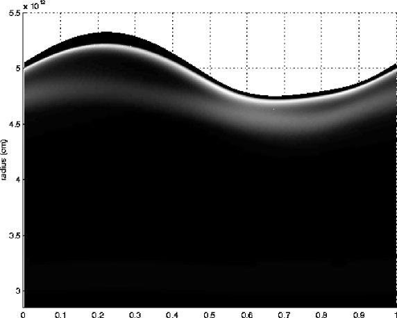
To give an indication how important time-dependence is in the pulsating Cepheid envelope we show the behavior of the turbulent energy as a function of time over a period for a typical cepheid model in Figure 1. The region of maximum turbulent energy clearly undergoes substantial motion with respect to the fluid. It also shows a widening and intensification of the turbulent region during the pulsational compression phase.

Because of this time-dependent behavior of the turbulent energy and because of the differences in the expressions for the source terms in Eqs. 2. it is of interest to see how $e_{t}$ responds in the various formulations. Gehmeyr and Winkler (1992) and Kuhfuss (1986) already compared some of the properties of their scheme to that of Stellingwerf. Here we now show some additional comparisons of the various schemes. In Figure 2 we display the temporal responses of $e_{t}$ to a constant entropy gradient $Y$ . Thus we show the results of the integration of

{d\thinspace e_{t}\over dt}={\cal C}

(15)

for two initial values of $e_{t}$ , a very small one, and a large one. The temporal response is quite different for the two values of $|N|$ , the adjustment time for $e_{t}$ to a changing source $Y$ being much slower for the larger $N$ , i.e. for the Stellingwerf choice of source. A linearization of Eq. 15 shows that the kernel has a different $e_{t}$ dependence which can lead to small differences in the spectrum of the eigenmodes.

3.2. Limit Cycles

Because the different schemes have different timescales for the turbulent energy, it is of interest to compare the nonlinear behavior of models. In Fig. 3 we show the fundamental limit cycles (light curves and radial velocity curves) for a Cepheid model with $M$ =5M_⊙, $L$ =1664L_⊙, $T_{ef\!f}$ =5400 K, $X$ =0.70, $Z$ =0.02, ( $\alpha_{d}$ = 4.0, $\alpha_{c}$ = 3.0, $\alpha_{\Lambda}$ = 0.35, $\alpha_{s}$ = 0.75, $\alpha_{\nu}$ = 1.5, $\alpha_{t}$ = 1, $\alpha_{p}$ = 0.67). Results are displayed for the three formulations $N$ =1 and $N=\pm$ 2. The calculations actually show a great insensitivity to $N$ , despite the expectations of the previous section. The reason for this insensitivity is that there are several time-scales at work, viz. a source time, a decay time and a diffusion time for $e_{t}$ . In addition, for each of the time-scales varies by many orders over the stellar envelope, as can be seen in Figure 4 which shows the run of the diffusion and of the decay time-scales for the same Cepheid model. The insensitivity is also in accord with the results of YKB who showed that a ’sudden’ approximation ( ${\cal C}=0)$ , i.e. an instantaneous adjustment of $e_{t}$ to the local static equilibrium value gives quite a good approximation to the exact linear eigenvalues.

3.3. Work Integrand

It is well known that the pulsations of the classical variable stars are self-excited through the $\kappa$ mechanism (e.g. Cox 1980, Gautschy & Saio 1995). When, for a given vibrational mode, the driving that occurs in the partial ionization regions overwhelms the damping that occurs elsewhere, the mode becomes unstable or self-excited. This can best be demonstrated by the work-integrands which show the cycle averages of $<\negthinspace pdv\negthinspace>$ throughout the star, i.e. the amount of internal energy converted into mechanical (pulsational) energy. The pressure that appears here is the total pressure $p=p_{g+r}+p_{t}+p_{\nu}$ . We can thus look at the contributions of these components separately.

In Figure 5 the total work-integrand for linear perturbations is displayed as a thick line for the fundamental Cepheid model of the previous section. Shown with arrows are the points of half-ionization of H at 11,000 K and and He^I 41,000 K, respectively. The molar tooth-shaped feature on the right is produced by the combined H and first He ionization regions which cause a broad convective region, with the spikes occurring at its boundaries. Just as in the purely radiative models the second ionization of He produces both a driving and a damping region.

The turbulent pressure plays a very small role in general, although turbulent pressure gradients can be important locally (YKB). The eddy pressure, on the contrary, is an important source of damping, especially in the limit cycle where turbulent energy is spread over a wider range. For reference, the bottom figure shows the source of turbulence, namely the dimensionless entropy gradient $Y$ , the turbulent energy, normalized to unity, and the fraction of energy carried by the convective flux $F_{c}$ . The driving is still positive in the H/He partial ionization region even though $F_{c}$ is large there. Some models, especially those with Z=0.02 can also have a convective region associated with Fe-group elements.

As is typical in the partial H/He ionization region Cepheid envelopes, convection reduces its source $Y$ by an order of magnitude, but it is not capable of reducing it at the boundaries of the convective region to less than a value of about 2–3.

3.4. Sequence of Cepheid models

In Fig. 6 we display the behavior of the relative growth-rates $\eta$ of the fundamental and first overtone modes for a sequence of Cepheid models ( $M$ =5M_⊙, $L$ =1664L_⊙, $X$ =0.70, $Z$ =0.02). The $\eta$ ’s are defined as $\eta=4\pi\kappa/\omega$ (where the linear eigenvalues are $\sigma=i\omega+\kappa$ ) and represent the pulsational energy gain per cycle (the inverse of the quality factor $Q$ in electronic circuits). (The models for the four sequences differ slightly because the small, but nonzero turbulent flux affects the equilibrium.) The four recipes are seen to give almost the same results, again showing that the time-dependence of the recipes is not critical. This is also in agreement with what YKB found, namely that the sudden approximation (instant adjustment of $e_{t}$ to the instantaneous static solution) is an excellent approximation. This is in contrast to the frequently made, but bad approximation of ’freezing’ the convective flux in the computation of the linear eigenvalues.

We conclude this section by noting that the three recipes give very similar behavior, and that the apparent differences in the published results are most likely due to different choices of the $\alpha$ parameters than to the recipes themselves.

4. Results

4.1. Light-Curve Fourier Decomposition Coefficients

In the Introduction we mentioned the presence of resonances in Cepheids between the self-excited pulsational mode and an overtone, and that this is the reason why the Fourier decomposition coefficients of the light-curves and of the radial velocity curves show so much structure in the Cepheids. RR Lyrae are devoid of such resonances and show a relatively dull behavior of the Fourier decomposition coefficients as a function of period. The presence of these resonances puts very severe constraints on Cepheid models that any turbulent convective description must satisfy (see below).

Purely radiative models were unable to reproduce the large excursion of the “Z” shape of the $\phi_{21}$ Fourier coefficient for the overtone Cepheids (e.g. Buchler 1998, Antonello & Aikawa 1993, 1995; Schaller & Buchler, 1994, unpublished preprint). It came therefore as a pleasant surprise when the nonlinear turbulent convective overtone Cepheid models showed the ability to reproduce wide excursions in the $\phi_{21}$ such as indicated by the observations. However, since extensive nonlinear calculations are needed, a systematic study of the Fourier coefficients remains to be made.

4.2. Double-Mode Pulsations in Cepheids and RR Lyrae

The numerical modelling of steady, nonlinear double mode (DM) pulsations has been a long-standing quest in which purely radiative models have failed. In a recent paper (Kolláth et al. 1998) it was found that with the inclusion of a 1D turbulent convection recipe in the code, DM pulsations appear quite naturally in Cepheid models. Almost concomitantly, but independently, Feuchtinger (1998b) encountered DM pulsations in RR Lyrae, which we have since also confirmed.

Buchler et al. (1999) show that the behavior of the double mode phenomenon both in Cepheids and in RR Lyrae can be captured by rather simple amplitude equations (also called normal forms). Here $A_{0}$ and $A_{1}$ denote the modal amplitudes of the two excited vibrational modes.

	$\displaystyle{d\thinspace A_{0}\over dt}=\bigl{(}\kappa_{0}-q_{00}A_{0}^{2}-q_{01}A_{1}^{2}\thinspace-r_{0}A_{0}^{\scriptstyle 4}\bigr{)}\thinspace\thinspace A_{0}$		(16)
	$\displaystyle{d\thinspace A_{1}\over dt}=\bigl{(}\kappa_{1}-q_{10}A_{0}^{2}-q_{11}A_{1}^{2}\thinspace-r_{1}A_{1}^{\scriptstyle 4}\bigr{)}\thinspace\thinspace A_{1}$		(17)

The transient evolution of a hydrodynamics model is governed by these equations (Kolláth et al. 1999). Furthermore, and more importantly, the fixed points of these amplitude equations ( $dA_{0}/dt=dA_{1}/dt=0$ ) allow an overview of the ’modal selection’ (bifurcation diagram) in the physical space of $L$ and $T_{ef\!f}$ , for example.

Kolláth et al. 1999 have computed double-mode pulsations with both the YKB and the GW formulations (Eqs. 2.). Both recipes give rise to DM pulsations in broad domains of the physical ( $L$ , $M$ , $T_{ef\!f}$ ) and ( $\alpha$ ) parameter space. We note that the DM behavior occurs in Galactic as well as in MC Cepheid models (Kolláth et al. 1999).

We have recently found that correcting the recipe (Eq. 2. for small Péclet number (see below) allows one to find also overtone double-mode pulsations (as are observed), in which the first and second overtones are excited.

We finish this section by stressing that the range of observed double-mode periods, amplitude ratios and Fourier phases provides a powerful set of constraints on the model parameters. This is true not only for the DM fundamental–1^st overtone and 1^st–2^nd pulsators, but also for the single mode Cepheids and RR Lyrae.

4.3. RR Lyrae pulsations

Extensive computations of convective RR Lyrae model pulsations have been made by Feuchtinger (1998a, 1999) and Feuchtinger & Dorfi (1997) using the Gehmeyr-Winkler recipe (Eqs. 2.), but omitting the turbulent flux and the turbulent pressure, and by Bono et al. (1997), using the Stellingwerf prescription. These results are reviewed by Feuchtinger in this Volume.

5. Observational Constraints

In the Introduction we have pointed out that purely radiative models have failed in many respects. In the previous section we have discussed the recent successes of the turbulent convective computations, and we have compared them to the results of the prior radiative modelling. Despite the early optimism that these successes have generated, there remain some very serious discrepancies. That they are more apparent in the Cepheid models than in RR Lyrae is not astonishing. RR Lyrae stars, despite their observed differences, are really very similar to each other in mass, luminosity and composition. The observational data of the Cepheids, on the other hand, span more than an order of magnitude in luminosity and in mass, and the metallicity of the Galactic Cepheids is four to five times that of the SMC Cepheids. These observations impose a number of important constraints that we now address.

5.1. Resonances and Mass–Luminosity relation

In 1928 Hertzsprung noticed that a bump on the light curves of the fundamental Cepheids that moved from the descending branch of the light curve to the ascending one at a pulsational period $P_{0}\sim 10$ d. Later it was found that this Hertzsprung bump progression and its corresponding manifestation in the Fourier decomposition coefficients is related to a resonance of the fundamental mode of pulsation with the second overtone (Simon & Schmidt 1976, Buchler & Goupil 1984).

It is well established by now that structure in the behavior of the Fourier decomposition coefficients of light curves and radial velocity curves as a function of, usually, the period or effective temperature, is related to resonances. Because the structure of the stellar envelope changes with this ’control’ parameter, the periods and period ratios also change and the excited pulsation mode can run into a resonance condition with an overtone which then gets entrained by this resonance through nonlinear coupling (e.g. Buchler 1993). There are two reasons for the prominence of the Hertzsprung resonance. First, the period ratio $P_{0}/P_{2}=2$ is small, making the modal coupling very low order and thus strong. Second, the second overtone, while linearly stable, is only slightly stable, which allows it to be entrained to an appreciable amplitude through the resonance.

For the first overtone Cepheids, there is also a 2:1 resonance which occurs in the lightcurve data at a period around 3–4 d (Antonello et al. 1990). More recently this resonance has also been found to be quite prominent in the radial velocity data (Kienzle et al. 1999).

The data from the microlensing surveys indicate that both these resonances occur at the same pulsation periods, to within a day. These constraints allow us to compute ’resonance’ masses and luminosities as a function of Z for stars in the instability strip. In other words it allows us to determine points on the mass-luminosity curve that these stars must obey. In a recent Letter Buchler, Kolláth, Goupil & Beaulieu (1996) discussed the implications of these resonances for Cepheid models, and they showed that there is a serious discrepancy between the pulsational models and stellar evolution calculations, with in particular the pulsation masses being much too small for the SMC models. Those results were obtained with purely radiative models.

We have since reexamined the problem with the turbulent convective models. The computed resonance luminosities still turn out largely independent of Z as suggested by the observations (Beaulieu, private communication), and the resonance masses are still much smaller for the lower Z values. One notes though that lower masses are in agreement with the evolutionary calculations (e.g. Chiosi et al 1993, Schaller et al. 1992, Baraffe et al. 1998). However, reconciling these results with reasonable widths for the instability strips remains a problem.

5.2. Largest First Overtone Period

The largest observed periods for the Galactic overtone Cepheids are $P_{1\thinspace max}=7\hbox{$.\!\!^{\rm d}$}57$ for V440 Per, $P_{1\thinspace max}=5\hbox{$.\!\!^{\rm d}$}44$ for X Lac (Antonello et al. 1990). Beaulieu quotes $P_{1\thinspace max}=5\hbox{$.\!\!^{\rm d}$}84$ for star No. 114 in the LMC, $P_{1\thinspace max}=5\hbox{$.\!\!^{\rm d}$}98$ for star No. 255 in the SMC. The star V440 may be an oddball and if we can ignore it, then there appears to be a metallicity independent upper limit $P_{1\thinspace max}\,\raise 2.0pt\hbox{$>$}\kern-8.0pt\lower 2.0pt\hbox{$\sim$}\,6$ d. The overtone periods in the beat Cepheids do not provide any upper limit here, because all of them are considerably smaller than the periods of the single-mode overtone Cepheids.

For the following discussion we refer to Fig. 12 of YKB that shows Hertzsprung -Russell diagrams with the shapes of the fundamental and first overtone instability strips (IS) for Cepheids. The overtone IS is pinched off above a certain luminosity (or period). We refer to the overtone period at the tip of the overtone IS as $P_{1\thinspace max}$ .

We can adjust the $\alpha$ parameters so that for Galactic Cepheid models (typified by X=0.70, Z=0.02) we get an upper limit of $P_{1\thinspace max}=6d$ . If, with the same $\alpha$ ’s we now compute the $P_{1\thinspace max}$ for SMC composition (typified by X=0.726, Z=0.004) we obtain values exceeding 12 d for a broad range of $\alpha$ parameters, which is clearly not in agreement with the observations. Furthermore, if we take a larger $Z$ value for the Galaxy, as is sometimes suggested, the discrepancy worsens. Conversely, adjusting the $\alpha$ ’s to get $P_{1\thinspace max}$ in agreement with the SMC value gives maximum overtone periods that are far too small for the Galaxy.

The problem arises because the lower masses and the low metallicity of the MC Cepheids. For the same luminosity and $\alpha$ ’s these stellar models are more unstable (larger $\eta$ ’s) than their Galactic siblings, which pushes the $P_{1\thinspace max}$ to much higher values. At this time a resolution of this difficulty appears to pose a serious challenge to convective Cepheid modelling.

5.3. Width of Instability Strip

Adjusting our $\alpha$ ’s so that the Galactic $P_{1\thinspace max}$ is $\sim 6\hbox{$.\!\!^{\rm d}$}0$ we invariably obtain (at the luminosity for that overtone period) a width for the fundamental IS that exceeds 1000K. We consider such a width quite excessive because in addition to the intrinsic width (for a given composition) there must be substantial widening due to metallicity dispersion.

We have found that this problem may have its origin in the formulation of the convective recipes Eqs. 2., that are all derived under the assumption of efficient convection, i.e. of large Péclet number (Pe is the ratio of radiative to convective diffusion times, thus measures the radiative damping of the convective elements). But this assumption of large Pe is not satisfied everywhere in the Cepheid envelope. In Fig. 7 we display the Péclet number throughout typical Cepheid envelopes, namely $M$ =5M_⊙, $L$ =5000L_⊙, with $T_{ef\!f}$ =4600 K (solid line) and $T_{ef\!f}$ =5300 K (dotted line). As a guide we also show the behavior of the dimensionless entropy gradient $Y$ in the upper figure. The Péclet number is very large throughout most of the combined H/He^I partial ionization region, but as the blown up bottom picture shows, the second helium ionization region lies entirely in the low Pe regime. There is also a small surface region, below T=8000 K, where Pe $<$ 1. Since the second ionization stage of helium contributes substantially to the work-integrand we expect that an improved treatment of ineffective convection has a major effect on the growth-rates.

In order to accommodate the small Pe limit CD suggest an interpolation (see also Kuhfuß 1986), which after a small manipulation can be seen to be equivalent in the GW scheme to limiting $J$ , i.e. both $F_{c}$ and ${\cal S}$ in Eqs. (2.) by a factor of the form

f_{pec}={1\over 1+\alpha_{r}P\negthinspace e^{-1}}\quad,

where the Péclet number is the ratio of convective and radiative the diffusion coefficients, Pe $=D_{c}/D_{r}$ , with

D_{r}={4\over 3}{acT^{3}\over\kappa\rho^{2}c_{p}}

and

D_{c}=\Lambda e_{t}^{\scriptscriptstyle 1/2}

The definition of Pe is somewhat arbitrary and we have introduced an additional free, order unity, parameter $\alpha_{r}$ . Both the convective flux and the source term thus become proportional to Pe when Pe is small, and scale with an additional factor of $e_{t}^{\scriptscriptstyle 1/2}$ . As a result, in the static equilibrium model (if we disregard diffusion), one obtains $e_{t}\sim Y^{2}$ , instead of $e_{t}\sim Y$ , and both $F_{c}$ and ${\cal S}$ scale with $Y^{3}$ , instead of $Y^{\scriptscriptstyle{3/2}}$ .

Referring back to Fig. 7, we note that in the higher mass Cepheid models, such as this one, a strong ( $Y$ very small) convective zone can appear in the Fe ionization region $\sim$ 200,000 K.

We have performed some preliminary calculations with the Péclet factor $f_{pec}$ . Figure 8 shows the change of some of the model properties for $M$ =5M_⊙, $L$ =3184, $X$ =0.70, $Z$ =0.02, with $\alpha_{r}$ =0, 0.1 and 0.25. ( $\alpha_{c}$ = 4.0, $\alpha_{\nu}$ = 1.0, $\alpha_{s}$ = 0.75, $\alpha_{p}$ = 0.667, $\alpha_{t}$ = 1.0, $\alpha_{d}$ = 4.0, $\alpha_{\Lambda}$ = 0.58). One sees the reduced efficiency of turbulent energy source particularly in the H/He region. This figure is somewhat misleading though. The Péclet factor decreases the turbulent energy which means that in order to satisfy the observational constraints, we have to compensate by increasing some of the $\alpha$ ’s, which is not reflected in the figure.

However, the important result is that the introduction of $f_{pec}$ has a differential effect on the stability of the fundamental and first overtone modes that goes in the direction of solving the problem of the excessive width of the fundamental instability strip. That width is most sensitive to the parameter $\alpha_{r}$ which can thus quite satisfactorily be used for adjusting the width to satisfy this observational constraint.

5.4. RR Lyrae

For RR Lyrae the ’linear’ constraints are somewhat different. Here, because globular clusters have approximately the same luminosity, we know the edges of the corresponding instability strips directly from the observed fundamental (RRab) and first overtone (RRc) periods. The observed $T_{ef\!f}$ are probably too uncertain to be directly very useful, although for specific globular clusters stars they may provide useful constraints on the temperature widths of the ISs. However, it is important to keep in mind that using the linear periods for the constraints can be misleading because a model may be inside the linear instability strip, yet the corresponding limit cycle may be unstable (e.g. Buchler & Kovács 1986). In other words, the observational instability strip is narrower than the linear instability strip, and it takes nonlinear calculations to determine the former.

A great deal of observational lightcurve data are available, and their Fourier decomposition coefficients provide strong nonlinear constraints that need to be satisfied by the models. In particular there is a nice correlation between the coefficients that has been discussed by Kovács and Kanbur (1997).

The double-mode, RRd stars also provide tight constraints on the alpha parameters through the observed periods and period ratios, and through the amplitude ratios.

5.5. Additional Constraints

From the observational data one can infer period – radius relations for Cepheids (e.g. Laney & Stobie 1994). These constraints are very basic since they concern the equilibrium models. Bono et al. (1998, 1999) have had mixed success reproducing this observational constraint.

Other nonlinear interesting constraints arise from the temperature fluctuations of the Cepheids and RR Lyrae. Simon, Kanbur & Mihalas (1993) have shown that essentially all Cepheids have the same $T_{max}$ (same spectral type), but that $T_{min}$ depends on the amplitude of pulsation. Similarly, but oppositely, RR Lyrae have essentially the same $T_{min}$ (e.g. Kanbur & Phillips 1996). These constraints have not yet been taken into account in the calibration of the $\alpha$ parameters.

6. Theoretical Difficulties

For a given set of $\alpha$ s the 1D recipes all give the same turbulent energy $e_{t}$ in the equilibrium models when the turbulent flux is neglected, which is

e_{t}=\alpha_{s}^{2}\thinspace\alpha_{\Lambda}^{2}\thinspace{\beta T\over\Gamma_{1}}\thinspace c_{s}^{2}\thinspace Y{\rm\quad or\quad}u_{t}\sim c_{s}\sqrt{Y}

(18)

When this $e_{t}$ is inserted in the expression for convective flux one obtains

F_{c}=\alpha_{c}\alpha_{\Lambda}\thinspace(\rho c_{p}T)\thinspace c_{s}Y^{\scriptstyle{3/2}}

(19)

However, $F_{c}$ is physically limited to transporting the available energy fluctuations whose very generous upper limit is $(\rho c_{p}T)$ . Furthermore, under the underlying assumptions the convective velocity should be subsonic. Eq. (19) clearly exceeds this upper limit when $Y$ is larger that unity (cf. Fig. 7). For this reason ad hoc flux limiters have been proposed (e.g. Feuchtinger 1999)

The ultimate reason for the breakdown of the 1D recipe is twofold. First, in the convective boundary regions where $Y\,\raise 2.0pt\hbox{$>$}\kern-8.0pt\lower 2.0pt\hbox{$\sim$}\,1$ , the turbulent Mach number $M_{t}=(u_{t}/c_{s})$ invariably becomes important and can even exceed unity in some weakly convective models. However, it is well known that the approximations leading to the recipes Eqs. (2.) break down, in particular because pressure fluctuations were neglected in their derivations and the dissipation term $\epsilon$ does not take into account larger Mach numbers. Second, as stressed by Canuto (1998) the downgradient approximations for the fluxes (here $F_{c}\sim ds/dr$ ) are not very satisfactory. Neither of these problems can easily be corrected within a practically useful 1D recipe, and a flux limiter may be the most expedient available patch.

7. Conclusions

The introduction of a simple recipe for turbulent convection, namely a 1D time-dependent diffusion equation for the turbulent energy and the concomitant expressions for convective and turbulent fluxes, eddy viscous pressure and turbulent pressure, have provided a substantial improvement over purely radiative models. Perhaps the most remarkable achievement is the successful modelling of double-mode pulsations both in Cepheids and in RR Lyrae. Correcting the recipes for low Péclet number provides a further definite improvement.

However, a number of problems persist as we have seen. The number (8) of free, order unity parameters is large which makes a search for optimal values quite burdensome. We still hope that it will be possible to find a range of suitable parameters that satisfy all the observational constraints, and this independently of metallicity or of the stellar type. If not we will be forced to adopt more complicated formulations of convective transport.

Acknowledgments.

We are much obliged to Phil Yecko and Michael Feuchtinger for many discussions. Phil kindly provided us with Figure 1. We also wish to thank Vittorio Canuto for fruitful conversations and for suggesting the use of his formalism to discriminate among the various one-equation approximations. Finally, we gratefully acknowledge the support of NSF (AST95–28338) and ZK the support of OTKA (T-026031).

References

Antonello, E. & T. Aikawa, 1993 AA 279, 119; 1995 AA 302, 105

Antonello, E., Poretti, E. Reduzzi, L, 1990, AA 180, 129

Baraffe, I., Y. Alibert, D. M’era, G. Chabrier, & J. P. Beaulieu, 1998, ApJ Lett. 499, 205

Bono, G., F. Caputo, V. Castellani & M. Marconi, 1997, AA 121, 327.

Bono, G., F. Caputo, & M. Marconi, 1998, ApJLett 497, L43

Bono, G., F. Caputo, V. Castellani, & M. Marconi, 1999, ApJ 512, 711

Bono, G. & R. F. Stellingwerf, 1994, ApJ Suppl 93, 233–269

Buchler, J.R. 1993, in Nonlinear Phenomena in Stellar Variability, Eds. M. Takeuti & J.R. Buchler, Dordrecht: Kluwer Publishers, reprinted from 1993, Ap&SS, 210, 1–31.

Buchler, J. R. 1998, in A Half Century of Stellar Pulsation Interpretations: A Tribute to Arthur N. Cox, eds. P.A. Bradley &J.A. Guzik, ASP 135, 220

Buchler, J. R., P. Yecko, Z. Kolláth & M. J. Goupil, 1999, Turbulent Convection in Pulsating Stars, in Theory and Tests of Convection in Stellar Structure, ASP Conference Series, Vol 173, 1999, A. Gimenez, E.F. Guinan and B. Montesinos, Eds.

Buchler, J. R. & M. J. Goupil, 1984, ApJ 279, 394

Buchler, J.R., Z. Kolláth, J. P. Beaulieu,, M. J. Goupil, 1996, ApJLett 462, L83

Buchler, J.R. & Z. Kovács, 1986, ApJ 308, 661

Canuto, V. M. & M. Dubikov, 1998, ApJ 493, 834

Canuto, V.M. 1998, ApJ 508, 767

Chiosi, C., P. Wood & N. Capitanio 1993, ApJS 86, 541

Cox, A. N. 1980, Ann. Rev. Astr. Astrophys., 18, 15

Ferlet, R., J. P. Maillard, & B. Raban, 1996, Variable Stars and the Astrophysical Returns of Microlensing Surveys, Proceedings of the Twelfth IAP Colloquium, Editions Frontières

Feuchtinger, M. U. 1998a, AA Suppl 136, 217

Feuchtinger, M. U. 1998b, AA 337, L29

Feuchtinger, M. U. & E. A. Dorfi, 1997, AA 322, 817

Feuchtinger, M. U. 1999, AA (in press)

Gautschy, A. & H. Saio, 1995, Ann. Rev. Astr. Astrophys 33, 75 and 1996, ibid. 34, 551

Gehmeyr, M. 1992, ApJ 399, 265

Gehmeyr, M. & K.-H. Winkler, 1992, AA 253, 92 ; ibid. 253, 101

Kanbur, S. & P. M. Phillips, 1996, AA 314, 514

Kienzle, F., P. A. Moskalik, D. Bersier, & F. Pont, 1999, AA 341, 818-826

Kolláth, Z., J.P. Beaulieu, J. R. Buchler, & P. Yecko, 1998, ApJ Lett 502, L55

Kolláth, Z., J. R. Buchler, P. Yecko, R. Szabó, & Z. Csubry, 1999 (in preparation)

Kovács, G. & S. Kanbur,1997, MNRAS 295, 834.

Kuhfuß, R. 1986, AA 160, 116

Laney, C. D. & R. S. Stobie, 1994, MNRAS 266, 441

Moskalik, P., J. R. Buchler, & A. Marom, 1992, ApJ 385, 685–693

Rieutord, M. & J.-P. Zahn, 1995, AA 296, 127

Schaller G., D. Schaerer, G. Meynet & A. Maeder, 1992, AA 96, 269

Simon, N. R. & E. G. Schmidt, 1976, ApJ 205, 162

Simon, N. R., S. Kanbur, & D. Mihalas, 1993, ApJ 414, 310

Stellingwerf, R.F. 1982, ApJ 262, 330

Yecko, P., Z. Kolláth, J. R. Buchler, 1998, AA 336, 553 [YKB]