PSCz-1.2 Jy Comparison: A Spherical Harmonics Approach

Abstract

We perform a detailed comparison of the IRAS PSCz and 1.2-Jy spherical harmonic coefficients of the density and velocity fields in redshift space. The monopole terms predicted from the two surveys show some differences. The mismatch between the velocity monopoles arises from faint sources and disappears when extracting a PSCz subsample of galaxies with fluxes larger than 1.2 Jy. The analysis of PSCz dipole moments confirms the same inconsistencies found by Davis, Nusser and Willick (1996) between the IRAS 1.2-Jy gravity field and MARK III peculiar velocities. We conclude that shot-noise, which is greatly reduced in our PSCz gravity field, cannot be responsible for the observed mismatch.

1 Introduction

Nusser & Davis (1994) show that in linear gravitational instability (GI) theory the peculiar velocity field in redshift space is irrotational and thus can be expressed in terms of a potential: ${\vec{v}}=-\nabla\Phi(\vec{s})$. The angular dependencies of the potential velocity field and the galaxy overdensity field [both measured in redshift space and expanded in spherical harmonics, $\Phi_{lm}(s)$ and $\hat{\delta}_{lm}(s)$, respectively] are related by a modified Poisson equation:

$${{1}\over{s^{2}}}{{d}\over{ds}}\left(s^{2}{{d\Phi_{lm}}\over{ds}}\right)-{{1}\over{1+\beta}}{{l(l+1)\Phi_{lm}}\over{s^{2}}}={{\beta}\over{1+\beta}}\left(\hat{\delta}_{lm}-{{1}\over{s}}{{d\ln{\phi}}\over{d\ln{s}}}{{d\Phi_{lm}}\over{ds}}\right),$$ (1)

where $\phi(s)$ is the selection function. To solve this differential equation we first compute the density field on an angular grid using cells of equal solid angle and 52 bins in redshift out to $s=18\,000$ kms^-1.

$$1+{\hat{\delta}}_{j}({\vec{s}}_{n})=\frac{1}{(2\pi)^{3/2}\sigma_{1.2n}^{3}}\sum_{i}^{N_{j}}\frac{1}{\phi(s_{i})}\exp\left[-\frac{({\vec{s}}_{n}-{\vec{s}}_{i})^{2}}{2\sigma_{1.2n}^{2}}\right]$$ (2)

where the sum is over all the galaxies within the catalogue $j$, $N_{j}$. The Gaussian smoothing width for the cell $n$ at redshift $s_{n}$, $\sigma_{1.2n}$, is given by $\sigma_{1.2n}=[\bar{n}_{1.2}\phi_{1.2}(s_{n})]^{-1/3}$ (or 100 km s${}^{-1}~{}$when such a length is smaller than this), where $\bar{n}_{1.2}$ and $\phi_{1.2}$ are the 1.2 Jy mean number density and selection function, respectively.

2 Datasets

PSCz is a new redshift survey which resulted from a collaborative effort involving several British institutions (Durham, Oxford, London, Edinburgh and Cambridge). The catalogue contains some 15500 IRAS PSC (Point Source Catalogue) galaxies with a 60 $\mu$m flux larger than 0.6-Jy. This survey covers 84$\%$ of the sky. A more detailed description of the catalogue is given by Saunders et al. 1999 (these proceedings). The 1.2-Jy catalogue (Fisher et al. 1995) contains 5321 IRAS PSC galaxies with a 60 $\mu m$ limit of 1.2-Jy which covers 87.6$\%$ of the sky.

3 Results, Discussion and Conclusions

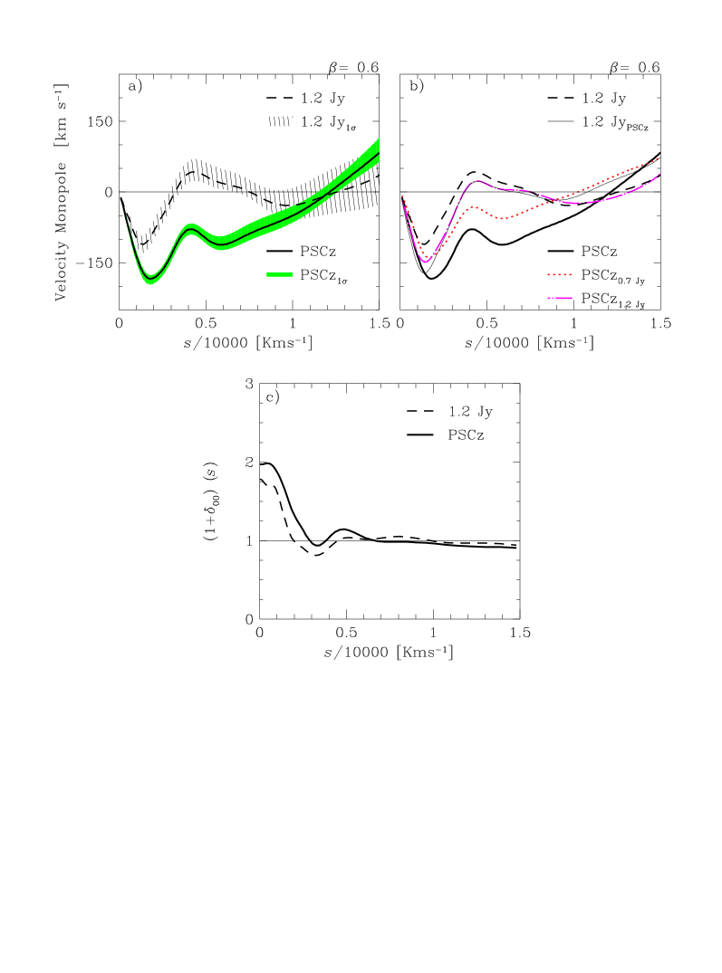
Figure 1: Monopole coefficients, $u_{00}(s)$ and ${\hat{\delta}}_{00}(s)$, estimated from PSCz and 1.2-Jy catalogues for $\beta=0.6$. On the two top panels dashed (thick) lines represent 1.2-Jy (PSCz) monopole mode of the velocity field. a) The hatched and shaded regions indicate the 1.2 Jy and PSCz 1–$\sigma$ shot-noise uncertainties, respectively. b) Dotted, dot-dashed and thin lines represent PSCz_0.7, PSCz_1.2 and 1.2-Jy${}_{\mbox{PSCz}}$, respectively. c) The thick line indicates the PSCz density monopole while the 1.2-Jy counterpart is represented by the dashed line.

We compare the line of sight peculiar velocity, $u({\vec{s}})\equiv[{\vec{v}}({\vec{v}})-{\vec{v}}_{LG}]\cdot{\hat{s}}$, and density perturbations, $\hat{\delta}(s)$, fields inferred from the IRAS PSCz and 1.2-Jy redshift surveys, in redshift-space. To compute the spherical harmonics coefficients up to $l_{max}=16$ we apply the algorithm introduced by Nusser & Davis (1994) setting $\beta=0.6$.

In Fig. 1 we display the monopole of the velocity field, $u_{00}$ (two top panels) and the monopole of the density ${\hat{\delta}}_{00}$ (bottom panel). In the top-left panel, the estimate of the velocity monopole in the 1.2-Jy (dashed line) is systematically larger than the PSCz one (continuous thick line) within a redshift of $s\approx 8000$ km s^-1. The density monopole of the two surveys show a similar qualitative radial dependency (bottom panel). In Fig. 2 we show the three velocity dipole terms of the two surveys along with the total amplitude (bottom left panel). The various dipole moments exhibit good agreement, except $u_{11}$ (top left panel) for which there is a discrepancy of 100 km$s^{-1}$ in the redshift range $1500-7500$ kms^-1. Good agreement is also found when comparing higher order multipoles (Teodoro et al. 1999). Note that when all the multipoles are considered (i.e. when performing a full v-v comparison) the PSCz and 1.2-Jy gravity fields look fully consistent (Branchini et al. 1999).

In all plots, shaded and hatched regions represent 1-$\sigma$ shot-noise uncertainties computed from 20 bootstrap realizations of PSCz and 1.2 Jy surveys, respectively. Where does the discrepancy between the monopoles of the PSCz and 1.2 Jy surveys come from? As shown in the plots, the difference is larger than that expected from the shot-noise. Tadros et al. (1999) have suggested that the PSCz catalogue may be incomplete for fluxes $\leq 0.7$ Jy. If true, then we would expect that the velocity monopole for the PSCz with a flux cut at 0.7 Jy (PSCz_0.7) would be in good agreement with the 1.2-Jy survey. The dotted line ($u_{00,\mbox{PSCz}_{0.7}}$) in the top panel of Fig. 1 shows however that this is not case. It is only in cutting the PSCz catalogue at a flux level of 1.2 Jy that, as expected, the discrepancy disappears, provided that we use the same mask for both catalogues. This is clearly seen in the top right panel of Fig. 1 in which the thin and dot-dashed lines indicate 1.2-Jy_PSCz(1.2 Jy with the same mask as PSCz) and PSCz_1.2-Jy (PSCz with a 1.2 Jy flux limit) velocity monopoles, respectively.

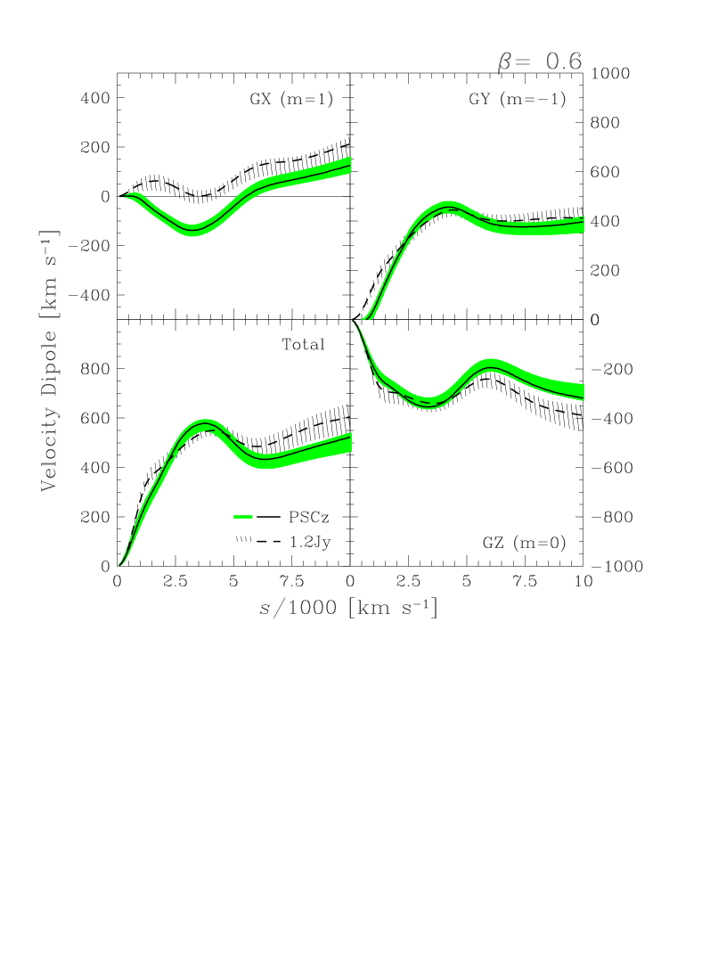
Figure 2: The dipole coefficients, $u_{1m}(s)${$m=-1,0,1$}, inferred from PSCz and 1.2-Jy for $\beta=0.6$. The solid and dashed lines in the various panels represent PSCz and 1.2-Jy dipoles, respectively. The $GX$, $GY$, $GZ$ panels show the three Galactic components of the dipole and the bottom left is their quadrature sum. Hatched and shaded regions indicate the 1.2-Jy and PSCz 1–$\sigma$ shot-noise uncertainty, respectively.

A more detailed comparison between the two catalogues is in progress in which we assess the importance of systematic errors by using a suite of 1.2 JY and PSCz mock catalogues drawn from N-body simulations.